HAL Id: halshs-00492204
https://halshs.archives-ouvertes.fr/halshs-00492204
Submitted on 15 Jun 2010
HAL is a multi-disciplinary open access
archive for the deposit and dissemination of sci-entific research documents, whether they are pub-lished or not. The documents may come from teaching and research institutions in France or abroad, or from public or private research centers.
L’archive ouverte pluridisciplinaire HAL, est destinée au dépôt et à la diffusion de documents scientifiques de niveau recherche, publiés ou non, émanant des établissements d’enseignement et de recherche français ou étrangers, des laboratoires publics ou privés.
Markups and the Welfare Cost of Business Cycles : A
Reappraisal
Jean-Olivier Hairault, François Langot
To cite this version:
Jean-Olivier Hairault, François Langot. Markups and the Welfare Cost of Business Cycles : A Reap-praisal. 2010. �halshs-00492204�
Documents de Travail du
Centre d’Economie de la Sorbonne
Markups and the Welfare Cost of Business Cycles :
A Reappraisal
Jean-Olivier H
AIRAULT,François L
ANGOTMarkups and the Welfare Cost of Business Cycles: A Reappraisal
Jean-Olivier Hairault
Paris School of Economics (PSE) & University Paris 1 & IZA
joh@univ-paris1.fr
Franc¸ois Langot
GAINS-TEPP (U. du Mans) & Cepremap & IZA
flangot@univ-lemans.fr March 2010
Abstract
Gali et al. (2007) have recently shown in a quantitative way that inefficient fluctuations in the allocation of resources do not generate sizable welfare costs. In this note, we show that their evaluation underestimates the welfare costs of inefficient fluctuations and propose a biased estimate of the impact of structural distortions on business cycle costs. As monop-olistic suppliers, both firms and households aim at preserving their expected markups; the interaction between aggregate fluctuations in the efficiency gap and price-setting behaviors results in making average consumption and employment lower than their counterparts in the flexible price economy. This level effect increases the welfare cost of business cycles. It is all the more sizable in that the degree of inefficiency is structurally high at the steady state.
Keywords: Business cycle costs, inefficiency gap, new-Keynesian macroeconomics
1
Introduction
New-Keynesian Macroeconomics (Mankiw (1985), Ball and Romer (1989), Gali et al. (2007)) often claims that there are potentially large business cycle costs due to the asymmetrical effect on welfare of expansions and recessions. There is indeed a fundamental asymmetry, provided that the deterministic monopolistic economy is far from the first best allocation: expansions are improving as they bring the economy closer to the social optimum; recessions are welfare-degrading as they push the economy further from the social optimum. Does this imply that business cycles are costly on average, in the traditional sense that the economy with fluctuations (the stochastic economy) is welfare-dominated by the (same) economy without fluctuations (the deterministic economy)? Gali et al. (2007) show in a quantitative way that inefficient fluctuations in the allocation of resources do not generate sizable welfare costs, although the recessions do indeed reduce welfare more than expansions increase it. In this note, we show that their evaluation underestimates the welfare costs of inefficient fluctuations and propose a biased estimate of the impact of structural distortions on business cycle costs.
As Gali et al. (2007) aim at measuring business cycle costs in a realistic economy, they consider a relatively highly distorted economy. In that case, the welfare cost of the volatility in the efficiency gap is low: the more distorted the deterministic economy, the lower the business cycle costs due to the volatility in the efficiency gap (volatility effect) as welfare gains from expansions almost compensate for welfare losses from recessions. However, once sizable structural distortions are considered at the steady state, and this is essential for the Keynesian argument of asymmetry between recessions and expansions, it is no longer relevant to neglect the effect of volatility on mean aggregates in welfare computations (Sutherland (2002), Woodford (2003), Benigno and Woodford (2005) and Gali (2008)). Quite surprisingly, Gali et al. (2007) leave aside this potential source of business cycle costs (level effect). Optimal monetary policy in the case of a distorted steady state has been already scrutinized by Benigno and Woodford (2005). They show that a linear-quadratic approximation to the optimal policy problem is still valid in the case of a distorted steady state. By taking into account the effects of the business cycle and of the stabilization policy on the average aggregates, they also emphasize that the degree of the structural inefficiency affects the weights on inflation and the output gap in the objective function of the central bank. However, they do not propose an analysis of the relative importance of the level effect to the welfare costs of business cycles. This paper fills this gap in a simplified theoretical framework which allows us to uncover some basic properties of a distorted steady state new-Keynesian economy in the business cycles along the lines of Gali et al. (2007). Our contribution is to show in a simple new-Keynesian framework with pre-determined prices `a
la Ball and Romer (1987) that the level effect may dominate the volatility effect and make the
(total) business cycle costs increase with the degree of the structural distortions. As monopolistic suppliers, both firms and households aim at preserving their expected markups; the interaction
between aggregate fluctuations in the efficiency gap and price-setting behaviors results in mak-ing average consumption and employment lower than their counterparts in the flexible price economy. This level effect increases the welfare cost of business cycles. It is all the more sizable in that the degree of inefficiency is structurally high. In a nutshell, there are potentially more business cycle costs than usually considered and a more distorted economy can generate higher business cycle shocks. Quite interestingly, this is all the more true if the economy displays Keynesian features, i.e. the labor supply elasticity is weak and demand shocks contribute more than technological shocks to the inefficiency gap volatility. Finally, our analysis provides some quantitative arguments for considering the case of a distorted steady state in any monetary policy analysis.
The next section presents a canonical new-Keynesian model with preset prices and wages. Sec-tion 3 derives its implicaSec-tions for the expected inefficiency gap and the mean aggregates relative to the flexible-price economy. Section 4 computes the welfare cost of business cycles in a highly distorted economy. Section 5 concludes.
2
A canonical NKM framework
We consider a one-period economy along the lines of Ball and Romer (1989). This simple model is consistent with the reduced-form model proposed by Gali et al. (2007) and will allow us to easily derive our main results.
Preferences. For an individual j, we assume that the preferences can be summarized by the following utility function:
Uj = µ ν − 1 ν ¶ Cj,t1−σ 1 − σ− µ ε − 1 ε ¶ Nj,t1+φ 1 + φ where Cj = µZ 1 0 Cε−1ε j,i di ¶ ε ε−1
σ is the coefficient of relative risk aversion and φ measures the extent of increasing marginal
disutility of labor. The coefficient on consumption and labor are chosen for convenience. ε is the elasticity of substitution between any two goods (ε > 1). The demand for any good i is given by: Cj,i= µ Pi P ¶−ε Cj ∀i
Technology. We assume that technology is linear with only labor input: Y = AN . A tech-nological shock A hits the production function at each time with E[A] = 1. Due to imperfect
substitutability between goods, the competition between firms is monopolistic. The labor used to produce each good is a CES aggregate of the continuum of individual types of labor:
N = µZ 1 0 Nν−1ν j dj ¶ ν ν−1
ν is the elasticity of substitution between any two skills (ν > 1). Due to imperfect substitutability
between skills, the competition between individuals is monopolistic. We can derive the demand for any skill j as follows:
Nj = µ Wj W ¶−ν N ∀j
Money Demand. We assume that money is required for transactions: C = M/P .
Preset prices and wages. Prices and wages are set before the money supply and technology are known. Let us turn to the monopolistic firm i which faces a general price index P0, an
aggregate wage index W0, a demand function Ci = ³
Pi
P0
´−ε
C. At the symmetric equilibrium,
the optimal price satisfies:
E · ε − 1 ε − w0 M P N ¸ = 0 (1)
where w0= WP00 and M P N denotes the marginal product of labor.
Let us turn now to the monopolistic individual j who faces P0, W0 and a demand function
Nj =
³
Wj
W0
´−ν
N . At the symmetric equilibrium, the optimal wage satisfies: E · ν − 1 ν − M RS w0 ¸ = 0 (2)
where M RS denotes the marginal rate of substitution between consumption and leisure.
Market Equilibrium. At general equilibrium, we have C = M/P = Y = AN .
3
Expected efficiency gap and average aggregates
In this section, it is shown that the price-setting behavior in a monopolistic environment leads consumption, employment and output to be inferior on average to their deterministic counter-parts.
Let us define the efficiency gap along the lines of Gali et al. (2007):
GAP = M RS M P N
where GAP ∈ [0; 1]. Without aggregate fluctuations or in a flexible-price economy, the value of the efficiency gap is constant and equal to ¡ε−1
ε
¢ ¡ν−1
ν
¢
≡ GAP . Let us define Φ a measure of
the structural inefficiency due to monopolistic competition on both labor and good markets: 1 − Φ = µ ε − 1 ε ¶ µ ν − 1 ν 
On the other hand, when there are price and wage rigidities in a stochastic environment, the efficiency gap depends on the realization of the shocks according to the following equation:
GAP = (1 − Φ) µ M P0 ¶σ+φ A−(1+φ) (3)
The productivity and monetary shocks move the efficiency gap away from its deterministic value 1 − Φ. The agents preset prices and wages in a stochastic environment (Equations (1) and (2)) such that the expected efficiency gap is the solution to:
E[GAP ] = (1 − Φ) + cov(A × GAP, 1
A) (4)
Note that the average gap is equal to its deterministic counterpart only when there are monetary shocks. Even in this case, it does not imply that the average aggregates coincide with their deterministic counterparts. Equations (3) and (4) imply that P0 is preset at a value which makes the average efficiency gap consistent with its desired value. Considering the non-linearity embodied in Equation (3), it is straightforward that P0 must be set at a value different from
its deterministic counterpart. This ensures that the efficiency gap is equal to its desired value on average. In turn, average consumption and employment will differ from their deterministic counterpart. This level effect is really specific to the rigid price economy as it arises from the interaction between the fluctuations in the efficiency gap and the price-setting behavior. It leads to the average consumption and employment differing from their counterparts in the flexible price economy1.
It is possible to show more explicitly these effects by considering a second-order approximation of Equation (3) around the flexible-price path:
[
GAP ≈ (σ + φ) eC +1
2(σ + φ)
2Ce2 (5)
where the tilde denotes the log deviation from the flexible-price economy ( eC = log(C/Cf))
and the hat the relative deviation from the deterministic path ( [GAP = GAP −GAPGAP ), as in Gali et al. (2007). Note that the inefficiency gap remains constant at its deterministic value in the flexible-price economy.
1Note that the mean of the consumption can be affected even in the case where consumption does not fluctuate
in the business cycle. When there are only productivity shocks, consumption does not fluctuate as real balances are constant. However, the average consumption will be affected by the desire of the agents to satisfy condition (4).
Given that E( [GAP ) = φV ( bA) (Equation (4)), it is possible to derive the expected value of the
log-deviation of consumption from its flexible-price counterpart2:
E[ eC] = −1 2 1 σ + φ µ 1 − 2φva (1 + φ)2 ¶ var( [GAP ) (6)
with va the contribution of the technological shock to the gap volatility3.
4
The welfare cost of inefficient fluctuations
A welfare-based measurement. Let us consider a second order approximation of the welfare around the flexible price economy path as in Gali et al. (2007):
∆ = U (Ct, Nt) − U (Ctf, Ntf) ≈ Φ ˜C −
1
2[(φ + σ) − Φ(1 + φ)] ˜C
2
As is usual in the literature, we express the average welfare costs of the business cycles as follows:
E ∆ U0 Cf,tC f t ≈ ΦE( ˜C) | {z } Level Effect −1 2[(φ + σ) − Φ(1 + φ)]var( eC) | {z } Volatility Effect
The business cycle cost can be broken down into two terms. Firstly, there is a cost due to the impact of consumption volatility (var( eC)) on welfare (the volatility effect). Secondly, the
average consumption in the fluctuating economy is weaker than its flexible-price counterpart (level effect).
Volatility Effect. Let us first examine the business cycle cost due to the volatility effect. This effect is the cost that Gali et al. (2007) took into consideration. In order to measure only the inefficiency component of the consumption volatility, they substitute the inefficiency gap volatility for the consumption volatility. Using Equation (5), we have:
volatility effect = −1 2 1 σ + φ µ 1 −Φ(1 + φ) σ + φ ¶ var( [GAP )
The volatility effect comes from the asymmetry between expansions and recessions. Recessions increase the efficiency gap more than expansions decrease it. When Φ tends to zero (the deter-ministic economy is “almost” Walrasian), the impact of the volatility on the measurement of the welfare cost of business cycles increases, as even the expansions are costly, since they move the economy away from the first-best allocation. The parameters σ and φ have an ambiguous effect; for a given volatility, they decrease the business cycle costs; however, they increase the inefficiency gap volatility. The latter effect dominates and then explains why Gali et al. (2007) show that the volatility effect increases with σ and φ.
2It is possible to show that 1
P0 ≈ 1 − 1 2(σ + φ − 1)var( cM ) − 1 2 ³ 2+φ(1+φ) σ+φ ´
var( bA). If we abstract from the
technological shock (var( bA) = 0), this result is the same as in Ball and Romer (1989).
Level effect. Let us now turn to the second source of the business cycle costs. There is a loss in average consumption relative to the flexible-price economy (Equation (6)) due to the interaction between fluctuations and nominal rigidities. This loss is particularly welfare-decreasing when the structural inefficiency Φ is large, i.e. when the deterministic level of consumption is low (the marginal utility of consumption is then high). Again, it is possible to evaluate this cost in terms of the volatility in the efficiency gap. Using the equation (6), we have:
level effect = −Φ 2 1 σ + φ µ 1 − 2φva (1 + φ)2 ¶ var( [GAP )
For a given variance of the efficiency gap, the business cycle cost is increasing with the degree of distortions Φ. The lower the contribution of the technological shocks to the efficiency gap volatility, the greater the level effect for the business cycle costs. An increase in σ and φ has the same ambiguous effect: it induces higher volatility in the efficiency gap but a lower cost for any given volatility.
The relative contribution of the level effect. Traditionally, only the volatility effect is considered in the evaluation of business cycle costs. It is possible to evaluate the relative con-tribution of the level effect to the business cycle costs from the following equation:
E µ ∆ U0 CC ¶ ≈ −Φ 2 1 σ + φ µ 1 − 2φva (1 + φ)2 ¶ var( [GAP ) −1 2 1 σ + φ µ 1 −Φ(1 + φ) σ + φ ¶ var( [GAP )
The level effect accounts for a proportion γ of the business cycle costs generated by the volatility effect: γ = Φ ³ 1 − 2φva (1+φ)2 ´ 1 −Φ(1+φ)(σ+φ)
The proportion γ is increasing with Φ as the structural inefficiency gap increases the level effect and dampens the volatility effect. It is worth emphasizing that an increase in the degree of distortion at the deterministic equilibrium now has an indeterminate impact on the business cycle costs. Without taking into account the level effect, this effect is always negative: considering Φ = 0 maximizes the welfare cost of volatility. Accounting for the level effect implies that a more highly distorted economy increases the business cycle costs, provided that the productivity shock does not contribute too much to the efficiency gap volatility:
∂E ³ ∆ U0 CC ´ ∂Φ < 0 ⇔ va< (1 + φ)2(σ − 1) 2φ(σ + φ) (7)
Under the condition (7), the more distorted the economy, the higher the business cycle costs. Monopolistic competition and price rigidity may interact to magnify the costs of business cycles4. 4Let us emphasize that for σ ≥ 2.5, the condition (7) is no longer stringent. When σ = 2, the technological
On the other hand, the lower the contribution va of the technological shocks to the inefficiency
gap volatility, the higher the proportion γ. This proportion is also increasing (decreasing) with
φ (σ), despite their respective effects on the contribution of the technological shocks. Overall,
the level effect contribution can easily dominate the volatility effect, ie. γ > 1. Let us notice that for σ close to 1 and va close to 0, γ ≈ Φ/(1 − Φ). In the benchmark calibration proposed
by Gali et al. (2007) with Φ = 0.5, the level effect accounts as much as the volatility effect for the business cycle costs. For Φ = 0.65, , which is still a realistic value, γ is almost equal to 2.
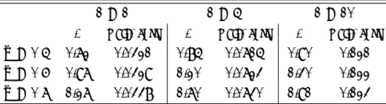
Table 1: Sensitivity Analysis
φ = 1 φ = 5 φ = 10
γ welf. cost γ welf. cost γ welf. cost
Φ = 0.5 0.72 0.0321 0.85 0.0715 0.90 0.121
Φ = 0.6 0.97 0.0329 1.20 0.0723 1.30 0.122
Φ = 0.7 1.27 0.0338 1.70 0.0730 1.91 0.123
Note: Welfare costs are expressed in percentages of permanent consumption.
It is worth emphasizing that a high contribution of the level effect does not imply that the business cycle costs are particularly small. For instance, in Table 1, considering lower values for the labor supply elasticity (higher values of φ) increases both the contribution of the level effect and the costs of business cycles5. Whereas the relative contribution of the level effect and
the total business cycle costs are equal to 0.72 and 0.03% respectively for φ = 1, both jump to 0.90 and 0.12% for φ = 10 when considering Φ = 0.5. Increasing the value of Φ has the same doubly positive influence. However, the total business cycle costs are quite insensitive to Φ. Considering a typically Keynesian economy, with both a low labor supply elasticity and a high degree of structural inefficiency, makes the level effect dominant and the business cycle costs quite sizable. When Φ reaches 0.70, the level effect accounts for almost two-third of the 0.12% permanent consumption loss.
5
Conclusion
In this paper, it is shown that the business cycle costs intrinsically implied by the price rigidity may be higher than previously shown by Gali et al. (2007). Price-setting behaviors lead to decreasing the average value of consumption and labor, relative to their flexible-price counter-parts. This level effect makes a distorted steady state economy more vulnerable to business more than three-fourths.
5For this sensitivity analysis, we consider σ = 2. We calibrate the variance of the monetary and the
techno-logical shocks such that we are able to replicate the benchmark business cycle costs in Gali et al. (2007) when we only take into account the volatility effect. We impose in this benchmark case that the technological shock contribution amounts to 10% of the inefficiency gap volatility.
cycles, contrary to the traditional volatility effect.
On the other hand, when considering optimal policies it is traditionally assumed that the struc-tural distortions are totally eliminated by appropriate subsidies. In this case, it is consistent to put aside the level effect as its implied cost is nil. However, as recently emphasized by Benigno and Woodford (2005), Khan et al. (2003) and Schmitt-Groh´e and Uribe (2007), this case is quite artificial and optimal monetary policy deserves to be analyzed in a distorted steady state economy. Our paper shows that considering a distorted economy can worsen the consequences of aggregate fluctuations for the output gap. The next question is to investigate the optimal monetary policy in this context. Although Benigno and Woodford (2005) have already shown that the basic principles of monetary policy can be saved, how aggressively the central bank should react to the output gap could be changed when the level effect is accounted for. This point is left for future research.
References
Ball, L. and D. Romer (1989), ‘Are prices too sticky?’, Quarterly Journal of Economics 104, 507– 24.
Benigno, P. and M. Woodford (2005), ‘Inflation stabilization and welfare: The case of a distorted steady state’, Journal of the European Economic Association 3, 1–52.
Gali, J. (2008), Monetary Policy, Inflation and the Business Cycle: An Introduction to the New
Keynesian Framework, Princeton University Press.
Gali, J., M. Gertler and D. Lopez-Salido (2007), ‘Markups, gaps, and the welfare costs of business fluctuations’, The Review of Economics and Statistics 89, 44–59.
Khan, A., King R. and A. Wolman (2003), ‘Optimal monetary policy’, Review of Economic
Studies 70, 825–860.
Mankiw, G. (1985), ‘Small menu costs and large business cycles’, Quarterly Journal of Economics 100, 529–37.
Schmitt-Groh´e, S. and M. Uribe (2007), ‘Optimal, simple, and implementable monetary and fiscal rules’, Journal of Monetary Economics 54, 1702–1725.
Sutherland, A. (2002), A simple second-order solution method for dynamic general equilibrium models. CEPR discussion paper no. 3554, July.
Woodford, M. (2003), Interest and Prices: Foundations of a Theory of Monetary Policy, Prince-ton University Press.
![[PDF] Langage Python cours de base avec exemples | Formation informatique](data:image/gif;base64,R0lGODlhAQABAIAAAP///wAAACH5BAEAAAAALAAAAAABAAEAAAICRAEAOw==)