Cross-validation failure: small sample sizes lead to large error bars

HAL Id: hal-01545002

https://hal.inria.fr/hal-01545002

Submitted on 22 Jun 2017

HAL is a multi-disciplinary open access

archive for the deposit and dissemination of

sci-entific research documents, whether they are

pub-lished or not. The documents may come from

teaching and research institutions in France or

abroad, or from public or private research centers.

L’archive ouverte pluridisciplinaire HAL, est

destinée au dépôt et à la diffusion de documents

scientifiques de niveau recherche, publiés ou non,

émanant des établissements d’enseignement et de

recherche français ou étrangers, des laboratoires

publics ou privés.

Cross-validation failure: small sample sizes lead to large

error bars

Gaël Varoquaux

To cite this version:

Gaël Varoquaux. Cross-validation failure: small sample sizes lead to large error bars. NeuroImage,

Elsevier, 2017, �10.1016/j.neuroimage.2017.06.061�. �hal-01545002�

Cross-validation failure: small sample sizes lead to large error bars

Ga¨el Varoquauxa,b,∗

a_{Parietal project-team, INRIA Saclay-ˆıle de France, France} b_{CEA/Neurospin bˆat 145, 91191 Gif-Sur-Yvette, France}

Abstract

Predictive models ground many state-of-the-art developments in statistical brain image analysis: decoding, MVPA, searchlight, or extraction of biomarkers. The principled approach to establish their validity and usefulness is cross-validation, testing prediction on unseen data. Here, I would like to raise awareness on error bars of cross-cross-validation, which are often underestimated. Simple experiments show that sample sizes of many neuroimaging studies inherently lead to large error bars, eg ±10% for 100 samples. The standard error across folds strongly underestimates them. These large error bars compromise the reliability of conclusions drawn with predictive models, such as biomarkers or methods developments where, unlike with cognitive neuroimaging MVPA approaches, more samples cannot be acquired by repeating the experiment across many subjects. Solutions to increase sample size must be investigated, tackling possible increases in heterogeneity of the data.

Keywords: cross-validation; statistics; decoding; fMRI; model selection; MVPA; biomarkers Comments and Controversies

1. Introduction

In the past 15 years, machine-learning methods have pushed forward many brain-imaging problems: decod-ing the neural support of cognition (Haynes and Rees,

2006), information mapping (Kriegeskorte et al., 2006), prediction of individual differences –behavioral or clinical– (Smith et al., 2015), rich encoding models (Nishimoto et al.,2011), principled reverse inferences (Poldrack et al.,

2009), etc. Replacing in-sample statistical testing by pre-diction gives more power to fit rich models and complex data (Norman et al.,2006;Varoquaux and Thirion,2014). The validity of these models is established by their abil-ity to generalize: to make accurate predictions about some properties of new data. They need to be tested on data independent from the data used to fit them. Technically, this test is done via cross-validation: the available data is split in two, a first part, the train set used to fit the model, and a second part, the test set used to test the model (Pereira et al.,2009;Varoquaux et al.,2017).

Cross-validation is thus central to statistical control of the numerous neuroimaging techniques relying on machine learning: decoding, MVPA (multi-voxel pattern analy-sis), searchlight, computer aided diagnostic, etc. Varo-quaux et al.(2017) conducted a review of cross-validation techniques with an empirical study on neuroimaging data. These experiments revealed that cross-validation made er-rors in measuring prediction accuracy typically around ±10%. Such large error bars are worrying.

∗_{Corresponding author}

Here, I show with very simple analyses that the ob-served errors of cross-validation are inherent to small number of samples. I argue that they provide loopholes that are exploited in the neuroimaging literature, proba-bly unwittingly. The problems are particularly severe for methods development and inter-subject diagnostics stud-ies. Conversely, cognitive neuroscience studies are less im-pacted, as they often have access to higher sample sizes using multiple trials per subjects and multiple subjects. These issues could undermine the potential of machine-learning methods in neuroimaging and the credibility of related publications. I give recommendations on best prac-tices and explore cost-effective avenues to ensure reliable cross-validation results in neuroimaging.

The effects that I describe are related to the “power failure” of Button et al.(2013): lack of statistical power. In the specific case of testing predictive models, the short-coming of small samples are more stringent and inherent as they are not offset with large effect sizes. My goals here are to raise awareness that studies based on predic-tive modeling require larger sample sizes than standard statistical approaches.

2. Results: cross-validation errors

2.1. Distribution of errors in cross-validation

Cross-validation strives to measure the generalization power of a model: how well it will predict on new data. To simplify the discussion, I will focus on balanced clas-sification, predicting two categories of samples; prediction accuracy can then be measured in percents and chance is at 50%. The cross-validation error is the discrepancy between

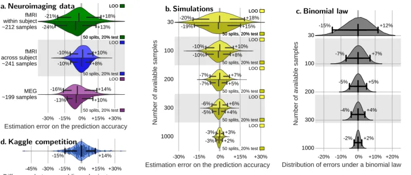
­30% ­15%  0% +15% +30%

Estimation error on the prediction accuracy       

fMRI within subject ~212 samples fMRI across subject ~241 samples MEG ~199 samples ­16%_{­13% +10%}+14% ­10% +8% ­10% +10% ­24% +13% ­21% +18% LOO 50 splits, 20% test LOO 50 splits, 20% test LOO 50 splits, 20% test LOO 50 splits, 20% test a. Neuroimaging data ­45% ­30% ­15%  0% +15% +30%

Difference between public and private scores       

­15% +14% d. Kaggle competition ­30% ­15%  0% +15% +30%

Estimation error on the prediction accuracy       

30 100 200 300 1000

Number of available samples   

­19% +15% ­20% +18% ­10% +8% ­10% +10% ­7% +5% ­7% +7% ­5% +4% ­6% +6% ­3%­3% +2%+3% LOO 50 splits, 20% test LOO 50 splits, 20% test LOO 50 splits, 20% test LOO 50 splits, 20% test LOO 50 splits, 20% test LOO 50 splits, 20% test b. Simulations ­20% ­10%  0% +10% +20%

Distribution of errors under a binomial law      

1000 300 200 100 30

Number of available samples   

­2% +2% ­4% +4% ­5% +5% ­7% +7% ­15% +12% c. Binomial law

Figure 1: Cross-validation errors. a – Distribution of errors between the prediction accuracy as assessed via cross-validation (average across folds) and as measured on a large independent test set for different types of neuroimaging data. Results fromVaroquaux et al.(2017) (seeAppendix B) b – Distribution of errors between the prediction accuracy as assessed via cross-validation on data of various sample sizes and as measured on 10 000 new data points for simple simulations (seeAppendix C). c – Distribution of errors as given by a binomial law: difference between the observed prediction error and the population value of the error, p = 75%, for different sample sizes. d – Discrepancies between private and public score. Each dot represents the difference between the accuracy of a method on the public test data and on the private one. The scores are retrieved fromwww.kaggle.com/c/mlsp-2014-mri, in which 144 subjects were used total, 86 for training the predictive model, 30 for the public test set, and 28 for the private test set. The bar and whiskers indicate the median and the 5th_{and 95}th

percentile. Measures on cross-validation (a and b) are reported for two reasonable choices of cross-validation strategy: leave one out (leave one run out or leave one subject out in data with multiple runs or subjects), or 50-times repeated splitting of 20% of the data.

the prediction accuracy measured by cross-validation and the expected accuracy on new data.

Previous results: cross-validation on brain images.

Varoquaux et al. (2017) used a nested cross-validation on neuroimaging data to measure this discrepancy: we split the data multiple times and compared errors (see Ap-pendix B). The strength of such an experiment is that it is applied on actual neuroimaging data, mimicking us-age by practitioners. Its weakness is that the models’ true generalization accuracy is not known and must be esti-mated.

Figure 1a summarizes the resulting cross-validation er-rors, show a similar behavior across different reasonable choices of cross-validation strategy: the common leave-one-run-out, and the recommended random splitting strat-egy (Varoquaux et al., 2017). The 5th and 95th per-centile of the distribution of errors are of particular in-terest as they correspond to the commonly accepted .05 threshold on p-values. The results show that these confi-dence bounds extends at least 10% both ways, regardless of the cross-validation strategy used. It implies that, when computing a given cross-validated accuracy, there is a 5% chance that it is 10% above the true generalization accu-racy, and a 5% chance this it is 10% below.

Spread out predictions in a public challenge. There could be something unusual in the settings of Varoquaux

et al.(2017). To reflect common practice in neuroimaging, I have inspected the results of a public prediction challenge (Silva et al., 2014) on the Kaggle website1. The compe-tition –predicting Schizophrenia diagnosis from functional and structural MRI– reports two accuracy measures esti-mated on a public (n = 30) and a private (n = 28) test set.

The accuracy scores reported on the public and the private test set show a large difference. Figure 1d summa-rizes these differences. Computing confidence bounds from these discrepancies gives errors on the order of ±15%. As neither the public nor the private test set is a gold stan-dard, it is reasonable to assume that errors are shared be-tween the two scores, and thus the actual margin of error on a single measurement is smaller by a factor of two. Simple simulations also display large error bars. To understand better the origin of these discrepancies, I used simple simulations: fitting a linear SVM on a two-class dataset, samples drawn i.i.d. from two Gaussian dis-tributions with a separation tuned such that the classifier achieves 75% accuracy. I then compare the prediction ac-curacy measure by cross-validation on these data with the accuracy that the classifier achieved on a large amount (10 000) new samples drawn from the same distribution.

1

An important benefit of this experiment is that it shows the difference between the cross-validation measure of the classifier’s accuracy, and the true generalization accuracy.

Figure 1b shows the resulting distribution of errors on the prediction accuracy estimated by cross validation for different size of the data available. For 100 samples, these experiments reproduces well the errors observed on neu-roimaging data (Figure 1a and 1d). Both leave one out and more sophisticated cross-validation strategies display large error bars2. As the sample size of the simulated data goes up, the error bars narrow markedly.

Intrinsically large sampling noise. The data clearly shows that the accuracy of predictive models is not well measured in neuroimaging. The small sample sizes en-countered in neuroimaging indeed make this task very challenging: as I show below, even in ideal situations, there is a large sampling noise in the measure.

The typical sample size of neuroimaging studies is less than 100 observations given to the classifier, trials or sub-jects depending on the settings (Figure 2). The simplest model for the observed prediction errors is that of toss-ing a coin 100 times with a probability p of success at each toss. The probability p corresponds to the accuracy of the classifier that we are trying to measure. The dis-tribution of number of successes is then given by a bi-nomial law (Pereira and Botvinick, 2011; Stelzer et al.,

2013). With 100 tosses, associated confidence bounds lie ±7% away from the true accuracy p (see Figure 1c).

This binomial law is a best-case scenario for errors on the accuracy measure: observations are i.i.d. and there is no additional variability from training a decoder. On the opposite, neuroimaging data is strife with correlation across samples and confounding effects, e.g. the temporal structure of trials or samples drawn either from the same subject or different subjects. These reduce the statisti-cal degrees of freedom and create an intrinsic variance in the prediction accuracy (Saeb et al., 2017; Little et al.,

2017). This is why we observe that cross-validation has larger errors on neuroimaging data (Figure 1a) than on the simulations (Figure 1b) or with the ideal binomial law (Figure 1c).

Simulations and a simple null model therefore show that the error bars of cross-validation observed in neu-roimaging are perfectly expected given the sample sizes. Improvements on cross-validation such as the reusable holdout (Dwork et al., 2015) cannot circumvent intrinsic limitations of small samples (seeAppendix A).

2_{Performing 50 repeated splits of 20% of the data yields slightly}

smaller error bars than leave one out, and can be significantly less computationally expensive for large datasets. This cross-validation strategy should be preferred, but will not fix the problem of large error bars.

5to 15 15to 50 50to 150 150to 500 500

_{to 1500 1500}

_{to 5000}

Number of available samples

Number of studies

Woo2017: Autism Woo2017: Depression Woo2017: Psychosis Woo2017: Alzheimer's Arbabshirani2017: Schizophrenia Arbabshirani2017: Alzheimer's Brown2017: Connectome learning Wolfer2015: psychiatric diagnostic Pubmed search "fmri decoding"

Figure 2: Sample sizes in neuroimaging studies A stacked histogram compounding sample sizes from multiple sources: the

Woo et al.(2017) review paper, differentiating Autism, Depression, Pyschosis, and Alzheimer’s studies, theArbabshirani et al. (2017) review paper, differentiating Schizophrenia and Alzheimer’s studies, theBrown and Hamarneh(2016) review on prediction from connec-tomes, and theWolfers et al.(2015) review on prediction for psychi-atric disorders, as well as the 100 first answers to a pubmed search on ”fmri decoding”. The total histogram comprises 642 studies, with a median number of samples of 89.

Note that I did not consider groups of less than 25 studies, and hence did not break up into pathologies theBrown and Hamarneh(2016) andWolfers et al.(2015) reviews.

2.2. Small sample sizes undermine statistical control Underestimated errors. Not only are the errors of cross-validation large, but it is also easy to underestimate them, as when using as a null the binomial distribution.

The simplest approach to put error bars on cross-validation results is to look at the dispersion of the predic-tion accuracy across the folds. However as the predicpredic-tions are not independent across folds, estimates of the vari-ance or related statistical tests are optimistic (Bengio and Grandvalet,2004). On the simulated data, formulas based on the standard error to mean underestimate confidence bounds by a factor of 0.7 in the best case (Appendix D). Permutation testing gives good statistical control on the prediction accuracy (Stelzer et al., 2013). Literature search on Google Scholar3 _{suggest that around a 30% of}

the publications on MVPA (mostly searchlight-based anal-ysis) use permutations, but that only 15% of the fMRI decoding studies use permutations.

Vibration effects. Analytic pipelines come with vari-ous methodological choices that are hard to settle a priori (Carp,2012). With a high-variance test statistic, as cross validation on few samples, methodological choices can have a drastic impact on the outcome of the analysis. This is sometimes known as vibration, and the key quantity is the ratio between the effect size and the variations due to analytical choices (Ioannidis, 2008). I explored vibration effects in decoding using the face versus place opposition in the Haxby et al. (2001) data. I inverted the labels to predict in one session out of two, to create a dataset in

3_{Pubmed does not do full-text search. On Google scholar, a search}

for“fmri decoding”in the last 5 years returned 15 500 results, while

“fmri decoding permutation”returned 2380; similarly,“fmri mvpa”

return 2360 results while“fmri mvpa permutation”return 728.

30%

40%

50%

60%

70%

Cross­validation scores for different decoders      

4 first

4 last

6 first

6 last

all 12

Sessions used 

25% 39% 40% 71% 38% 57% 47% 57% 44% 52% n~72 n~72 n~108 n~108 n~216

Figure 3: Different decoders on fMRI with permuted labels On each line shows the distribution of cross-validation scores for a va-riety of decoders (SVC and logistic regression, with different amount of univariate feature selection and spatial smoothing); a dot is the cross-validation score for one choice of decoder. These are applied to the fMRI data of the first subject inHaxby et al.(2001), discrim-inating face viewing and place viewing, but with labels inverted one session out of two; hence the expected accuracy is chance: 50%.

which fMRI should not predict the experimental condi-tion. On this data, I ran a variety of classic decoding pipelines, namely SVM or logistic regression, optionally with feature selection of 100, 200, 500, 1 000, or 2 000 vox-els and smoothing at 2, 4, or 6 mm. These are standard choices, but they give altogether almost 50 different re-lated decoding pipelines. I applied all these pipelines to various subsets of the data: the full 12 sessions, the 6 first or 6 last, or the 4 first or 4 last sessions.

Figure 3 shows the cross-validation scores obtained with the various pipelines. The expected prediction score is 50%, chance. When using all 12 sessions, the observed scores group well around 50%, with excursions ranging from 44% to 52%. However, when using less data the ex-cursions are much more pronounced, going up to 57% for 6 sessions and 71% for 4 sessions. In addition, the mean observed score varies notably across subsets of the data. Such variation can be explained by nonstationarities, e.g. fluctuation of attention of the subject, or sampling noise discussed above: the observations are very correlated and thus n ∼ 100 may not represent well the faces and places conditions.

3. Implications for neuroimaging

3.1. An open door to overfit and confirmation bias The large error bars are worrying, whether it is for methods development of predictive models or their use to study the brain and the mind. Indeed, a large variance of results combined with publication incentives weaken sci-entific progress (Ioannidis, 2005).

With conventional statistical hypothesis testing, the danger of vibration effects is well recognized: arbitrary degrees of freedom in the analysis explore the variance of the results and, as a consequence, control on false posi-tives is easily lost (Simmons et al., 2011). (Carp, 2012)

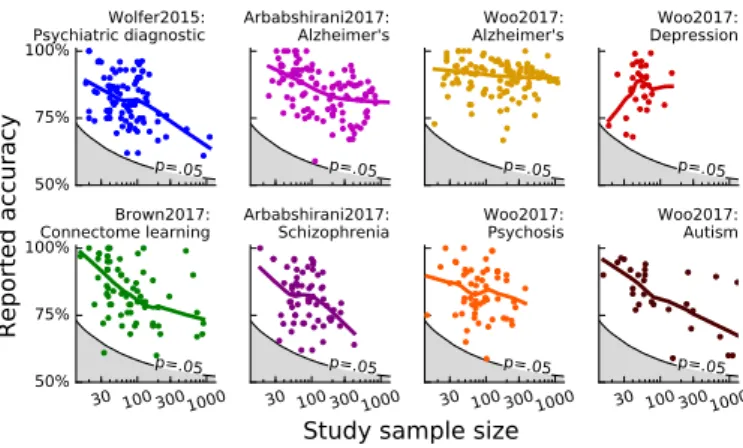
50% 75% 100% p=.05 Wolfer2015: Psychiatric diagnostic p=.05 Arbabshirani2017: _Alzheimer's p=.05 Woo2017: Alzheimer's p=.05 Woo2017: Depression 30 100 3001000 50% 75% 100% p=.05 Brown2017: Connectome learning 30 100 3001000 p=.05 Arbabshirani2017: Schizophrenia 30 100 3001000 p=.05 Woo2017: Psychosis 30 100 3001000 p=.05

Reported accuracy

Study sample size

Woo2017: Autism

Figure 4: Reported accuracy and sample size The various plots show reported prediction accuracy as a function of sample size for the studies in different the reviews considered inFigure 2. The black line and grey area represent the p = 0.05 threshold with a binomial null model, which, as shown in the results section, is likely to be op-timistic. The lines are Lowess fit to the data: robust non-parametric local regression.

has found that the variety of analytics choices is such in fMRI that almost every publication uses a unique pipeline. In predictive models, arbitrary choices can leads to artifi-cial improvements in the prediction accuracy measured by cross-validation (seesection 2.2andSkocik et al.(2016)). The larger is the variance of the measure of the prediction score, the larger are these effects. The improvements are meaningless as they will not carry over to predicting on new data. The danger is well known in machine learn-ing, where it is known as overfit. The standard remedy is to keep a large independent test set. However it is diffi-cult in neuroimaging, where data acquisition is costly. To mitigate such intrinsic problems, clinical trials often use blind analysis where part of the labels are unknown to the statistician.

Scientific publishing makes things worse: the literature acts as a filter as only studies that report significant effects are published. Such selective reporting can further under-mine control of the fraction of false detections in a body of literature (Rosenthal,1979). It also tends to inflate the reported effect size (Vul et al.,2009). An additional a dan-gerous effect of large variance is that it enables and justifies confirmation bias in publications: investigators or review-ers are more likely to publish results that are in agreement with their theory. Analysis of the literature suggests that publications are indeed too often on the edge of signifi-cance (Szucs and Ioannidis, 2016) and are vastly biased by selection according to the prevailing opinions ( Ioanni-dis,2008).

The combination of large variance and the filter effect of publications could explain why the prediction accuracy reported in publication often decreases as sample sizes in-crease. Indeed, inFigure 4I plot an meta analysis uniting the results discussed in several review papers. Each of these review select a variety of studies on different criteria such as methodology used or pathology studied. Overall,

the typical prediction accuracy reported in studies with small samples size is larger that reported in studies with many samples4_{. Homogeneity of the population and the}

imaging data is harder to control on larger cohorts. Hence uncontrolled heterogeneity might explain such a decrease. However, very few studies have compared large heteroge-neous cohorts to smaller well-controlled group with the same analytic pipeline. A notable exception, Abraham et al.(2017), finds that pooling data across sites leads to better predictive biomarkers of Autism, although this is a highly-heterogeneous spectrum disorder.

3.2. Cross-validation is nonetheless a crucial tool Cross-validation is not a silver bullet. However, it is the best tool available, because it is the only non-parametric method to test for model generalization. Bayesian ap-proaches such as Bayesian model selection or Bayesian model averaging rely on model evidence to test or select models (Penny et al., 2007, chap. 35). However, they are strongly parametric: the statistical control or the useful-ness of this test collapses if the modeling assumptions are wrong. Additionally, these approaches do not measure the ability of the model to predict on new data.

Testing for generalization is central to diagnostics or prognosis applications, where prediction is indeed the question. It has also a broader importance as the abil-ity to generalize findings is central to scientific investiga-tions. Research in psychology and neuroscience has fo-cused on explaining data, to seek causal mechanisms us-ing tightly-controlled experiments, eg based on randomiza-tion. However, too strong a focus on well-controlled expla-nation may limit the generality of the results (Yarkoni and Westfall,2016). The essential aspect of cross-validation is that it tests a model on observations independent from the data that was used to fit the model. This is the only assumption-free way to bound model complexity. In-deed, more complex model will always fit the data better. There are statistical procedures to set model complexity, such as Bayesian information criterion (BIC) and the re-lated Akaike information criterion (AIC) and minimum descriptor length (MDL). However, they rely on model-ing assumption such as data distribution, independence of the observations, and need much more observations than model parameters (Hastie et al., 2009, sec. 7.5).

3.3. Looking forward: some recommendations

Predictive models can extract richer and finer infor-mation from the complex data provided by brain imag-ing. However, best practices need to be adapted to en-sure enough statistical power to test these models. While larger datasets are certainly desirable, they are difficult and costly to acquire. At the subject level, data accumu-lation is limited by fatigue of the subject in the scanner

4_{Depression studies, as reported byWoo et al.(2017) do not show}

this decrease, however none of these have a large sample.

as well as habituation effects to the paradigm. Scanning many subjects may entails operational budgets beyond that typical of a neuroimaging grant. Nevertheless, there are a variety of solutions feasible without major changes in the field.

Data sharing and pooling, despite heterogeneity. Reusing shared data across investigators can increase sam-ple sizes while keeping bounds on data-acquisition costs (Poldrack and Gorgolewski,2014). Platforms to share neu-roimaging data are rapidly growing, as with OpenfMRI (Poldrack et al., 2013) that now hosts 63 studies com-prising 2 200 subjects, or Neurovault (Gorgolewski et al.,

2015) with 26 000 brain maps in 1 100 collection. Such sharing is easiest with harmonized protocols and conven-tions. Yet, outside of concerted efforts, there is a mas-sive amount of data potentially available: around 30 000 studies using fMRI are published each year5, many with new data. They answer a wide variety of different ques-tions; still they have some overlap. This overlap provides opportunity for reuse, increasing sample size. For cogni-tive neuroimaging, joint analysis is challenging due to the high specificity of cognitive questions studied. However, the success of meta-analysis in fMRI suggests that pooling data can be beneficial, whether it is by assembling a small number of well-matched studies or over a wider coverage of the literature (Laird et al.,2005;Costafreda,2009). In a remarkable example of predictive models using pooled data, Wager et al. (2013) were able to combine multiple pain studies to extract a neural signature specific to phys-ical pain, discriminating it from social pain or warmth.

To pool studies of brain pathologies, it is often easier to define a common covariate to predict across subjects, typ-ically a diagnostic status. However, studies of the same pathology can differ in their inclusion criteria, introduc-ing heterogeneity that confounds predictions or interpre-tations. Heterogeneity may be a challenge to the clini-cal relevance of studies on heterogeneous groups, as many neuro-psychiatric diseases are spectrum disorders that are likely composed of several forms of the disease. However, biomarkers that are too specific to a certain site or a cer-tain cohort have reduced clinical value (Woo et al.,2017). There are many documented successes of prediction from heterogeneous brain imaging data. For anatomical mark-ers of aging, Ziegler et al. (2014) show that using data from many scanners enables to generalize to new scanner.

Yahata et al. andAbraham et al. (2017) show that, for a disorder as heterogeneous as Autism, predicting diagnos-tic status across sites was possible. Moreover, Abraham et al.(2017) andDansereau et al.(2017) show that with a large number of sites, prediction across sites performed as well as prediction across subjects in the same site. Cross-validation on heterogeneous data requires some care, as prediction may be driven by a confounding covariate ( Lit-tle et al.,2017). For instance, when predicting with several

5_{As estimated from a PubMed search on fMRI.}

sessions per subject, care must be taken to avoid having different sessions of the same subject in the train and test set, to prevent subject-identification to be driving predic-tion (Saeb et al.,2017).

Paradigms facilitating larger data. Some experimen-tal paradigms make it easier to accumulate data, of-ten to the cost relinquishing fine control on cognition. For instance, to study cognition, standard localizer-type paradigms (Saxe et al.,2006) can easily be shared across many acquisitions, leading to large databases (Pinel et al.,

2007). Naturalistic stimuli enables faster presentations for longer times without fatigue of the subject. Therefore they can be used to accumulate subjects’ responses for rich de-coding studies (Kay et al.,2008). To study inter-individual differences, acquisition protocols that are comparatively universal and easy to acquire lead to large sample sizes. For instance there are more standard T1 maps available than myelin maps. In functional imaging, resting-state fMRI acquisition are a promising source of very large data, via post-hoc aggregation (Biswal et al., 2010; Thompson et al., 2014; Di Martino et al., 2014) or large concerted efforts (Miller et al., 2016; Van Essen et al., 2013). Cognitive neuroimaging results: at the group level. In cognitive neuroimaging, multi-voxel pattern analysis (MVPA) generally performs cross-validation across trials in the same subject. The number of trials cannot always be easily extended, due to habituation effects or limited time in the scanner. A more promising avenue to increase sample size is to exploit the replication of these decoding results across subjects. As there is significant variabil-ity in cognitive strategy or performance across subjects, pooling across subjects raises concerns. Yet, conclusions should be drawn from the group, and not at the subject level, where the small sample size tends to compromise cross-validation. There are several approaches. First, as outlined inStelzer et al.(2013) even when cross-validation is performed at the subject level, testing for significance of predictions can be done at the group level. This approach is used by a good fraction of the MVPA studies. Another option is to predict across subjects. This requires fine-grain matching of subjects’ anatomy and function, yet it bears the promise of more general representations of cog-nition (Haxby et al.,2011).

Evaluating methods on multiple studies. For meth-ods development, the vibration effects observed on Fig-ure 3are very troublesome. Indeed, the empirical work in methods development often amounts to trying out multi-ple approaches and publishing the one that works best. It leads naturally to overfit if the data are not large enough to guarantee errors on the measurement prediction accuracy smaller than the difference between methods. As I outline insection 2.2andAppendix D), it is hard to measure these error bars and they are usually underestimated. The best way to compare approaches without loophole is to test

Sample size 30 100 300 1000

Confidence bounds ±15% ±10% ±6% ±3% Table 1: Confidence bounds to be expected for a binary clas-sification, summarizing experiments and simulations inFigure 1. Actual confidence bounds may be significantly larger in adverse sit-uations such as with correlated observations or very unstable classi-fiers.

them across several datasets (Demˇsar, 2006). With the sample size typical of neuroimaging, I personally believe that this is the only sound way of doing methods devel-opment. As most methods researchers, I have not always worked like this in the past, and some of the promising results that we have published have not carried over6.

4. Conclusion: improving predictive neuroimaging

With predictive models even more than with standard statistics small sample sizes undermine accurate tests. The problem is inherent to the discriminant nature of the test, measuring only a success or failure per observations. Esti-mates of variance across cross-validation folds give a false sense of security as they strongly underestimates errors on the prediction accuracy: folds are far from independent. Rather, to avoid the illusion of biomarkers that do not gen-eralize or overly-optimistic methods development, ballpark estimates of confidence bounds summarized inTable 1may be more useful. A typical sample size in neuroimaging, 100 observations, leads to ±10% errors in prediction accuracy. Cognitive neuroscience MVPA studies often control these errors by performing a group-level statistical analysis.

Exploring arbitrary choices in analytic pipelines eas-ily creates improvements in measured prediction accu-racy that will not generalize to new data. Such effect is a major impediment for methods development as it be-comes challenging to ensure that improvements observed are meaningful. Due to the specificities of datasets, proto-cols, or pathologies, there cannot be a one-size-fits-all op-timal method for predictive modeling. However, to limit the variety of analytics pipelines, we, methods developers, must provide general recommendations validated on many datasets.

With small sample sizes, research with predictive mod-els is performed blindfolded. The problem is neither new nor specific to neuroimaging. In genomics,Braga-Neto and Dougherty(2004) have asked “Is cross-validation valid for small-sample microarray classification?”. In neuroimag-ing, it is magnified by the intrinsic difficulty of acquiring large datasets. The problem will not be fixed by better classifiers or cross-validation approaches. Solutions will lie in approaches using larger samples sizes or preregistered

6_{As an example, we were not able to reproduce the benefits of the}

specific algorithm inMichel et al.(2012) on other datasets, though we later validated some of the core ideas –voxel clustering– on many other datasetsVaroquaux et al.(2012);Hoyos-Idrobo et al.(2016).

analyses. Overall, exploring larger datasets is a promis-ing future for neuroimagpromis-ing (Poldrack et al.,2017). Their richness is best captured by multivariate models (Miller et al.,2016). For predictive applications such as biomark-ers, larger datasets lead to better prediction on hard prob-lems, even in the face of increased variability.

Acknowledgments

Computing resources were provided by the NiConnect project (ANR-11-BINF-0004 NiConnect). I am grateful to Aaron Schurger, Steve Smith, and Russell Poldrack for feedback on the manuscript. I would also like to thank Alexandra Elbakyan for help with the literature review, as well as Colin Brown and Choong-Wan Woo for sharing data of their review papers.

References

Abraham, A., Milham, M.P., Di Martino, A., Craddock, R.C., Sama-ras, D., Thirion, B., Varoquaux, G., 2017. Deriving reproducible biomarkers from multi-site resting-state data: An autism-based example. NeuroImage 147, 736–745.

Arbabshirani, M.R., Plis, S., Sui, J., Calhoun, V.D., 2017. Single subject prediction of brain disorders in neuroimaging: Promises and pitfalls. NeuroImage 145, 137–165.

Arlot, S., Celisse, A., 2010. A survey of cross-validation procedures for model selection. Statistics surveys 4, 40.

Bengio, Y., Grandvalet, Y., 2004. No unbiased estimator of the variance of k-fold cross-validation. Journal of machine learning research 5, 1089.

Biswal, B., Mennes, M., Zuo, X., Gohel, S., Kelly, C., Smith, S., Beckmann, C., et al., 2010. Toward discovery science of human brain function. Proc Ntl Acad Sci 107, 4734.

Braga-Neto, U.M., Dougherty, E.R., 2004. Is cross-validation valid for small-sample microarray classification? Bioinformatics 20, 374–380.

Brown, C.J., Hamarneh, G., 2016. Machine learning on human con-nectome data from mri. arXiv:1611.08699 .

Button, K.S., Ioannidis, J.P., Mokrysz, C., Nosek, B.A., Flint, J., Robinson, E.S., Munaf`o, M.R., 2013. Power failure: why small sample size undermines the reliability of neuroscience. Nature Reviews Neuroscience 14, 365–376.

Carp, J., 2012. The secret lives of experiments: methods reporting in the fmri literature. Neuroimage 63, 289–300.

Costafreda, S.G., 2009. Pooling fmri data: meta-analysis, mega-analysis and multi-center studies. Frontiers in neuroinformatics 3, 33.

Dansereau, C., Benhajali, Y., Risterucci, C., Pich, E.M., Orban, P., Arnold, D., Bellec, P., 2017. Statistical power and prediction accuracy in multisite resting-state fmri connectivity. NeuroImage 149, 220–232.

Demˇsar, J., 2006. Statistical comparisons of classifiers over multiple data sets. Journal of Machine learning research 7, 1–30.

Di Martino, A., Yan, C.G., Li, Q., Denio, E., Castellanos, F.X., Alaerts, K., Anderson, J.S., Assaf, M., Bookheimer, S.Y., Dapretto, M., et al., 2014. The autism brain imaging data ex-change: towards a large-scale evaluation of the intrinsic brain ar-chitecture in autism. Molecular psychiatry 19, 659–667.

Dwork, C., Feldman, V., Hardt, M., Pitassi, T., Reingold, O., Roth, A., 2015. The reusable holdout: Preserving validity in adaptive data analysis. Science 349, 636.

Gorgolewski, K.J., Varoquaux, G., Rivera, G., Schwarz, Y., Ghosh, S.S., Maumet, C., Sochat, V.V., Nichols, T.E., Poldrack, R.A., Poline, J.B., et al., 2015. Neurovault. org: a web-based repository for collecting and sharing unthresholded statistical maps of the human brain. Frontiers in neuroinformatics 9, 8.

Hastie, T., Tibshirani, R., Friedman, J., 2009. The elements of sta-tistical learning. Springer.

Haxby, J.V., Gobbini, I.M., Furey, M.L., et al., 2001. Distributed and overlapping representations of faces and objects in ventral temporal cortex. Science 293, 2425.

Haxby, J.V., Guntupalli, J.S., Connolly, A.C., Halchenko, Y.O., Con-roy, B.R., Gobbini, M.I., Hanke, M., Ramadge, P.J., 2011. A common, high-dimensional model of the representational space in human ventral temporal cortex. Neuron 72, 404–416.

Haynes, J.D., Rees, G., 2006. Decoding mental states from brain activity in humans. Nat. Rev. Neurosci. 7, 523.

Hoyos-Idrobo, A., Varoquaux, G., Kahn, J., Thirion, B., 2016. Re-cursive nearest agglomeration (rena): fast clustering for approx-imation of structured signals. arXiv preprint arXiv:1609.04608 .

Ioannidis, J.P., 2005. Why most published research findings are false. PLos med 2, e124.

Ioannidis, J.P., 2008. Why most discovered true associations are inflated. Epidemiology 19, 640–648.

Kay, K.N., Naselaris, T., Prenger, R.J., Gallant, J.L., 2008. Iden-tifying natural images from human brain activity. Nature 452, 352–355.

Kriegeskorte, N., Goebel, R., Bandettini, P., 2006. Information-based functional brain mapping. Proceedings of the National Academy of Sciences of the United States of America 103, 3863. Laird, A.R., Fox, P.M., Price, C.J., Glahn, D.C., Uecker, A.M.,

Lan-caster, J.L., Turkeltaub, P.E., Kochunov, P., Fox, P.T., 2005. Ale meta-analysis: Controlling the false discovery rate and performing statistical contrasts. Human brain mapping 25, 155–164. Little, M.A., Varoquaux, G., Saeb, S., Lonini, L., Jayaraman, A.,

Mohr, D., Kording, K.P., 2017. Using and understanding cross-validation strategies. perspectives on Saeb et al. GigaScience , in press.

Michel, V., Gramfort, A., Varoquaux, G., Eger, E., Keribin, C., Thirion, B., 2012. A supervised clustering approach for fmri-based inference of brain states. Pattern Recognition 45, 2041–2049. Miller, K.L., Alfaro-Almagro, F., Bangerter, N.K., Thomas, D.L.,

Yacoub, E., Xu, J., Bartsch, A.J., Jbabdi, S., Sotiropoulos, S.N., Andersson, J.L., et al., 2016. Multimodal population brain imag-ing in the uk biobank prospective epidemiological study. Nature Neuroscience .

Nishimoto, S., Vu, A.T., Naselaris, T., Benjamini, Y., Yu, B., Gal-lant, J.L., 2011. Reconstructing visual experiences from brain activity evoked by natural movies. Current Biology 21, 1641. Norman, K.A., Polyn, S.M., Detre, G.J., Haxby, J.V., 2006. Beyond

mind-reading: multi-voxel pattern analysis of fMRI data. Trends in cognitive sciences 10, 424.

Penny, W.D., Friston, K.J., Ashburner, J.T., Kiebel, S.J., Nichols, T.E., 2007. Statistical Parametric Mapping: The Analysis of Functional Brain Images. Academic Press, London.

Pereira, F., Botvinick, M., 2011. Information mapping with pattern classifiers: a comparative study. Neuroimage 56, 476.

Pereira, F., Mitchell, T., Botvinick, M., 2009. Machine learning classifiers and fMRI: a tutorial overview. Neuroimage 45, S199. Pinel, P., Thirion, B., Meriaux, S., Jobert, A., Serres, J., Le Bihan,

D., Poline, J.B., Dehaene, S., 2007. Fast reproducible identifica-tion and large-scale databasing of individual funcidentifica-tional cognitive networks. BMC neuroscience 8, 91.

Poldrack, R., Baker, C.I., Durnez, J., Gorgolewski, K., Matthews, P.M., Munafo, M., Nichols, T., Poline, J.B., Vul, E., Yarkoni, T., 2017. Scanning the horizon: Future challenges for neuroimaging research. Nature Reviews Neuroscience 18, 115.

Poldrack, R.A., Barch, D.M., Mitchell, J., Wager, T., Wagner, A.D., Devlin, J.T., Cumba, C., Koyejo, O., Milham, M., 2013. Toward open sharing of task-based fmri data: the openfmri project. Fron-tiers in neuroinformatics 7, 12.

Poldrack, R.A., Gorgolewski, K.J., 2014. Making big data open: data sharing in neuroimaging. Nature neuroscience 17, 1510–1517. Poldrack, R.A., Halchenko, Y.O., Hanson, S.J., 2009. Decoding the

large-scale structure of brain function by classifying mental states across individuals. Psychological Science 20, 1364.

Rosenthal, R., 1979. The file drawer problem and tolerance for null results. Psychological bulletin 86, 638.

Saeb, S., Lonini, L., Jayaraman, A., Mohr, David andKording, K.P., 2017. The need to approximate the use-case in clinical machine learning. GigaScience , in press.

Saxe, R., Brett, M., Kanwisher, N., 2006. Divide and conquer: a defense of functional localizers. Neuroimage 30, 1088–1096. Silva, R.F., Castro, E., Gupta, C.N., Cetin, M., Arbabshirani, M.,

Potluru, V.K., Plis, S.M., Calhoun, V.D., 2014. The tenth an-nual mlsp competition: schizophrenia classification challenge, in: Machine Learning for Signal Processing (MLSP), 2014 IEEE In-ternational Workshop on, IEEE. pp. 1–6.

Simmons, J.P., Nelson, L.D., Simonsohn, U., 2011. False-positive psychology: Undisclosed flexibility in data collection and analysis allows presenting anything as significant. Psychological science 22, 1359.

Skocik, M., Collins, J., Callahan-Flintoft, C., Bowman, H., Wyble, B., 2016. I tried a bunch of things: the dangers of unexpected overfitting in classification. bioRxiv , 078816.

Smith, S.M., Nichols, T.E., Vidaurre, D., Winkler, A.M., Behrens, T.E., Glasser, M.F., Ugurbil, K., Barch, D.M., Van Essen, D.C., Miller, K.L., 2015. A positive-negative mode of population covari-ation links brain connectivity, demographics and behavior. Nature neuroscience 18, 1565–1567.

Stelzer, J., Chen, Y., Turner, R., 2013. Statistical inference and mul-tiple testing correction in classification-based multi-voxel pattern analysis (mvpa): random permutations and cluster size control. Neuroimage 65, 69–82.

Szucs, D., Ioannidis, J.P., 2016. Empirical assessment of published effect sizes and power in the recent cognitive neuroscience and psychology literature. bioRxiv , 071530.

Thompson, P.M., Stein, J.L., Medland, S.E., Hibar, D.P., Vasquez, A.A., Renteria, M.E., Toro, R., Jahanshad, N., Schumann, G., Franke, B., et al., 2014. The enigma consortium: large-scale collaborative analyses of neuroimaging and genetic data. Brain imaging and behavior 8, 153–182.

Van Essen, D.C., Smith, S.M., Barch, D.M., Behrens, T.E., Yacoub, E., Ugurbil, K., Consortium, W.M.H., et al., 2013. The wu-minn human connectome project: an overview. Neuroimage 80, 62–79. Varoquaux, G., Gramfort, A., Thirion, B., 2012. Small-sample brain mapping: sparse recovery on spatially correlated designs with ran-domization and clustering. ICML , 1375.

Varoquaux, G., Raamana, P.R., Engemann, D.A., Hoyos-Idrobo, A., Schwartz, Y., Thirion, B., 2017. Assessing and tuning brain de-coders: cross-validation, caveats, and guidelines. NeuroImage 145, 166–179.

Varoquaux, G., Thirion, B., 2014. How machine learning is shaping cognitive neuroimaging. GigaScience 3, 28.

Vul, E., Harris, C., Winkielman, P., Pashler, H., 2009. Puzzlingly high correlations in fmri studies of emotion, personality, and social cognition. Perspectives on psychological science 4, 274.

Wager, T.D., Atlas, L.Y., Lindquist, M.A., Roy, M., Woo, C.W., Kross, E., 2013. An fMRI-based neurologic signature of physical pain. New England Journal of Medicine 368, 1388.

Wolfers, T., Buitelaar, J.K., Beckmann, C.F., Franke, B., Marquand, A.F., 2015. From estimating activation locality to predicting disor-der: a review of pattern recognition for neuroimaging-based psy-chiatric diagnostics. Neuroscience & Biobehavioral Reviews 57, 328.

Woo, C.W., Chang, L.J., Lindquist, M.A., Wager, T.D., 2017. Build-ing better biomarkers: brain models in translational neuroimag-ing. Nature Neuroscience 20, 365–377.

Yahata, N., Morimoto, J., Hashimoto, R., Lisi, G., Shibata, K., Kawakubo, Y., Kuwabara, H., Kuroda, M., Yamada, T., Megumi, F., et al., . A small number of abnormal brain connections predicts adult autism spectrum disorder. NATURE 7, 1.

Yarkoni, T., Westfall, J., 2016. Choosing prediction over explanation in psychology: Lessons from machine learning. figshare preprint. Ziegler, G., Ridgway, G.R., Dahnke, R., Gaser, C., Initiative,

A.D.N., et al., 2014. Individualized gaussian process-based predic-tion and detecpredic-tion of local and global gray matter abnormalities

in elderly subjects. NeuroImage 97, 333–348.

Appendix A. Additional considerations on

uncer-tainty in prediction accuracy

Appendix A.1. The reusable holdout

Dwork et al.(2015) propose an elegant technique to reuse

a given holdout set while avoiding overfitting it. However, the technique relies on jittering the measure of prediction error when it is below a threshold7. The technique does not fix the intrinsic uncertainty in the measurement of the prediction accu-racy –a task likely impossible– but it embeds this uncertainty in the validation procedure, refusing to conclude beyond a thresh-old directly related to confidence intervals of the prediction

(Dwork et al.,2015, supp mat). A given control on

generaliza-tion performance requires setting the threshold proporgeneraliza-tional to √

n. The reusable holdout is a beautiful improvement to cross-validation, that is however aligned with the main point that I am making: measuring prediction accuracy is not reliable with small samples.

Appendix A.2. Confidence bounds for varying expected ac-curacy

The experiments performed so far are for a chance level of 50% and an average prediction accuracy of 75%. While these numbers are typical in many decoding experiments, some experiments probe multiclass decoding, sometimes with many classes, in which case the accuracy under chance as well as the observed accuracy may be much lower. In such situations, the mechanisms driving estimation errors in cross-validation are the same, hence a binomial law still give a lower-bound on the distribution of errors. The binomial must be adapted to be centered on the expected accuracy, whether it is to compute the null distribution or to evaluate confidence bounds on ob-served values. Figure A1shows different binomial distributions

7_{Technically, the jitter is performed when train and test errors are}

very close to each other. Optimally-tuned predictors strike a balance between over and under fit and hence have close error rates on the train and test set.

0% 20% 40% 60% 80% 100%

Distribution of errors under a binomial law

300 100 30

Number of available samples   

_{10% 25% 50% 75% 90%}

Figure A1: Varying expected accuracy Binomial distributions for varying expected accuracy and number of samples. These indicate the shape of sampling noise, whether it is for a null distribution or the observed values.

Expected 5%–95% confidence bounds

accuracy 30 samples 100 samples 300 samples 10.0% 3.3%–20.0% 5.0%–15.0% 7.3%–13.0% 25.0% 13.3%–40.0% 18.0%–32.0% 21.0%–29.0% 50.0% 36.7%–63.3% 42.0%–58.0% 45.3%–54.7% 75.0% 60.0%–86.7% 68.0%–82.0% 71.0%–79.0% 90.0% 80.0%–96.7% 85.0%–95.0% 87.0%–92.7%

Table A1: Confidence bounds for a varying expected accuracy and varying number of samples, the 5 and 95% percentile of the binomial distribution, giving a lower-bound on the confidence bounds as it is a conservative distribution of errors (see Figure A5). Not that experiments revealed that the binomial distribution underestimates errors, hence actual confidence bounds are likely to be higher.

for various values of expected accuracy and number of samples. For expected accuracy close to 0% or 100%, the distributions narrow and becomes asymmetric due to the censoring effect of these limits. With large sample sizes, the distributions are more narrow, and these effects are less visible. Table A1gives corre-sponding 5 and 95% confidence bounds and shows that indeed, the confidence bounds are tighter near 0% or 100% prediction accuracy.

Appendix B. Experiments of Varoquaux 2017

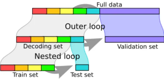
To facilitate reading this paper, I summarize here the ex-perimental protocol used inVaroquaux et al.(2017). The prin-ciple of the experiment is that the data are split twice (see

Fig-ure A2): first in a decoding set and a validation set; then

cross-validation is performed on the decoding set results in an esti-mate of prediction accuracy –as in any cross-validation based study–; finally this estimate is compared to the prediction ac-curacy of the models on the left-out validation set. To give a good measure of accuracy on the validation set, this set is taken large, as large as the decoding set. The estimation error of cross-validation is then measured by the discrepancy between the prediction accuracy on the validation set, and the predic-tion accuracy obtained by the cross-validapredic-tion procedure on the decoding set. Varoquaux et al.(2017) applied such exper-iments on a variety of neuroimaging decoding datasets, within and across subjects, in fMRI, VBM (Voxel Based Morphome-try) and MEG (Magneto EncephaloGraphy).

Validation set Full data Test set Train set Nested loop Outer loop Decoding set

Figure A2: Splitting the data twice: first in validation and decoding set, and then performing cross-validation on the decoding set.

Appendix C. Details on the simulations

Appendix C.1. Dataset simulation

I generate data with samples from two classes, each de-scribed by a Gaussian of identity covariance in 100 dimensions.

Figure A3: 2D view on simu-lated data The two classes are represented in red and blue cir-cles. Here, to simplify visualiza-tion, the data are generated in 2D (2 features), unlike the actual experiments, which are performed on 300 features.

X1

X2

The classes are centered respectively on vectors (µ, . . . , µ) and (−µ, . . . , −µ) where µ is a parameter adjusted to control the separability of the classes. With larger µ the expected pre-dictive accuracy would be higher. The samples are gener-ated i.i.d., with is a simplification compared to time-series, as in decoding, where there often is a dependence between neighboring observations, or in the same session. I chose the separability µ empirically to have a classification accuracy of

75%. Figure A3 shows a 2D view of the corresponding data.

Code to reproduce the simulations can be found on https:

//github.com/GaelVaroquaux/cross_validation_failure.

Appendix C.2. Experiments on simulated data

Unlike with a brain imaging datasets, simulations open the door to measuring the actual prediction performance of a classi-fier, and therefore comparing it to the cross-validation measure. For this purpose, I generate a pseudo-experimental data with a varying number of train samples, and a separate very large test set, with 10 000 samples. The train samples corre-spond to the data available during a neuroimaging experiment, and I perform cross-validation on these. I then apply the de-coder on the test set. The large number of test samples provides a good measure of prediction power of the decoder (Arlot and

Celisse,2010). As a decoder, I use a linear SVM with C=1,

as it is common in neuroimaging. To accumulate measures, I repeat the whole procedure 1000 times.

Appendix D. Results on the standard error of the

mean

A common approach to give error bars is to compute the standard error of the mean (SEM) across the cross-validation folds. For samples drawn from a normal distribution, the dis-tance from the mean of the upper and lower 95% confidence limit is given by 1.64 SEM 8. The SEM is also the quantity that appears in a T test. On the simulations, I compared such confidence limits computed from the SEM to the observed per-centile ofFigure A4.

Using the standard formula based on the SEM under-estimates actual confidence bounds by a factor of 0.73 for leave one out and 0.26 for repeated train-test split with 20% left out and 50 splits. There is indeed a wide difference is how much different folds are correlated in a cross-validation strat-egy. To give a more precise estimation of prediction accuracy, repeated random splits create more correlations across fold, and hence standard SEM computation that ignores this correlation is more severely incorrect.

8_{If the test is two-sided, the confidence bound are given by}

1.96 SEM. 9

 0%

+5%

+10% +15% +20%

95 percentile on the observed error      

 0%

+5%

+10%

+15%

+20%

95% confidence limit from SEM 

SEM over­estimates error bars SEM under­estimates error bars

Cross­validation

strategy

LOO

50 splits

20% test

CV train SEM empirical

strategy size error bar error bar

LOO 30 ±13.8% ±18.9% 100 ±7.4% ±10.3% 300 ±4.1% ±5.9% 1000 ±2.2% ±2.9% 50 splits, 20% test 30 ±3.4% ±15.3% 100 ±2.0% ±8.1% 300 ±1.1% ±4.1% 1000 ±0.6% ±2.1%

Figure A4: Error bars: SEM estimates versus observed In conventional models, the confidence limits are a factor 1.64 of the standard error of the mean (SEM). This figure represents such confi-dence limits on cross-validation estimated from SEM across the folds as a function of the actual estimation error observed in the simula-tions. Using the standard formula to compute the 95% confidence limit under-estimates it significantly compared to the actual 95 per-centile of the observed error, thought the two different choices of cross-validation strategy, leave one out, and 50-times repeated split-ting of 20% of the data, give different under-estimation: a factor of 0.73 for leave one out, and 0.26 for 50 repeat splits.

Appendix E. Experiments with the perfect

predic-tor

To fully rule out that the errors witnessed on cross-validation are due to instabilities of the predictive model, I re-peated the experiments with a predictor independent from the data. Specifically, I used the knowledge of the data-generating process to create a classifier making best decision possible. I then ran the cross-validation experiments with this classifier.

Figure A5 gives the corresponding distribution of mismatch

between the accuracy measured by cross-validation and the ac-tually accuracy of the classifier.

The results with the perfect predictor are very similar to those using an actual decoder trained on the data9 (Figure 1b using a linear SVM). Given that the classifier is independent of the data, the variability observed here can clearly be traced to sampling noise in the test set. Leave-one-out and random splits with 20% of the data give the same errors.

9_{Note that I set the separation in the data generation to have}

a prediction accuracy of 75%. As the perfect predictor is a better predictor than a linear SVC, experiments with the perfect predictor are done with a large separation.

­15% ­10% ­5%  0% +5% +10% +15%

Error on the estimation of prediction accuracy        

100 300 900

Number of available samples

­10% +8% ­11% +8% ­6% +6% ­6% +5% ­3% +3% ­3% +3% LOO 50 splits, 20% left out LOO 50 splits, 20% left out LOO 50 splits, 20% left out LOO 50 splits, 20% left out Perfect predictor

Figure A5: Cross-validation error with the perfect predictor. Given a data-independent optimal predictor, distribution of errors between the prediction accuracy as assessed via cross-validation on data of various sample sizes and the expected error of the predictor. The bar and whiskers indicate the median and the 5th_{and 95}th

per-centile. The distributions are reported for two reasonable choices of cross-validation strategy: leave one out, or 50-times repeated split-ting of 20% of the data.