Modeling Third Generation Neural Networks as Timed Automata and verifying their behavior through Temporal Logic

(1)

HAL Id: hal-01473941

https://hal.archives-ouvertes.fr/hal-01473941

Submitted on 22 Feb 2017

HAL is a multi-disciplinary open access

archive for the deposit and dissemination of sci-entific research documents, whether they are pub-lished or not. The documents may come from teaching and research institutions in France or

L’archive ouverte pluridisciplinaire HAL, est destinée au dépôt et à la diffusion de documents scientifiques de niveau recherche, publiés ou non, émanant des établissements d’enseignement et de recherche français ou étrangers, des laboratoires

Modeling Third Generation Neural Networks as Timed

Automata and verifying their behavior through

Temporal Logic

Giovanni Ciatto, Elisabetta de Maria, Cinzia Di Giusto

To cite this version:

Giovanni Ciatto, Elisabetta de Maria, Cinzia Di Giusto. Modeling Third Generation Neural Net-works as Timed Automata and verifying their behavior through Temporal Logic. [Research Report] Université Côte d’Azur, CNRS, I3S, France. 2017. �hal-01473941�

(2)

Modeling Third Generation

Neural Networks as Timed

Automata and verifying their

behavior through Temporal

Logic

Giovanni Ciatto

Elisabetta De Maria

Cinzia Di Giusto

(3)

Abstract

In this paper we present a novel approach to model Spiking Neural Networks. These networks, referred as third generation ones, add a new dimension to the second generation: the temporal axis. We propose a formalisation of Spiking Neural Networks based on Timed Automata Networks. Neurons are modelled as timed automata waiting for inputs on a number of different channels (synapses), for a given amount of time (the accumulation period). When this period is over, the current potential value is computed taking into account the current inputs and the previous decayed potential value. If the current potential overcomes a given threshold, the automaton emits a broad-cast signal over its output channel, otherwise it restarts another accumulation period. After each emission, the automaton is constrained to remain inactive for a fixed refractory period. Spiking neural networks are formalised as sets of automata, one for each neuron, running in parallel and sharing channels ac-cording to the structure of the network. The model is then validated against some properties defined via proper temporal logic formulae.

(4)

Chapter 1 Introduction

Researchers have been trying to reproduce the behavior of the brain for over half a century: on one side they are studying the inner functioning of neurons — which are its elementary components —, their interactions and how such aspects participate to the ability to move, learn or remember, typical of living beings, on the other side they are emulating nature trying to reproduce such capabilities e.g., within robot controllers, speech/text/face recognition applications etc.

In order to achieve a complete comprehension of the brain functioning, both neurons behavior and their interaction must be studied. Historically, interconnected neurons, “Neural Networks”, have been naturally modeled as directed weighted graphs where vertexes are computational units receiving inputs by a number of ingoing arcs, called synapses, elaborating it, and possibly propagating it over of outgoing arcs. Several inner models of the neuron behavior have been proposed: some of them make neurons behave as binary threshold gates, other ones exploit a sigmoidal transfer function, while, in a number of cases, differential equations are employed.

According to [17,20], three different and progressive generations of neu-ral networks can be recognized: (i) first generation includes discrete and threshold based models (e.g., McCulloch and Pitt’s neuron [19]); (ii) sec-ond generation consists of real valued and sigmoidal-based models, which are nowadays heavily employed in Machine Learning related tasks because of the existence of powerful learning algorithms (e.g., error

(6)

back-propaga-tion [22]); (iii) third generaback-propaga-tion, which is the focus of our work, consists of a number of model that, in addition to stimuli magnitude and differently from previous generations, take time into account.

Models from the third generation, also known as “Spiking Neural Net-works”, are weighted directed graphs where arcs represent synapses, weights serve as synaptic strengths, and vertexes correspond to “Spiking Neurons”. The latter ones are computational units that may emit (or fire) output im-pulses (spikes) taking into account input imim-pulses strength and their occur-rence instants. Models of this sort are of great interest not only because they are closer to natural neural networks behavior, but also because the tem-poral dimension allows to represent information according to various coding schemes [20,21]: e.g., the amount of spikes occurred within a given time window (rate coding), the reception/absence of spikes over different synapses (binary coding), the relative order of spikes occurrences (rate rank coding) or the precise time difference between any two successive spikes (timing code). A number of spiking neuron models have been proposed in literature, hav-ing different complexities and capabilities. In [14] spikhav-ing neuron models are classified according to some behaviors (i.e., typical responses to an input pattern) that they should exhibit in order to be considered biologically rel-evant. For example the Leaky Integrate & Fire (LI&F) model [15], where past inputs relevance exponentially decays with time, is one of the most studied neuron models because of its simplicity [14,20], while the Hodgkin-Huxley (H-H) model [11] is one of the most complex and important within the scope of computational neuroscience, being composed by four differen-tial equations comparing the neuron to an electrical circuit. Two behaviors that every model is able to reproduce are the tonic spiking and integrator : the former one describes neurons producing a periodic output if stimulated by a persistent input, the latter one illustrates how temporally closer input spikes have a greater excitatory effect on neurons potential, making them able to act as coincidence detectors. As one may expect, the more complex the model, the more behaviors it can be reproduce, at the price of greater computational cost for simulation and formal analysis; e.g., the H-H model can reproduce all behaviors, but the simulation process is really expensive even for just a few neurons being simulated for a small amount of time [14].

(7)

Our aim is to produce a neuron model being meaningful from a biological point of view but also amenable to formal analysis and verification, that could be therefore used to detect non-active portions within some network (i.e., the subset of neurons not contributing to the network outcome), to test whether a particular output sequence can be produced or not, to prove that a network may never be able to emit, or assess if a change to the network structure can alter its behavior; or investigate (new) learning algorithms which take time into account.

In this work, we take the discretized variant of LI&F introduced in [7] and we encode it into Timed Automata. We show how to define the behavior of a single neuron and how to build a network of neurons. Finally, we show how to verify properties of the designed system via Model Checking.

Timed Automata are Finite State Automata extended with timed be-haviors: constraints are allowed limiting the amount of time an automaton can remain within a particular state, or the time interval during which a particular transition may be enabled. Timed Automata Networks are sets of automata that can interact by means of channels.

Our modelling of Spiking Neural Network consists of a Timed Automata Networks where each neuron is an automaton alternating between two states: it accumulates the weighted sum of inputs, provided by a number of ingoing weighted synapses, for a given amount of time, and then, if the potential accu-mulated during the last and previous accumulation periods overcomes a given threshold, the neuron fires an output over the outgoing synapse. Synapses are channels shared between the TA representing neurons, while spike emissions are represented by synchronizations occurring over such channels. Timed Automata can be exploited to produce or recognize precisely defined spike sequences, too.

The biophysical behaviors mentioned above are interpreted as Computa-tional Tree Logic (CTL) formulae and are tested in Uppaal [3] that provides an extended modeling language for automata, a simulator for step-by-step analysis and a subset of CTL for systems verification.

The rest of the report is organized as follows: Chapter 2 exposes the theoretical background. It explains the differences between the three neural networks generations and describes our reference model, the Leaky Integrate

(8)

& Fire. It illustrates the expected behaviors. Finally it recalls definitions of Timed Automata Networks and Computational Tree Logics. Chapter

3 shows how Spiking Neural Networks are encoded into Timed Automata Networks, how inputs and outputs are handled by automata. Chapter 4

provides formal proofs for the behaviors listed above. Finally, Chapter 5

(9)

Chapter 2 Theoretical background

2.1 Neural Networks

Neural Networks are directed weighted graphs were nodes are computational units, also known as neurons, and edges represents synapses, i.e., connections between some neuron output and some other neuron input. Several models exist in literature and they differ on the signals that neurons emit/accept and on the way such signal are elaborated. An interesting classification has been proposed in [17] which distinguishes three different generations of Neural Networks:

1. network models within the first generation handle discrete inputs and outputs and their computational units are threshold-based transfer functions; this includes McCulloch and Pitt’s threshold gate [19], the perceptron [9], Hopfield networks [12] and Boltzmann machines [1]; 2. second generation models, instead, exploit real valued activation

func-tions, e.g., the sigmoid function, accepting and producing real values: a well known example is the multi-layer perceptron [6,22];

3. networks from the third generation are known as Spiking Neural Net-works. They extend second generation models treating time-dependent and real valued signals often composed by spike trains. Neurons may fire output spikes according to threshold-based rules which take into account input spikes magnitude and occurrence time [20].

(10)

The core of our analysis are Spiking Neural Networks. Because of the introduction of timing aspects (in particular, observe that information is represented not only by spikes magnitudes but also by their frequency) they are considered closer to the actual brain functioning than other generations models.

We adopt Maass’s definition (see [17] or [16]) because it is a widely gen-eral template which can be specialized in more fine-grained characterization by providing additional constraints. Spiking Neural Networks are modeled as directed weighted graphs where vertexes are computational units and edges represents synapses. The signals propagating over synapses are trains of im-pulses: spikes. The particular wave form of impulses must be specified by model instances. Synapses may modulate such signals according to their weight or they could introduce some propagation delay. Synapses are classi-fied according to their weight as excitatory, if it is positive, or inhibitory if negative.

Computational units represents neurons, whose dynamics is governed by two variables: the membrane potential (or, simply, potential ) and the thresh-old. The former one depends on spikes received by neurons over ingoing synapses, after being modulated and/or delayed. Both current and past spikes are taken into account even if old spikes contribution is lower. The latter may vary according to some rule specified by instances. The neuron outcome is controlled by the algebraic difference between the membrane po-tential and the threshold: it is enabled to fire (i.e., emit an output impulse over all outgoing synapses) only if such difference is non-negative. Immedi-ately after each emission the neuron membrane is reset.

Another important constraint, typical of Spiking Neural Networks, is the refractory period : each neuron is unable to fire for a given amount of time after each emission. Such behavior can be modeled preventing the potential to reach the threshold either by keeping the former low or the latter high.

More formally:

Definition 2.1 (Spiking Neuron). A Spiking Neuron v is a tuple (θv, pv, τv),

where :

(11)

• pv : R+0 → R is the [membrane] potential function,

• τv ∈ R+0 is the refractory period.

The dynamics of some neuron v is defined by means of the set of its firing times Fv = {t1, t2, . . .} ⊂ R+0, also called spike train. Such set is defined

recursively: ti+1is computed as a function of the difference pv(t) − θv(t − ti):

• e.g., a simple model may simply consider the smallest t such that pv(t) ≥ θv(t − ti),

• while, in a stochastic model, such difference may govern the firing prob-ability for neuron v.

After-spike refractory behavior is achieved by making it impossible for the potential to reach and overcome the threshold. This can be modeled in two ways:

• making any neuron unable to reach the threshold, e.g., by constraining each threshold function θv such that: θv(t − t0) = +∞ if t − t0 < τv for

each t0 ∈ Fv;

• making any neuron ignore its inputs, e.g., by constraining each poten-tial function pv such that: pv(t − t0) = 0 if t − t0 < τv for each t0 ∈ Fv,

Next we introduce networks:

Definition 2.2 (Spiking Neural Network). A Spiking Neural Network is a tuple (V, A, ε, w), where:

• V are Spiking Neurons, • A ⊆ V × V are the synapses,

• a response function εu,v : R+0 → R for each synapse (u, v) ∈ A,

(12)

(a) Tonic Spiking (b) Excitability (c) Integrator

Figure 2.1: Summary and graphical representation of some of the most interesting neuron behaviors we mention within this report, taken from [14]. Each cell shows the neuron response (in the upper part) to a particular input current (in the lower part). Our interest is about2.1a,

2.1band2.1csince they are the behaviors reproducible by the Leaky Integrate & Fire model.

Each response function εu,v represents the impulse propagating from

neu-ron u to neuneu-ron v and can be used to model synapse-specific features, like delays or noises.

For each neuron v ∈ V − Vin, the potential function pv takes into account

the response function value εu,v(t − t0) and the corresponding weight wu,v, for

each previous or current firing time t0 ∈ Fv : t0 ≤ t and for each input synapse

(u, v); so the current potential may be influenced by both the current and the previous inputs. For each neuron v ∈ Vin, the set Fv is assumed to be given

as input for the network. For all neuron v ∈ Vout, the set Fv is considered an

output for the network.

Such definition is deliberately abstract since there exist in literature a number of models that, while respecting this definition, may differ in the way they handle e.g., potentials, signal shapes, etc.

Some authors [14,20] classify the models presented in literature according to their biophysical plausibility. Estimating such a feature for a given model may be a complex task since it is not well formalized. According to Izhikevich, there exists a set of behaviors, some shown in Figure2.1, which a neuron may be able to reproduce. A behavior is basically a well-featured input-output relation and a model is said to be able to reproduce it if there exists at least one instance of the model presenting a comparable outcome when receiving an alike input. The author also proposes to use the amount of behaviors a model can reproduce as a measure of its biophysical plausibility.

(13)

Figure 2.2: Comparison between several neuron models taking into account the amount of behaviors from Figure2.1the model can reproduce. See [14] for more detailed descriptions and for references.

As far as our work is concerned, the most interesting results are about the Integrate & Fire model capabilities. Indeeds, instances of this model should be able to reproduce the following behaviors:

tonic spiking: as a response to a persistent input, the neuron periodi-cally fires spikes as output;

excitability: a neuron of this sort has an emission rate that linearly increases with input magnitude;

integrator: a neuron of this sort prefers high-frequency inputs: the higher the frequency the higher its firing probability; it may act as inputs coincidence detector.

2.1.1 Leaky Integrate & Fire model

Since our aim is to define a model being simple enough to be inspectable through model-checking techniques but also complex enough to be biophys-ically meaningful, we focused on the Leaky Integrate & Fire, which is one of the simplest and most studied model of biological neuron behavior (see [14] and [20]), whose original definition is traced back to [15].

We adopt the formulation proposed in [7]. It is a discretized model, amenable to formal verification, where time progresses discretely and signals are boolean-valued even if potentials are real-valued. The discretized version

(14)

is represented by the following recursive equation:

pv(t) = εv(t) + λ · pv(t − 1) (2.1)

where pv(0) equals to 0 and λ ∈ [0, 1] is the leak factor, a measure of neuron

memory about past spikes.

Let m be the number of input synapses for some neuron v, which are modeled as boolean-valued and time-dependent signals εi : N → {0, 1}, then

εv(t) =Pm_i=1wi· εi(t) is the neuron total input. A spike propagates or occurs

on the i-th synapse whenever εi(t) = 1. The neuron output is yv : N → {0, 1},

a signal defined as follows:

yv(t) =    1 if pv(t) > θv 0 otherwise (2.2)

thus, as for inputs, an output spike occurs when y(t) = 1, and it is im-mediately propagated to any synapse (v, u0) ∈ A since this model does not allow delays on synapses. Finally, let tf be the last time unit where v

emit-ted a spike, i.e., yv(tf) = 1, then, for a given refractory period τv ∈ N,

pv(tf + k) = 0, ∀k < τ . Please note that during any refractory period:

• the neuron cannot increase its potential; • it cannot emit any spike, since pv(tf + k) < θv;

• any received spike is lost, i.e., it has no effect on neuron potential. Remark. There exists an explicit version for Equation 2.1, that is:

pv(t) = t

X

k=0

λk· εv(t − k) (2.3)

which clearly shows how previous inputs relevance exponentially decays as time progresses. Such formulation is achieved as follows (subscripts are

(15)

omit-ted): p(0) = ε(0) = λ0· ε(0) p(1) = ε(1) + λ · p(0) = λ0· ε(1) + λ1_{· ε(0)} p(2) = ε(2) + λ · p(1) = λ0· ε(2) + λ1_{· ε(1) + λ}2_{· ε(0)} p(3) = ε(3) + λ · p(2) = λ0· ε(3) + λ1_{· ε(2) + λ}2_{· ε(1) + λ}3_{· ε(0)} .. . p(t) = ε(t) + λ · p(t − 1) = Pt k=0λ k_{· ε(t − k)}

2.2 Timed Automata

Timed Automata [2,4] are a powerful theoretical formalism for modeling and verification of real time systems. Next, we recall their definition and semantics, their composition into Timed Automata Networks as well as the composed network semantics. We conclude with an overview on the extension introduced by the specification and analysis tool Uppaal [3] that we have employed here.

A Timed Automaton is a finite state machine extended with real-valued clock variables. Time progresses synchronously for all clocks, even if they can be reset independently when edges are fired. States, also called locations, may be enriched by invariants, i.e., constraints on the clock variables limiting the amount of time the automaton can remain into the constrained location. Edges are enriched too: each one may be labeled with guards, i.e., constraints over clocks which enable the edge when they hold, and reset sets, i.e., sets of clocks that must be reset to 0 when the edge is fired. Symbols, optionally consumed by edge firings, are here called events. More formally:

Definition 2.3 (Timed Automaton). Let X be a set of symbols, each identi-fying one clock variable, and let G be the set of all possible guards: conjunc-tions of predicates having the form x o n or (x − y) o n, where x ∈ X, n ∈ N and o ∈ {>, >, =, 6, <}. Then a Timed Automaton is a tuple (L, l(0)_{, X, I, A, E) where:}

• L is a finite set of locations; • l(0) _{∈ L is the initial location;}

(16)

• I : L → G is a function assigning guards to locations; • A is a set of symbols, each identifying an event;

• E ⊆ L×(A∪{ε})×G×2X_{×L is a set of edges, i.e., tuples (l, a, g, r, l}0₎

where:

– l, l0 are the source and destination locations, respectively, – a is an event,

– g is the guard,

– r ⊆ X is the reset set.

In order to present de semantics of Timed Automata, we need to recall the definition of Labeled Transition Systems, which are a formal way to describe formal systems semantics. They consist of directed graph where vertexes are called states, since each of them represents a possible state of the source system, and edges are referred as transitions, since they represent the allowed transitions, from a state to another, for the source system. Edges are decorated through labels representing, e.g., the action firing a particular transition, the guards enabling it or some operation to be performed on their firing.

Definition 2.4 (Labeled Transition System). Let Λ be a set of labels, then a Labeled Transition System is a tuple M = (S, s0, −→) where:

• S is a set of states, • s0 ∈ S is the initial state,

• −→⊆ S × Λ × S is a transition relation, i.e., the set of allowed transi-tions, having the form s −→ sλ 0_{, where}

– s, s0 ∈ S are the source and destination state, respectively; – λ ∈ Λ is a label.

For what concerns Timed Automaton semantics, clocks are evaluated by means of an evaluation function u : X → R+0 assigning a non-negative time

(17)

value to each variable in X. With an abuse of notation, we will write u meaning {u(x) : x ∈ X}, the set containing the current evaluation for each clock; u + d meaning {u(x) + d : x ∈ X}, for some given d ∈ R+0, i.e., the

clock evaluation where every clock is increased of d time units respect to u. Similarly, for any reset set r ⊆ X, we will use the notation [r 7→ 0]u to indicate the assignment {x1 7→ 0 : x1 ∈ r} ∪ {u(x2) : x2 ∈ X − r}. We will

then call u0 the function such that u0(x) = 0 ∀x ∈ X and RX the set of all

possible clocks evaluations. Finally, we will write u |= I(l) meaning that, for some given location l, every invariant is satisfied by the current clock evaluation u.

Let T = (L, l(0), X, I, A, E) be a Timed Automaton. Then, the seman-tics is a labelled transition system (S, s0, →) where:

• S ⊆ L × RX _{is the set of possible states, i.e., couples (l, u) where l is}

a location and u an evaluation function;

• s0 ∈ S is the system initial state which by definition is (l(0), u0);

• →⊆ S × (R+

0 ∪ A ∪ {ε}) × S is a transition relation whose elements can

be:

– Delays: modeling an automaton remaining into the same location for some period. This is possible only if the location invariants holds for the entire duration of such a period.

Transitions of this sort share the form (l, u) → (l, u + d), ford some d ∈ R+0, and they are subjected to the following constraint:

(u + t) |= I(l), ∀t ∈ [0, d].

– Event occurrences: modeling an automaton instantaneously moving from one location to another. This is possible only if an enabled edge from the source location to the destination one is defined. An edge is enabled only if its guards hold and if the destination invariants keep holding after the clocks in the edge reset set have been reset.

Transitions of this sort share the form (l, u) → (la 0_{, u}0_{), where}

a ∈ A ∪ {ε}. They are subjected to the following constraint: ∃e = (l, a, g, r, l0_{) ∈ E such that u |= g (i.e., all guards g are}

(18)

satisfied by the clock assignments u in l) and u0 = [r 7→ 0]u (i.e., the new clock assignments u0 are obtained by u resetting all clocks in r) and u0 |= I(l0_{) (i.e., the new clock assignments u}0 _{satisfies all}

invariants of the destination state l0).

Timed Automata Networks are a parallel composition of automata over a common set of clocks and communication channels obtained by means of the parallel operator k. Let X be a set of clocks and let As, Ab be sets

of symbols representing synchronous and broadcast communication channels respectively, such that As∩ Ab = ∅ and let A = {?, !} × (As∪ Ab). Events

in A are of two types:

• ?a is the event “sending/writing a message over/on channel a”, • !a is the event “receiving/reading a message over/from channel a”. Let N = T1 k · · · k Tn be a Timed Automata Network where each

Ti = (Li, l (0)

i , X , Ii, A, Ei) is a Timed Automaton. Then, its semantics is a

labelled transition system (S, s0, →) where:

• S ⊆ (L1× . . . × Ln) × RX is the set of possible states, i.e., pairs (l, u)

where l is a locations vector and u an evaluation function;

• s0 ∈ S is the system initial state which by definition is (l0, u0), with

l0 = (l (0) 1 , . . . , l (0) n ); • →⊆ S × (R+

0 ∪ A ∪ {ε}) × S is a transition relation whose elements can

be:

– Delays: making all automata composing the network remain in respective locations for some period. This is possible only if all invariants of every automaton hold for the entire duration of such a period.

Transitions of this sort share the form (l, u) → (l, u + d), ford some d ∈ R+0, and they are subjected to the following constraint:

(u + t) |= I(l) 1 _{∀t ∈ [0, d]. Note that time progresses evenly for}

all clocks and automata.

1 _{with an abuse of notation we write I(l) instead of I(l}

1) ∧ . . . ∧ I(ln), for any l =

(19)

– Synchronous communications (synchronizations): model-ing a message exchange between two different automata. This can happen only if one of them, the sender, is enabled to write on some synchronous channel and the other one, the receiver, is enabled to read from the same channel. This means the sender must be within a location having an enabled outgoing edge deco-rated by !a, and, similarly, the receiver must be within a location having an enabled outgoing edge decorated by ?a.

Transitions of this sort are in the form (l, u)→ (la 0_{, u}0_{), where a ∈}

As. They are subjected to the following constraint: there exists,

for two different i, j ∈ {1, . . . , n}, two edges ei = (li, !a, gi, ri, li0)

and ej = (lj, ?a, gj, rj, lj0) in E1∪ · · · ∪ En such that u |= (gi∧ gj)

and u0 = [(ri∪ rj) 7→ 0]u and u0 |= I(l0), where l0 = [li 7→ li0, lj 7→

l0_j]l; so a synchronous communication makes two automata fire their edges ei and ej atomically. If more that a couple of automata

can synchronize, one will be chosen non-deterministically.

– Broadcast communications: modeling a message spreading over some channel from a sender automaton to any automaton interested in receiving messages from that channel. The main dif-ference from synchronizations is that, here, senders can write their message even if no one is ready to receive it: thus senders cannot get stuck and massages can be lost. This transition is possible only if the sender is enabled to write on some broadcast channel a. The set of receiving automata is computed taking into account the ones being within a location having an enabled outgoing edge decorated by ?a. This set must then be filtered, removing those automata which would move to a location whose invariants would be violated by some clock reset caused by this transition.

More formally, transitions of this sort share the form (l, u) →a (l0, u0), where a ∈ Ab. They are subject to the following

con-straint: there exists in E1∪ · · · ∪ En

◦ an edge ei = (li, !a, gi, ri, li0), for some i ∈ {1, . . . , n},

◦ a subset D0_{containing all edges having the form e}

(20)

such that u |= (gj), where i 6= j ∈ {1, . . . , n},

◦ a subset D = D0_{− {e}

t∈ D0 : u00 |= I(l0)}, where u00 = [(rt) 7→

0, ∀t : et∈ D0∪ {ei}]u,

thus, for each ek in D ∪ {ei}, u |= (gk) and u0 = [(rk) 7→ 0, ∀k]u

and u0 |= I(l0_{), where l}0 _{= [l}

k7→ lk0, ∀k]l. So a broadcast

communi-cation make a number of edges fire atomically and it only requires an automaton to be enabled to write. If more than one broadcast communication can occur, one is chosen non-deterministically. – Moves: modeling an automaton unconstrained movement from

a location to another because of an edge firing. This requires the edge guards to hold within the source state and the destination location invariants to hold after clock resets have been performed. Such transitions have the form (l, u)→ (lε 0_{, u}0_{), are subject to the}

following constraint: ∃e = (l, ε, g, r, l0) in E1∪ · · · ∪ En such that

u |= g and u0 = [r 7→ 0]u and u0 |= I(l0_).

To simulate and verify our systems we use Uppaal [3]. It provides some extensions that we describe informally:

• a set of shared bounded integer variables is part of the states of the transition system defining Timed Automata Networks semantics: pred-icates concerning such variables can be part of edges guards or locations invariants, moreover variables can be updated on edges firings but they cannot be assigned to/from clocks;

• locations can be marked as urgent meaning that time cannot progress until an automaton remains in such a location: it is semantically equiv-alent to a locations labeled by the invariant x ≤ 0 for some clock x where all ingoing edges reset x;

• locations can also be marked as committed meaning that, as for urgent locations, they do not allow the time to progress and they constrain any outgoing or ingoing edge to be fired before any edge not involv-ing committed locations. If more than one edge involvinvolv-ing committed locations can fire, then one is chosen non-deterministically.

(21)

Uppaal modeling language actually includes other features that were ex-ploited. For a more detailed description consider reading [3].

When representing Timed Automata edges we will indicate three sections G, S and U respectively containing Guards, communications/Synchornizations and Updates list, where an update can be a clock reset and/or a variable assignment.

2.3 Formal Verification

This section aims at introducing a number of concepts which are useful to express the expected behavior of Spiking Neural Networks and automatically verify it. We recall definitions for CTL and the Model Checking problem [5] and, finally, we discuss about the Uppaal model checker.

Temporal logics are extensions of the first order logic allowing to represent and reason about temporal properties of some given formal system.

In this report we use CTL to express properties of the systems.

Definition 2.5 (CTL Syntax). Let P be the variable ranging over atomic propositions, then a CTL formula φ is defined by:

φ = P | true | false atoms

| ¬φ | φ ∧ φ | φ ∨ φ | φ =⇒ φ | φ ⇐⇒ φ connectives

| Aψ | Eψ path quantifiers

ψ = Xφ | F φ | Gφ | φU φ state quantifiers

where ¬, ∧, ∨, =⇒ and ⇐⇒ are the usual logic connectives, A and E are path quantifiers and X, F , G and U are path-specific state quantifiers.

CTL formulae can only contain couples of quantifiers, here we give an intuition of their semantics. A formal definition can be fount in [5].

AGφ – Always: φ holds in every reachable state

AF φ – Eventually: φ will eventually hold at least in one state on every reachable path

(22)

AXφ – Necessarily Next: φ will hold in every successor state

A(φ1U φ2) – Necessarily Until: in every reachable path, φ2 will

even-tually hold and φ1 holds while φ2 is not holding

EGφ – Potentially always: there exists at least one reachable path where φ holds in every state

EF φ – Possibly: there exists at least one reachable path where φ will eventually hold at least once

EXφ – Possibly Next: there exists at least one successor state where φ will hold

E(φ1U φ2) – Possibly Until: there exist at least one reachable path where

φ2 will eventually hold and φ1 holds while φ2 is not holding

The formula AG(φ1 =⇒ AF φ2) is a common pattern used to express

liveness properties, i.e., desirable events which will eventually occur. The formula can be read as: “φ1 always leads to φ2” or “whenever φ1 is satisfied,

then φ2 will eventually be satisfied”. Formulae of this sort are sometimes

written using the alternative notation φ1 φ2.

Model-checking is an approach to system verification aiming to test whether a given temporal logic formula holds for a given formal system, starting from a given point in time. It generally assumes that a transition system can be build, somehow representing all possible states and all allowed transitions for the given system. The verification process usually consists into exhausting all reachable states from a given initial state, searching for a violation of the property. If none is found, then the property is satisfied, otherwise a counter-example, also known as trace, is returned, i.e., a path from the initial state to the state violating the property.

(23)

employs a subset of CTL defined as follow:

φ = AGψ | AF ψ | EGψ | EF ψ quantifiers

| ψ ψ leads-to

ψ = true | false | deadlock | P atoms

| ¬ψ | ψ ∧ ψ | ψ ∨ ψ | ψ =⇒ ψ connectives

where P , as usual, ranges over atomic propositions and deadlock is an atomic proposition which holds only in states having no outgoing transition.

(24)

Chapter 3 Spiking Neural Networks

formalization

This chapter describes how to encode Spiking Neural Networks into Timed Automata Networks. We begin by showing several ways to represent LI&F neurons.

3.1 Leaky Integrate & Fire neurons as Timed

Automata

Since our tool Uppaal does not allow to use real numbers, which would be a desirable capability when handling synapses weights and leak factors, we decided to:

• discretize the [0, 1] interval splitting it into R parts, where R is a positive integer referred as discretization granularity,

• represent the leak factor as a rational number.

3.1.1 Asynchronous Model

The first way, referred as Asynchronous Model, does not explicitly exploit the concept of time-quantum. It assumes that: (i) time is continuous; (ii) two input spikes cannot occur at the same instant.

(25)

1 // T y p e d e f i n i t i o n for r a t i o n a l n u m b e r s 2 t y p e d e f s t r u c t { 3 int num ; 4 int den ; 5 } r a t i o _ t ; 6 7 // D i s c r e t i z a t i o n g r a n u l a r i t y 8 c o n s t int R = <int>; 9 10 // T y p e d e f i n i t i o n for w e i g h t s 11 t y p e d e f int[ - R , R ] w e i g h t _ t ; 12 13 c o n s t int M = <int>; // N u m b e r of i n p u t s

Listing 3.1: Uppaal global definitions common to all models: the R constant represent the discretization granularity which is used to discretized the unitary interval, in deeds the weight t type contains integers from -R to +R; while the ratio t type contains rational numbers and is used for leak factors.

Definition 3.1 (Asynchronous Neuron). Let m ∈ N, then a neuron NA is a

tuple (w, λ, θ, τ ), where:

• w = (w1, . . . , wi, . . . , wm) ∈ {−R, . . . , R}m is the m-uple of weights,

• λ : R+

0 → [0, 1] is the leak factor function which must be a decreasing

function of time used to calculate λ(t − t0), i.e., the potential leak between the current spike t and the previous one t0,

• θ ∈ N is the threshold, which is a natural number whose magnitude must be considered related to R like for any wi,

• τ ∈ N+ _{is the refractory period.}

The main obstacle to such a definition is the fact that Uppaal (as of version 4.1.19) does not allow to compute time depending functions, which means λ(t) cannot be calculated. In order to work around such a limitation, we add the following assumption:

consecutive input spikes will occur with an almost constant frequency regardless of which synapsis they come from, i.e. the time difference between one spike and its successor is considered to be the same

(26)

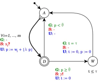
Figure 3.1: “Asynchronous neuron” model. Please note the graph represents a Timed Au-tomaton, it does not represent a Neural Network. The initial state is Accumulate, Decide is a committed state while Wait is a normal state subject to the t 6 τ . The (A → D) edge is actually a parametric and synthetic way to represent m edges, one for each input synapsis.

so it is possible to consider the leak factor as a constant instead of a decreasing function of time, leading to the following refined definition:

Definition 3.2. Let m ∈ N, then an Asynchronous Neuron NA is a tuple

(w, λ, θ, τ ), where:

• w = (w1, . . . , wm) ∈ {−R, . . . , R}m is the m-uple of weights,

• λ ∈ Q ∩ [0, 1] is the leak factor, • θ ∈ N is the threshold,

• τ ∈ N+ _{is the refractory period.}

The neuron behavior is then described by the Timed Automaton in Figure

3.1 and depends on the following channels, variables and clocks:

• x = (x1, . . . , xi, . . . , xm) is the m-uple of broadcast channels used to

receive input spikes,

• y is the output broadcast channel used to emit the output spike, • p ∈ N is an integer variable holding the current potential value, which

(27)

• t ∈ N is a clock, initially set to 0.

The automaton has three locations: A, D and W, which respectively stand for Accumulate, Decide and Wait. It can move from one location to another according following rules:

• it keeps waiting in location A for input spikes and whenever it receives a spike on input xi (i.e. it receives on channel xi) it moves to location

D updating p as follows:

p := wi+ bλ · pc

• while the neuron is in location D then time does not progress (since it is committed ); from this location, the neuron moves back to A if p < θ, or it moves to W, firing an output spike (i.e. writing on y) and resetting t, otherwise;

• the neuron will remain in location W for an amount of time equal to τ and then it will move back to location A resetting both p and t. Remark. The assumptions this model relies on are maybe too strong: it does not handle properly scenarios having input spikes occurrence times with non-negligible variance and it is expected to behave poorly in such cases. Basically, if no input spike occurs, time flow has no effect on the neuron, which is far from truth.

Implementation through Uppaal. A neural network with asynchronous neurons is implemented as an Uppaal system having global definitions shown in Listing 3.1. Each neuron is realized as a Template having the following parameters list:

// One b r o a d c a s t c h a n & xi for e a c h i n p u t

b r o a d c a s t c h a n & x1 , ... , w e i g h t _ t & w [ M_ < name >] , b r o a d c a s t c h a n & y

and declarations shown in Listing 3.2. Procedure input(i) is executed on each (A → D) edge firing, while reset() is executed on each firing of edge (W → A).

(28)

1 c l o c k t = 0; 2

3 int tau = <int>; 4 int t h e t a = <int>; 5 r a t i o _ t l a m b d a = { <int> , <int> }; 6 7 int p = 0; 8 9 v o i d i n p u t (int i ) { 10 p = ( w [ i ] * l a m b d a . den + l a m b d a . num * p o t e n t i a l ) / l a m b d a . den ; 11 } 12 13 v o i d r e s e t () { 14 p = 0; 15 }

Listing 3.2: Asynchronous neuron template declarations in Uppaal

Finally, it may be noticed that a minimal automaton can be obtained collapsing locations A and D. The reasons they have been kept separated are: (a) within some model-checking query, the presence of location D allows to express concepts like “the neuron has received a spike” or “the neuron is going to emit”; (b) when actually implementing the neuron in Uppaal, the presence of location D allows to reduce the number of required edges: without D we would have needed m loops on location A and m edges from A to W, so 2m + 1 total edges, considering the one from W to A; while thanks to D we only need m + 3 edges.

3.1.2 (Partially) Synchronous Model

We present here a second approach aimed at overcoming the limitations of the asynchronous model introduced above: it handles input spike co-occurrence, and time-dependent potential decay, even if no spike is received. The neuron is conceived as a synchronous and stateful machine that: (i) accumulates po-tential whenever it receives input spikes within a given accumulation period, (ii) if the accumulated potential is greater than the threshold, the neuron

(29)

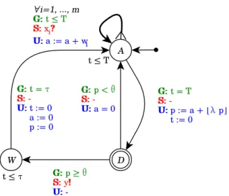
Figure 3.2: “Synchronous neuron” model. The (A → A) loop is actually a parametric and synthetic way to represent m edges, one for each input synapsis.

emits an output spike, (iii) it waits for refractory period, (iv) and resets to initial state. We assume that no two input spikes on the same synapse can be received within the same accumulation period (i.e., the accumulation period is shorter than the minimum refractory period of the input neurons).

Definition 3.3 (Synchronous Neuron). Let m ∈ N, then a Synchronous Neuron NS is a tuple (w, T, λ, θ, τ ), where:

• w = (w1, . . . , wm) ∈ {−R, . . . , R}m is the m-uple of weights,

• λ ∈ Q ∩ [0, 1] is the leak factor, • θ ∈ N is the threshold,

• τ ∈ N+ _{is the refractory period,}

• T ∈ N+ _{is the accumulation period.}

The neuron behavior, described by the Timed Automaton shown in Figure

3.2, depends on the following channels, variables and clocks:

• t, x, y and p are, respectively, a clock, the m-uple of input broad-cast channels, the output broadbroad-cast channel and the current potential variable, as for the asynchronous model,

(30)

• a ∈ N is a variable holding the weighted sum of input spikes occurred within the current accumulation period; it is 0 at the beginning of each period.

Locations are named as in the asynchronous model, but this one is subjected to different rules:

• the neuron keeps waiting in state A for input spikes while t 6 T and whenever it receives a spike on input xi it updates a as follows:

a := a + wi

• when t = T the neuron moves to state D, resetting t and updating p as follows:

p := a + bλ · pc

• since state D is committed, it does not allow time to progress, so, from this state, the neuron can move back to A resetting a if p < θ, or it can move to W, firing an output spike, otherwise;

• the neuron will remain in state W for τ time units and then it will move back to state A resetting a, p and t.

The innovation here is the concept of accumulation period. According to the asynchronous model, two inputs cannot occur into the same instant and, above all, their relative order is the only thing that influences the neuron po-tential: two consecutive input spikes would have the same effect regardless of their time difference. Thanks to the accumulation period of the synchronous model, the time distance between two consecutive spikes can be valorized: since the (A → D) edge firing, namely “the end of the accumulation period”, is not governed by input spikes as in the asynchronous model but only by time, the neuron potential will actually decay as time progress if no input is received.

Note that, if the assumption requiring one input not to emit more than once within the same accumulation period does not hold (i.e. inputs frequen-cies are too high), the neuron potential would increase as if the two spikes were from different synapses.

(31)

1 c o n s t int T = <int>;

2 c l o c k t = 0 . 0 ;

3 c o n s t int tau = <int>;

4 c o n s t int t h e t a = <int>; 5 r a t i o _ t l a m b d a = { <int> , <int> }; 6 7 int a = 0; 8 int p = 0; 9 10 v o i d r e s e t () { 11 a = 0; 12 p = 0; 13 } 14 15 v o i d i n p u t (int i ) { 16 a += w [ i ]; 17 } 18 19 v o i d e n d A c c u m u l a t i o n () {

20 p = ( a * l a m b d a . den + p * l a m b d a . num ) / l a m b d a . den ; 21 }

(32)

Implementation through Uppaal. A neural network with synchronous neurons is implemented as an Uppaal system having global definitions shown in Listing 3.1. It differs from the asynchronous model implementation only for the declarations, as shown in Listing3.3. Procedure input(i) is executed on each (A → A) loop firing, endAccumulation() is invoked on (A → D), while reset() is executed on each firing of edge (W → A). As for the asynchronous model, a minimal automaton can be obtained by removing state D and adding more edges.

3.2 Spiking neural networks as Timed

Au-tomata Networks

After showing how a Timed Automaton can represent a neuron, the main concern is about neuron interconnection, i.e., representing a Neural Network as a Timed Automata Network by means of some proper channel sharing convention. Another relevant matter covered by this section is about inputs and outputs representation, analysis and governance.

In order to make our models easier to inspect, we defined a language for input sequences specification. Here we show how to translate any word from such a language into a Timed Automaton able to emit it. Then we introduce non-deterministic input generators which are useful in those contexts where neurons must handle generic input sequences. Finally, we show how output consumers can be used to measure a neuron spike frequency.

Synapses connecting neurons are represented by automata sharing chan-nels. More formally, let I1, I2, . . . be input generators, let N , N1, N2, . . .

be neurons, and let O be an output consumer; then synapses are Timed Automata Networks obtained by parallel composition as follows:

• input generators to neuron: (I1, . . . , In) x

k N , where x = (x1, . . . , xn)

and each xi is a channel shared by Ii and N , carrying input spikes from

the former to the latter;

• neurons to neuron: (N1, . . . , Nn) y

k N , where y = (y1, . . . , yn) and

(33)

are received by N ;

• neuron to output consumer: N

y

k O, where y is a shared channel carrying N outputs which are consumed by O.

3.2.1 Input generators

Regular input generators. Essentially, input sequences are sequences of spikes and pauses: spikes are instantaneous while pauses have a non-null duration. Sequences can be empty, finite of infinite. After each spike there must be a pause except when the spike is the last event of a finite sequence, i.e., there exists no sequence having two consecutive spikes. Infinite sequences are composed by two parts: a finite and arbitrary prologue and an infinite and periodic part whose period is composed by a finite sequence of spike–pause couples.

Definition 3.4 (Input Sequence Grammar). Let s, p, ] and [ be terminal symbols, let I, N , P1, . . . , Pn and P be non-terminals and let x1, . . . , xn∈

N+ be some durations for a given n > 0, then:

I ::= ε | P ? (s P )∗(s ε | ((s P1) · · · (s Pn))ω) P ::= p[N ] p1 ::= p[x1] .. . Pn ::= p[xn]

represents the ω-regular expression for valid input sequences. In Definition3.4:

• s is a symbol representing a spike; • p is a symbol representing a pause;

• according to the productions of P and Pi, each pause is associated to

a natural-valued duration;

• p[N ] represents a pause whose duration is some number matching N , the regular expression for natural numbers;

(34)

• p[xi] represents a pause whose duration is a given number xi.

Notice that any pause within any valid input sequence is followed by a spike. We denote with Φ the finite prefix of an input sequence and with Ω the part which is repeated infinitely often, while α ranges over sub-sequences.

It is possible to generate an emitter automaton for any valid input se-quence. Such an automaton requires a clock t to measure pauses durations, a boolean variable s which is true every time the automaton is firing and a location for each spike or pause into the sequence. The encoding _{J I K of a} sequence I = ε | Φ | Φ Ωω is as follows:

• _{J ε K =} an empty sequence is encoded into an automaton having just one location E without any edge;

• _{J Φ K =} any finite sequence is encoded into a

sequence of locations, as described below, where the last one has no outgoing edges and represent the end of the sequence;

• _{J Φ Ω}ω

K = any infinite sequence is

composed by a finite sub-sequence Φ followed by a finite sub-sequence Ω repeated an infinite amount of times. The two sub-sequences are encoded according to the rules explained below and the resulting au-tomata are connected. Finally, an urgent location R is added, having an input edge from Ω last location and an output edge to Ω first loca-tion.

Any finite sub-sequence is a list of spikes and pauses. They are recursively encoded as follows:

• _{J p[N ] α K =} any pause having duration N and

followed by a sub-sequence α is encoded into a location P with the invariant t 6 T having one outgoing edge connected to the automaton J α K; such an edge is enabled if and only if t = T and, if triggered, t is

(35)

reset and, since pauses are always followed by spikes, the s variable is set to true;

• _{J s α K =} any spike followed by a sub-sequence α is

translated to an urgent location S having one output edge connected to the automaton translated from α; such an edge emits on y if triggered and resets s.

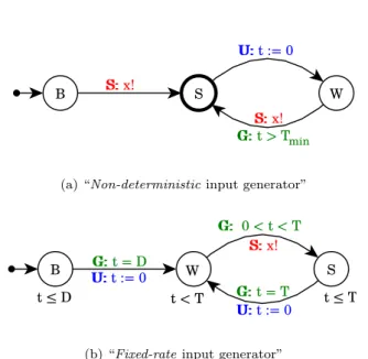
Non-deterministic input generators. If no assumptions are available or desirable about some neuron inputs, one can exploit non-deterministic input generators, i.e., automata able to fire randomly and only constrained to wait an amount of time Tmin between an emission and its successor. An

automaton of this sort is shown in Figure 3.3a and behaves as follows: • it waits in location B an arbitrary amount of time before moving to

location S, firing its first spike over channel x,

• since location S is urgent, the automaton instantaneously moves to location W, resetting clock t,

• from location W, after an arbitrary amount of time t ∈ ] Tmin, ∞ [, it

moves to location S, firing a spike.

Remark. One may introduce an initial delay D by adding invariant t ≤ D to location B and guard t = D on edge (B → S)

Fixed-rate input generators. Some contexts may consider input se-quences having fixed rates, i.e., the expected amount of spikes during some given time window T is constant, even if the sequence is not formally peri-odic since the distribution of spikes within two different time windows may differ. We propose the automaton shown in Figure 3.3b, which is able to non-deterministically produce an output spike for each discrete time window T , after it has been quiescent for an initial delay D:

• it waits in location B until clock t value equals to D, then it moves to location W, resetting it;

(36)

(a) “Non-deterministic input generator”

(b) “Fixed-rate input generator”

Figure 3.3: Automata generating input sequences. Non-deterministic generators are only con-strained to wait more than Tmintime units between emissions. Fixed-rate generators are only

constrained to fire exactly once for each period T .

Figure 3.4: “Output consumer” automaton. Its initial location is Wait, location Output is urgent, since-last-spike is a clock while even is a boolean variable.

• it waits in location W a non-deterministic amount of time ts∈ ] 0, T [

and then it moves to location S firing a spike over channel x; • finally, it waits T − ts time units in S before moving back to W.

3.2.2 Output consumers

As shown in Section3.1, neuron models emit outputs writing on some broad-cast channel y. In order to query a model-checker about output neurons out-comes, the output consumer automaton shown in Figure 3.4 is connected to each neuron by sharing its output channel. Its behavior is straightforward:

(37)

• it waits in location W for the neuron it is connected to to emit an output spike, which makes it move to location O;

• since location O is urgent, the automaton will instantly move back to location W resetting s and setting e to its negation;

where s is the clock measuring the elapsed time since last emission and e is a boolean variable which differentiates each emission from its successor.

So if an output consumer automaton is in location O then its correspond-ing neuron has just emitted one spike.

(38)

Chapter 4 Validation of the Leaky

Integrate & Fire model

In this chapter we validate the synchronous neuron model against its ability of reproducing some behaviors, as described by Izhikevich in [14].

First we recall the following concepts:

Definition 4.1 (Input (sub-)sequence). Let I1, . . . , Im be a input sources

(i.e., neuron or generators) connected to some neuron N , and let Fi =

{ti,1, ti,2, . . .} be the ordered set of firing times of Ii; then I =

Sm i=1Fi is

the ordered input sequence of N . For any continuous interval Q ⊂ R+0 the

set I ∩ Q is a sub-sequence of I.

Definition 4.2 (Output (sub-)sequence). Let N be a neuron and let FN =

{t1, t2, . . .} be its ordered set of firing times; then FN is the ordered output

sequence of N . For any continuous interval Q ⊂ R+0 the set FN ∩ Q is a

sub-sequence of FN.

Definition 4.3 (Persistent input (sub-)sequence). Let N = (w, T, λ, θ, τ ) be a Synchronous Neuron, let I be its input (sub-)sequence and let t range over the accumulation periods starting instants; then I is persistent if and only if card(I ∩ [ t, t + T [) > 0, ∀t.

Definition 4.4 (Persistent excitatory/inhibitory input (sub-)sequence). Let N = (w, T, λ, θ, τ ) be a Synchronous Neuron, let I be its input sub-sequence and let n range over the accumulation periods; then I is excitatory (resp.

(39)

inhibitory) if and only if An > 0 (resp. An < 0) ∀t, where An is the sum of

weighted inputs for the n-th accumulation period.

Definition 4.5 (Persistent constant input (sub-)sequence). Let N = (w, T, λ, θ, τ ) be a Synchronous Neuron, let I be its input sub-sequence and let n range

over the accumulation periods; then I is constant if and only if there exists some K ∈ Z such that An = K, ∀t.

Definition 4.6 (Periodic output (sub-)sequence). Let N be a neuron and let FN = {t1, t2, . . .} be its output sequence, then FN is periodic if and only

if there exists some P ∈ R+ such that ti+1− ti = P, ∀i.

Definition 4.7 (Simultaneous input spikes). Let N = (w, T, λ, θ, τ ) be a Synchronous Neuron, let I be its input sequence, let t range over the accumulation periods starting instants and let s1, s2 ∈ I be two input spikes;

then s1 and s2 are simultaneous if and only if s1, s2 ∈ [ t, t + T [ for some t.

Definition 4.8 (Consecutive input spikes). Let N = (w, T, λ, θ, τ ) be a Synchronous Neuron, let I be its input sequence, let t, t0 be the starting instants of some accumulation period and the next one, respectively, and let s1, s2 ∈ I be two input spikes; then s1 and s2 are consecutive if and only if

s1 ∈ [ t, t + T [∧s2 ∈ [ t0, t0+ T [.

Definition 4.9 (Reset times). Let N be a neuron and let FN = {t1, t2, . . .}

be its output sequence, then the set of reset times of N is ZN = {t + τ : t ∈

FN}.

We use calligraphic letters (A) for automata, bold letters (X) for au-tomata states, and lower-case italic letters (t) for auau-tomata variables or clocks. Within temporal logic formulae, the predicate stateA(X) is 1 if and

only if automaton A is in state X, 0 otherwise, and evalA(t) is a function

mapping a variable or clock t to the value it currently carries within the context of automaton A: a predicate may consist of the comparison between such a value and a constant. For boolean variables we may abuse the nota-tion writing eval(b) and ¬evalA(b) instead of evalA(b) = 1 or evalA(b) = 0,

(40)

4.1 Intrinsic Properties

Maximum threshold. Here we show that, assuming an upper bound for the sum of ingoing synapses weights, there exist a way to compute the max-imum threshold value such that, any neuron having a threshold greater than or equals to it, will never be able to fire.

Property 4.1 (Threshold-leak factor relation). Let N = (w, T, λ, θ, τ ) be a Synchronous Neuron and amax∈ N+the maximum value of weighted inputs

sum, then, if θ ≥ amax

1−λ, the neuron is not able to fire.

Proof. Without loss of generality, we suppose that, during each accumulation period, N receives the maximum possible input amax. Then, its potential

function is:

pn = amax+ bλ · pn−1c

which is always lower than or equal to its undiscretized version: pn≤ p0n = amax+ λ · p0n−1

The same inequality can be written in explicit form because of Equation 2.3:

pn ≤ p0n= n

X

k=0

an−k· λk

and, since we assumed the neuron always receives amax, an−k is constant and

do not depend on k: pn≤ amax· n X k=0 λk

The rightmost factor is a geometric series having a more compact represen-tation:

pn ≤ amax·

1 − λn

1 − λ

which reaches its maximum value _1−λ1 for n → ∞, therefore:

pn ≤

amax

1 − λ, ∀n ∈ N Thus, if θ ≥ amax

1−λ, it is impossible for the neuron potential to reach the

(41)

Notice that, according to Definition3.3, synapses weights are never greater than an integer R, so amax = mR for each neuron having m ingoing synapses,

even if, in the general case, we will consider amax =

Pm

i=0wi ≤ mR. We will

say that a neuron is firing enabled if θ < amax

1−λ.

Analysis of neuron timings. We can quantify the amount of time that the neuron requires to complete an accumulate–fire–rest cycle. Such expres-sion is useful to prove some interesting properties, e.g., here we show that there exists a minimum delay between one neuron emission and its successor. Property 4.2 (Minimum firing period). Let N = (w, T, λ, θ, τ ) be a firing enabled Synchronous Neuron, then the time difference between successive firings cannot be lower than T + τ .

Proof. Let An = PT_k=1ak+t0 be the sum of weighted inputs during the n-th

accumulation period, then the neuron behavior can be described as follows:

pn = An+ bλ · pn−1c (4.1)

is the potential value after the n-th accumulation period. If the neuron will eventually fire an output spike, then there exists ˆn > 0 such that:

ˆ

n = arg min

n∈N

{pn: pn≥ θ} (4.2)

i.e., the firing will occur at the end of the ˆn-th accumulation period, which means during the ˆt-th time unit since t0, thus:

ˆ

t = ˆn · T + t0 (4.3)

where t0 is the last reset time, i.e., the last instant back in time when the

neuron completed its refractory period. Then the next reset time t0, i.e., the next instant in future when the neuron will complete its refractory period, after having emitted a spike, is:

t0 = ˆt + τ = ˆn · T + τ + t0

At instant t0, the neuron quits its refractory period, n is reset to 0, t0 is set

(42)

Such a way to describe our model dynamics allow us to express the inter-firing period as a function of ˆn:

t0− t0 = ˆn · T + τ (4.4)

So, the minimum inter-firing period is T + τ for ˆn = 1. Such a property can be verified as follows: let I be the non-deterministic input generator having Tmin = 1 and, without loss of generality1, initial delay D = T + τ , then the

Timed Automata Network I

x

k N

y

k O satisfies the following formula:

AG(stateO(O) =⇒ evalO(s) ≥ T + τ ) (4.5)

where s measures the time elapsed since last firing, meaning that, whenever the output consumer receives a spike, the time elapsed since the previous received spike cannot be lower than T + τ .

Analysis of neuron memory. Here we discuss about the neuron capa-bility of taking past events into account when computing its outcome. As argued above, the neuron potential is affected by every input spike it received since the last reset time, but every event that occurred before that instant is forgotten.

Definition 4.10 (Neuron inter-emission memory). Let N be a neuron, let ZN be its reset times set and let I be an input sub-sequence; then N has

inter-emission memory if and only if there exist two different t, t0 ∈ ZN such

that the output sub-sequence produced by N as a response to I starting from t differs from the output sub-sequence it produces as a response to I starting from t0.

Property 4.3 (Memoryless neuron). Let N = (w, T, λ, θ, τ ) be a Syn-chronous Neuron, then N has not inter-emission memory.

Proof. According to Definition3.3 each reset time occurs on each (W → A) firing. Such event makes N automaton move back to its initial location while resetting clock t and variables p and a, making them equal to their starting values. So it is impossible for the neuron to behave differently if subjected to the same input sub-sequence.

1_{the initial delay is required in order to make the formula hold for the first output spike}

(43)

Analysis of inhibitory inputs. Here we argue about the effects of an inhibitory stimulation to a neuron whose potential lower than its threshold. Property 4.4 (Inhibitory effect of negative stimulations). Let N = (w, T, λ, θ, τ ) be a Synchronous Neuron, let Anbe the sum of weighted inputs received

dur-ing the current accumulation period and let pn−1 be the neuron potential at

the end of the previous accumulation period, then if pn−1 < θ and An < 0

the neuron cannot fire at the end of the current accumulation period. Proof. It is sufficient to prove that, under such hypotheses, pn< θ.

Consid-ering pn definition, we can state that:

pn≤ An+ λ · pn−1

so, since An is negative, we can rewrite it as −|An|:

pn+ |An| ≤ λ · pn−1

and then we deduce:

pn< λ · pn−1

because pn < pn+ |An| and, consequently:

pn ≤

1

λ · pn < pn−1 because λ−1∈ [ 1, ∞ [. So finally:

pn < pn−1 < θ

Next we show that only positive stimulations are necessary for the neuron to produce emissions:

Property 4.5. Let N = (w, T, λ, θ, τ ) be a Synchronous Neuron such that θ > 0, let An be the sum of weighted inputs received during the current

accumulation period and let pn be the neuron potential at the end of the

(44)

Figure 4.1: Tonic spiking representation for continuous signals from [14].

Proof. It is sufficient to prove that, under such hypotheses, An > 0. We

know that:

pn= An+ bλ · pn−1c ≥ θ

Let’s analyze two sub-cases, with respect to the sign of bλ · pn−1c − θ:

Consider the case: bλ · pn−1c < θ.

According to the initial hypothesis: bλ · pn−1c < θ ≤ An+ bλ · pn−1c

and, consequently:

0 < θ − bλ · pn−1c ≤ An

so, finally An > 0.

Consider the case: bλ · pn−1c ≥ θ.

This means pn−1 ≥ θ, in fact:

pn−1 ≥ λ · pn−1 ≥ bλ · pn−1c ≥ θ

But this is absurd because if pn−1≥

θ, the neuron emits and resets, thus its potential in the next accumula-tion period is zero, which is in con-tradiction with the hypothesis pn≥

θ > 0.

4.2 Capabilities

Tonic Spiking. “Tonic spiking” is the behavior of a neuron producing a periodic output sub-sequence as a response to a persistent excitatory constant input sub-sequence. An example is shown in Figure 4.1.

Property 4.6 (Tonic spiking). Let N = (w, T, λ, θ, τ ) be a Synchronous Neuron having only one ingoing excitatory synapse such that w > 0 and

(45)

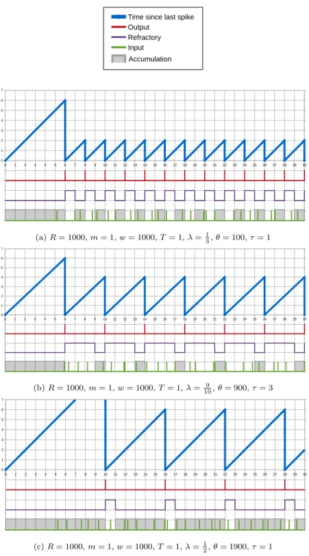
(a) R = 1000, m = 1, w = 1000, T = 1, λ =1

3, θ = 100, τ = 1

(b) R = 1000, m = 1, w = 1000, T = 1, λ =₁₀9, θ = 900, τ = 3

(c) R = 1000, m = 1, w = 1000, T = 1, λ = 1

2, θ = 1900, τ = 1

Figure 4.2: Tonic spiking simulations. Each diagram shows the time elapsed since last neuron emission (blue), the emitted spikes (red), the refractory periods (purple) and input spikes (green) within accumulation periods (gray) for three different neurons and for 30 time units. In each case, the input generator is a fixed-rate generator having initial delay 5 and time window size 1.

(46)

θ < w/(1 − λ) and let I be the input source connected to N producing a persistent input sequence, then N produces a periodic output sequence. Proof (Sketch). Let I be the fixed-rate input generator having arbitrary ini-tial delay D and time window size T , and let O be an output consumer, then the Timed Automata Network I

x

k N

y

k O satisfies the following formulae: 





stateO(O) ∧ evalO(e) stateO(O) ∧ ¬evalO(e)

stateO(O) ∧ ¬evalO(e) stateO(O) ∧ evalO(e)

(4.6)

where O is the location that automaton O reaches after consuming a spike and e is boolean variable whose value changes whenever O moves into location O. So, whenever automaton O reaches location O it will eventually reach it again. As shown in Figure 4.2, if we simulate neurons having different parameters providing them the same input I, then they keep producing a periodic outcome whose period only depends on T and τ as long as θ <

w 1−λ.

It should be noted that one may also find the value P of the period of some given neuron N by means of simulations, thus the periodic behavior can be proven by a model-checker verifying the following formula:

AG(stateO(O) ∧ evalN(f ) =⇒ evalO(s) = P ) (4.7)

where s is the clock measuring the time elapsed since last spike consumed by O, and f is a boolean variable of automaton N which is initially f alse and is set to true when edge (W → A) fires (i.e., it indicates whether N has already emitted the first spike and waited the first refractory period or not). Integrator. “Integrator” is the behavior of a neuron producing an output spike whenever it receives at least a specific number of simultaneous spikes from different input sources or when it receives a certain amount of consec-utive spikes from a specific input source. So the neuron parameters can be tuned in order to detect (i.e., fire as a consequence of) a given number of simultaneous or consecutive spikes. An example is shown in Figure 4.3.

(47)

Figure 4.3: Integrator behavior representation for continuous signals, from [14].

Property 4.7 (Simultaneous integrator). Let N = ((R, . . . , R), T, λ, n, τ ) be a Synchronous Neuron having m synapses with maximum excitatory weight R and an integer threshold n ≤ m, then the neuron emits if it receives a spike from at least n input sources during the same accumulation period.

Proof (Sketch). Let I1, . . . , Im be non-deterministic input generators

con-strained to wait more than T time units between an emission and its succes-sor, and let O be an output consumer, then the Timed Automata Network (I1, . . . , Im)

x

k N

y

k O satisfies the following formula stating that, if at least n generators are in location S while N is in A, then O will eventually capture an output of N : m X i=1 statei(S) ≥ n !

∧ stateN(A) stateO(O) (4.8)

where S is the location that each automaton Ii reaches after producing a

spike and A is the accumulation location of the neuron N . As shown in Figure 4.4a, a neuron, under such hypotheses, will fire as soon as it receive n simultaneous spikes.

Notice that, since potential depends on past inputs too, the neuron may still be able to fire in other circumstances, e.g., if it keeps receiving less than n spikes for a sufficient number of accumulation periods, then it may eventually fire.

(48)

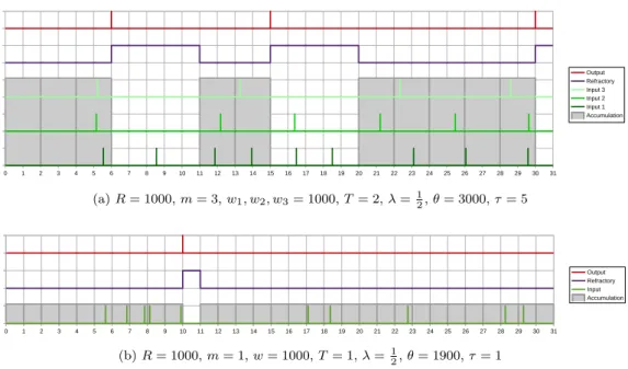
(a) R = 1000, m = 3, w1, w2, w3= 1000, T = 2, λ =1₂, θ = 3000, τ = 5

(b) R = 1000, m = 1, w = 1000, T = 1, λ =1₂, θ = 1900, τ = 1

Figure 4.4: Chart4.4arepresents the behavior of a neuron, having 3 ingoing synapses, which is able to detect the simultaneity of at least 3 inputs: whenever two or more input spikes (green lines) occur during the same accumulation period (gray), an output spike is produced (red). Chart4.4brepresents the behavior of a neuron, having a single ingoing synapse, which is able to detect a sequence of 5 consecutive input spikes.

Property 4.8 (Sequential integrator). Let N = (w, T, λ, θ, τ ), be a Syn-chronous Neuron having only one ingoing synapse, such that θ < _1−λw , then there exists a maximal sequence of consecutive input spikes of length ˆn that results in an output spike.

Proof (Sketch). Let I be the fixed-rate input generator having arbitrary ini-tial delay D and time window size T , let O be an output consumer, and let ˆn be the minimum amount of consecutive input spikes required to make the potential overcome the threshold, obtained by means of simulation or by recursively computing pnuntil it reaches the threshold value; then the Timed

Automata Network I

x

k N

y

k O satisfies the following formula stating that, whenever O receives a spike, the number of consecutive spikes never greater than ˆn:

AG(stateO(O) =⇒ evalN(c) ≤ ˆn) (4.9)

where c is an integer variable of automaton N counting the amount of con-secutive accumulation periods that received at least one spike since last emis-sion.