HAL Id: tel-00499281
https://tel.archives-ouvertes.fr/tel-00499281
Submitted on 9 Jul 2010
HAL is a multi-disciplinary open access archive for the deposit and dissemination of sci-entific research documents, whether they are pub-lished or not. The documents may come from teaching and research institutions in France or abroad, or from public or private research centers.
L’archive ouverte pluridisciplinaire HAL, est destinée au dépôt et à la diffusion de documents scientifiques de niveau recherche, publiés ou non, émanant des établissements d’enseignement et de recherche français ou étrangers, des laboratoires publics ou privés.
Benoît Cerutti
To cite this version:
Benoît Cerutti. High-energy gamma-ray emission in compact binaries. Astrophysics [astro-ph]. Uni-versité de Grenoble, 2010. English. �tel-00499281�
THÈSE
présentée parBenoît C
ERUTTIpour obtenir le diplôme de Docteur en sciences de l’Université de Grenoble (Arrêté ministériel du 7 août 2006)
Spécialité : ASTROPHYSIQUE & MILIEUX DILUÉS
High-energy gamma-ray emission in compact binaries
-Emission gamma de haute énergie dans les systèmes
binaires compacts
Dirigée par
Guillaume DUBUS & Gilles HENRI
Soutenue publiquement le 10 juin 2010 devant le jury composé de
M. Frédéric DAIGNE Rapporteur M. Guillaume DUBUS Examinateur Mme Isabelle GRENIER Examinateur M. Gilles HENRI Examinateur
M. John KIRK Rapporteur
M. Julien MALZAC Examinateur M. François MONTANET Président
Thèse préparée au sein de l’Équipe
Laboratoire d’Astrophysique de Grenoble
High-energy gamma-ray emission in compact
binaries
-Emission gamma de haute énergie dans les
systèmes binaires compacts
PhD thesis — Université de Grenoble
Je voudrais commencer par remercier sincèrement Guillaume Dubus avec qui j’ai vécu trois années passionnantes et très stimulantes. Ce fut un réel plaisir et une chance de travailler avec Guillaume. Merci à Gilles Henri pour sa gentillesse et ses conseils avisés, en particulier sur les aspects les plus théoriques de ma thèse. J’ai également eu la chance de collaborer avec Julien Malzac avec qui j’ai également beaucoup appris. Je souhaiterai remercier les deux rapporteurs de ma thèse, John Kirk et Frédéric Daigne qui ont accepté cette tâche malgré les courts délais imposés et la longueur du manuscrit. J’ai beaucoup apprécié de travailler et de discuter avec Adam Hill et Anna Szostek. Merci à Anna pour son aide et ses commentaires sur le manuscrit de thèse. L’accueil très chaleureux de l’équipe Sherpas et de l’ensemble du laboratoire a aussi grandement contribué à mon bien-être au cours de cette thèse. J’en profite d’ailleurs pour remercier l’ensemble des thésards que j’ai connu au laboratoire, en particulier Timothé Boutelier et Astrid Lamberts avec qui j’ai partagé le même bureau. J’ai été également ravi de travailler avec Sarkis Rastikian. Merci à mes amis, qui sont venu parfois de loin (même de Suède!) pour assister à ma soutenance. Enfin, mes dernières pensées vont à mes parents et à mon frère qui m’ont toujours soutenu et qui ont toujours été présents.
Remerciements i
Table of contents ix
List of figures ix
List of tables xxi
Part 1. INTRODUCTION 1
CHAPTER 1. What is this thesis about? 3
1. The cosmic accelerators uncovered by the gamma-ray astronomy 3
2. Binary systems in the gamma-ray sky! 4
§ 1. Gamma-ray binaries 4
§ 2. Microquasars 6
3. Objectives of this thesis: What we want to understand 7
4. Guidelines: How is this thesis constructed? 8
[Français] De quoi parle cette thèse? 11
5. Les accélérateurs cosmiques découverts par l’astronomie gamma 11
6. Des systèmes binaires dans le ciel gamma! 11
§ 3. Les binaires gamma 12
§ 4. Microquasars 13
7. Objectifs de cette thèse: Ce que nous voulons comprendre 13
8. Comment cette thèse est-elle construite? 14
CHAPTER 2. Relevant high-energy processes 15
1. What we want to know 18
2. High-energy leptonic processes 18
§ 5. Inverse Compton scattering 18
§ 6. Bremsstrahlung 21
§ 7. Synchrotron radiation 23
§ 8. Triplet pair production 25
§ 9. Relevant leptonic processes in binaries 27
3. High-energy hadronic processes 28
§ 10. Proton-proton collision 29
§ 11. Photomeson production 31
4. Photon-photon annihilation 32
5. The cooling of relativistic particles 33
§ 12. The continuity equation 33
§ 13. General solution 34
§ 14. Some simple solutions 34
6. What we have learned 35
7. [Français] Résumé du chapitre 35
§ 15. Contexte et objectifs 35
§ 16. Ce que nous avons appris 36
Part 2. GAMMA-RAY EMISSION IN GAMMA-RAY BINARIES 37
CHAPTER 3. Anisotropic inverse Compton scattering 39
1. What we want to know 40
2. Kinematics and geometrical quantities 40
3. Differential cross sections 41
4. Anisotropic inverse Compton scattering in the Thomson approximation 42
§ 17. Soft photon density 42
§ 18. Anisotropic Thomson kernel 43
§ 19. Anisotropic scattering rate 44
§ 20. Beamed emission 45
§ 21. Isotropic Thomson kernel 45
§ 22. Integration over electron energy for a power law distribution 46
§ 23. Integration over soft photon energy for a black-body distribution 47 § 24. Final check: Integration over an isotropic distribution of soft radiation 49
5. Anisotropic inverse Compton scattering in the general case 50
§ 25. General anisotropic kernel 50
§ 26. Integration over a power law for electrons and a black body for soft photons 51
§ 27. Final check: Comparison with Jones’ isotropic solution 51
6. What we have learned 52
7. [Français] Résumé du chapitre 53
§ 28. Contexte et objectifs 53
§ 29. Ce que nous avons appris 54
CHAPTER 4. Gamma-ray modulation in gamma-ray binaries 55
1. What we want to know 56
2. The model 57
§ 30. The magnetic field 57
§ 31. The electron distribution 57
§ 32. Gamma-ray emission and pair production 59
3. Application to gamma-ray binaries 60
§ 33. LS 5039 60
§ 34. LS I +61 303 and PSR B1259-63 63
4. What we have learned 64
§ 35. Contexte et objectifs 67
§ 36. Ce que nous avons appris 68
6. Paper: The modulation of the gamma-ray emission from the binary LS 5039 69
CHAPTER5. High-energy emission from the unshocked pulsar wind 83
1. Direct emission from the pulsar wind in gamma-ray binaries? 84
2. What we want to know 85
3. Compton drag of the pulsar wind 85
§ 37. Assumptions and geometry 85
§ 38. Anisotropic inverse Compton cooling of pairs 86
§ 39. Calculation of the cooled Lorentz factor in binaries 87
§ 40. Lorentz factor profiles and maps in LS 5039 and LS I +61 303 90
§ 41. Finite-size star and thermal spectrum 91
4. Inverse Compton emission 92
§ 42. The density of pairs 92
§ 43. Inverse Compton spectrum 94
§ 44. Pair production 96
5. Size and geometry of the pulsar wind nebula 96
6. What if the pulsar wind is anisotropic? 98
§ 45. Anisotropic pulsar wind 98
§ 46. The pulsar orientation 99
§ 47. Lorentz factor maps 101
§ 48. What are the odds to observe a low Lorentz factor? 101
7. Free pulsar wind emission in LS 5039 and LS I +61 303 103 8. Signature of the unshocked wind seen by Fermi? 104
9. Striped pulsar wind 107
10. What we have learned 108
11. [Français] Résumé du chapitre 109
§ 49. Contexte et objectifs 109
§ 50. Ce que nous avons appris 110
12. Paper: Spectral signature of a free pular wind in the gamma-ray binaries LS 5039
and LS I +61 303 112
Part 3. PAIR CASCADE EMISSION IN GAMMA-RAY BINARIES 125
CHAPTER6. Anisotropic pair production 127
1. What we want to know 127
2. Kinematics and threshold energy 128
3. Cross sections 129
4. Construction of the center-of-mass frame 130
§ 51. Geometrical construction 130
§ 52. Lorentz transform parameters 131
6. The spectrum of the produced pair 132
§ 53. General solution 132
§ 54. Anisotropic pair production kernel 133
§ 55. Integration over a power-law energy distribution and anisotropic effects 134
§ 56. Comparison with the isotropic and mono-energetic solution 134
§ 57. Comparison with Böttcher & Schlickeiser solution 135
7. The density of pairs 136
8. What we have learned 138
9. [Français] Résumé du chapitre 138
§ 58. Contexte et objectifs 138
§ 59. Ce que nous avons appris 138
CHAPTER 7. One-dimensional pair cascading 141
1. What we want to know 142
2. Assumptions and approximations for 1D cascade 143
3. Equations for anisotropic 1D cascade 144
§ 60. Equation for photons 144
§ 61. Equation for pairs 145
§ 62. Numerical integration 147
4. The development of 1D pair cascade in binaries 147
5. Anisotropic effects 149
6. 1D cascade emission in LS 5039 149
7. The density of escaping pairs 151
8. Pair cascading in the free pulsar wind 152
9. What we have learned 154
10. [Français] Résumé du chapitre 154
§ 63. Contexte et objectifs 154
§ 64. Ce que nous avons appris 155
11. Paper: One dimensional pair cascade emission in gamma-ray binaries 157
CHAPTER 8. Three-dimensional pair cascading 169
1. Assumptions on the ambient magnetic field 170
2. The first generation of pairs in binaries 171
§ 65. Spectrum and energy of pairs 172
§ 66. Absorption and spatial distribution of pairs 173
3. The first generation of gamma rays in binaries 174
§ 67. Geometry 174
§ 68. Equations for the first generation of gamma rays in the cascade 175
§ 69. Anisotropic effects 178
§ 70. Spatial distribution in LS 5039 179
4. Beyond the first generation approximation 180
§ 71. Semi-analytical approach 180
§ 73. The effect of the magnetic field 183
5. 3D pair cascade emission in LS 5039 184
§ 74. Modulation and spectra 185
§ 75. The location of the TeV source 185
§ 76. The ambient magnetic field in LS 5039 187
6. What we have learned 187
7. [Français] Résumé du chapitre 189
§ 77. Contexte et objectifs 189
§ 78. Ce que nous avons appris 191
8. Paper: Modeling the three-dimensional pair cascade in binaries 193
Part 4. HIGH-ENERGY EMISSION FROM RELATIVISTIC OUTFLOW 205
CHAPTER9. Anisotropic Doppler-boosted emission 207
1. What we want to know 207
2. Geometry and assumptions 208
3. Boosted synchrotron radiation 209
4. Boosted anisotropic inverse Compton scattering 210
§ 79. Soft photon density in the comoving frame 211
§ 80. Doppler-boosted Compton spectrum 212
5. What we have learned 214
6. [Français] Résumé du chapitre 215
§ 81. Contexte et objectifs 215
§ 82. Ce que nous avons appris 215
CHAPTER10. Doppler-boosted emission in gamma-ray binaries 217
1. Observational backdrop 217
2. The model and the geometry 218
3. LS 5039 218
4. LS I +61 303 219
5. PSR B1259-63 221
6. What we have learned 221
7. [Français] Résumé du chapitre 223
§ 83. Contexte et objectifs 223
§ 84. Ce que nous avons appris 224
8. Paper: Relativistic Doppler-boosted emission in gamma-ray binaries 225
CHAPTER11. Doppler-boosted emission in the relativistic jet of Cygnus X−3 237
1. Observational backdrop 237
2. The model and the geometry 238
3. Results 240
4. Absorption and location of the gamma-ray source 240
§ 86. Gamma-ray absorption and application to Cygnus X-3 244
5. What we have learned 245
6. [Français] Résumé du chapitre 247
§ 87. Contexte et objectifs 247
§ 88. Ce que nous avons appris 248
7. Paper: The relativistic jet of Cygnus X-3 in gamma rays 249
Part 5. CONCLUSION 257
CHAPTER 12. Conclusion 259
1. What we have learned 259
§ 89. Gamma-ray emission in gamma-ray binaries 259
§ 90. Pair cascade emission in gamma-ray binaries 260
§ 91. High-energy emission from relativistic outflows 261
2. Open questions and looking forwards 262
[Français] Conclusion 265
3. Ce que nous avons appris 265
§ 92. L’émission gamma dans les binaires gamma 265
§ 93. Emission d’une cascade de paires dans les binaires gamma 266
§ 94. Emission de haute énergie dans les écoulement relativistes 267
4. Questions ouvertes et perspectives 268
Part 6. REFERENCES 271
1 Top view of the compact object orbit (blue line) in Cygnus X−3 (top left), LS 5039 (top right), LS I+61◦303 (bottom left) and PSR B1259−63 (bottom right). The red filled disk
represents the massive star at scale in the system and the back solid line indicates
periastron. The observer sees the orbit from the bottom. 5 2 This sketch depicts the main components in gamma-ray binaries involved in the
non-thermal emission mechanism, in the pulsar wind nebula scenario (see the text for
explanations). 7
3 Sketch of a microquasar and of its different components. Energetic particles are
accelerated in the relativistic jet and radiate high-energy emission. 8 4 Total cross section for inverse Compton scattering as a function of x = ǫ′0/mec2. The
dashed line separates the Thomson (x ≪ 1) to the Klein-Nishina regime (x ≫ 1). The approximate formula given in Eq. (5.3) is shown with a red dashed line. 19 5 Numerically integrated inverse Compton energy losses (Eq. 5.8, blue solid line) of an
electron of energy Ee = γemec2bathed in a isotropic gas of photons with a black body
energy distribution of effective temperature T⋆ = 40 000 K. The analytical formula in
the Thomson (red dashed line) and Klein-Nishina (red dashed-dotted line) regimes are
overplotted for comparison. 20
6 Variations of φ1(blue line) and φ2(red line) as a function of ∆ for the neutral hydrogen
atom. 22
7 Bremsstrahlung spectrum (plot of the function fbdefined in Eq. 6.13) emitted by one electron of Lorentz factor γe = 10 (bottom curve), 100, 1000, and= ∞(top curve) as a
function of the ratio ǫ1/γemec2. The medium is composed of neutral hydrogen atoms
only. 23
8 Variations of fsdefined in Eq. (7.23) as a function of ǫ1/ǫc. 24
9 Total triplet pair production cross section as a function of x. The blue line corresponds to the expression valid for x >16. The Bethe-Heitler formula ∆BH, valid for x> 104, is
shown by the red dashed line. The total inverse Compton cross section is also shown for
comparison (green solid line). 26
10 Triplet pair production energy losses as a function of x for θ0 = π/2 given in Eq. (8.39).
One should trust only the domain where x & 103, below the energy losses are
overestimated but the variations are still qualitatively correct. Inverse Compton losses
are shown for comparison (red dashed line). 27
11 Leptonic cooling timescales: inverse Compton (solid line, "Th." in the Thomson limit and "KN" in the Klein-Nishina regime), synchrotron (dotted line, "Syn."), TPP (dashed line),
and Bremsstrahlung (dot-dashed line, "Brem."), as a function of the electron Lorentz factor γe. This plot shows also the total cooling timescale ttot(red dashed line) defined as
ttot−1 = t−1ic +tsyn−1 +t−1TPP+t−1B . The parameters used here are compatible with LS 5039: T⋆ = 39 000 K, R⋆ = 9.3R⊙, v∞ = 2400 km s−1, ˙M =10−7M⊙yr−1and d ≈0.1 AU at
periastron. The magnetic field is unknown but is chosen here as B=1 G. 29 12 Inclusive cross section of the production of neutral pions in proton-proton collision σpp,
as a function of the high-energy proton energy Ep. 30
13 Total cross section for pair production σγγas a function of β (left panel) and as a function
of the gamma-ray photon energy ǫ1 (right panel) for ǫ0 = 1 eV and θ0 = π. The pair is
mostly produced close to threshold (maximum for β ≈0.7). 32 14 Inverse Compton scattering seen in the observer frame (left panel) and in the rest frame
of the electron (right panel). Waves represent photons and the green thick arrow shows the direction of motion of the electron of total energy Ee = γemec2. The Lorentz boost
from the observer to the rest frame of the electron is along the z-axis. 41 15 Second order Feynman diagram for Compton scattering. 42 16 Geometrical configuration for the computation of the anisotropic inverse Compton
kernel. 42
17 Variations of the functions fanis(x)(red line) and fiso(x)(blue line) that appear in the
computation of the Compton kernel in the Thomson approximation. 46 18 Comparison of the analytical solution (red dashed line) to the numerically integrated
solution (blue solid line) for electrons with a power energy distribution and mono-energetic soft photons. Parameters used: ǫ0 = 10 eV, θ0 = π, p = 2. The effect of the
low and high energy cut-off are shown on the numerical solution where γ− =102 and
γ+=104. 47
19 The same as in Fig. 18, but where the kernel is integrated over a black-body energy distribution of effective temperature T⋆ =39000 K, with θ0 =180◦(top) , 120◦, 90◦, 60◦,
and 30◦(bottom). 48
20 Variation of the term responsible for the angular dependence in the Thomson spectrum
(1−µ0)p+1/2(see Eq. 23.124) as a function of µ0, with indices p=0.5, 1, 2 and 3. 49
21 The same as in Fig. 19, with γ−= 102and γ
+=107. θ0 =180◦ (top) , 120◦, 90◦, 60◦, and
30◦(bottom). 52
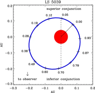
22 The same as in Fig. 21 if the gas of target photons is isotropic. The Compton emission is computed with the isotropic kernel of Jones (1968) (blue solid line) and comparison with the anisotropic solution averaged over all the angles (red dashed line). 53 23 Left panel: This diagram shows the orbit of the compact object (blue line) and the massive
companion star (red disk) in LS 5039 (top view). The distant observer is at bottom (indicated by the arrow). The orbital parameters are taken from Casares et al. (2005b). The orbital phases φ are given by the numbers where φ ≡ 0 at periastron. Superior conjunction corresponds to φ ≈ 0.06 and inferior conjunction to φ ≈ 0.72. Right panel: The angle ψ between the unit vector e⋆ and eobs varies between ψsup = π/2+iat
superior conjunction and ψin f =π/2−iat inferior conjunction, where i is the inclination
of the orbit. The green disk indicates the position of the compact object in the orbit. 56 24 Top panel: Steady-state cooled electron energy distribution for B =0.1 (top), 1 and 10 G
(bottom). The compact object injects electrons with a constant−2 power law energy distribution. The massive star produces stellar photons with an energy ǫ0 ≈10 eV. The
orbital separation is d ≈0.1 AU. Bottom panel: Resulting synchrotron spectrum emitted by the cooled distribution of electrons given in the Top panel. 59 25 Anisotropic inverse Compton spectrum (blue solid lines) and the effect of the gamma-ray
absorption (red dashed line) in LS 5039 at the orbital phases φ (left panel from top to bottom): φ= 0.03, 0.09, 0.15, 0.24, 0.34, 0.44, 0.56, 0.66, (right panel from bottom to top): 0.66, 0.76, 0.85, 0.91, 0.97, and 0.03. φ=0 at periastron, φ≈0.06 at superior conjunction and φ ≈0.72 at inferior conjunction. Electrons are constantly injected with a power law energy distribution with p = 2 and B = 1 G at the pulsar position for an inclination
i=60◦. 61
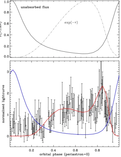
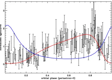
26 Top panel: Theoretical anisotropic inverse Compton emission ("unabsorbed flux", black solid line) and pair production ("exp(−τ)", dashed grey line) above 100 GeV as a function of the orbital phase in LS 5039. Orbital parameters are taken from Casares et al. (2005b). Bottompanel: Gamma-ray light curves expected in the HESS energy band (red solid line, >100 GeV) and in the Fermi energy band (blue solid line,> 1 GeV). HESS data points are shown for comparison and are taken from Aharonian et al. (2006). 62 27 The same as in Fig. 26 (bottom panel) if the compact object is a black hole (i=20◦). 63
28 Theoretical gamma-ray spectra averaged along the full orbit (black solid line), over SUPC (φ≤0.45 and φ >0.9, blue dashed line) and over INFC state (0.45< φ≤0.9, blue solid line). The contribution of synchrotron radiation alone is shown as well in dotted line (black: full orbit, top blue: SUPC and bottom blue: INFC). HESS (filled red bowties) and Fermi (red empty bowtie and black data points) observations are overplotted for comparison. Parameters: i=60◦, p=2, B=0.8 d−1
0.1 G and Lp =1036erg s−1. 64
29 Very-high energy lightcurve observed in LS I+61◦303 (top panel) and PSR B1259−63
(bottom panel). Extracted from Albert et al. (2009) and Aharonian et al. (2009). 65 30 Orbit-averaged spectra (blue line, left panels) and phase-resolved gamma-ray lightcurves
(blue line > 1 GeV, red line > 100 GeV, right panels) in LS I +61◦303 (top panels)
and PSR B1259−63 (bottom panels). Electrons are injected with a power law of index p = 2.5 in both binaries. There is no magnetic field. Fermi (black crosses) and MAGIC observations (red bowtie) are shown for LS I+61◦303, EGRET (grey arrows, upper
limits) and HESS (red bowtie) measurements are also shown for PSR B1259−63. The orbital parameters are taken from Aragona et al. (2009) for LS I +61◦303 and from
Manchester et al. (1995) for PSR B1259−63. 66
31 Simplistic drawing of a pulsar wind. Relativistic pairs of electrons and positrons are generated and accelerated in the pulsar magnetosphere. The wind of pairs is released at the light cylinder radius (RL) and expands radially and freely ("unshocked" pulsar wind)
up to the termination shock ("shocked" pulsar wind) at a distance Rs. At the shock, pairs
32 This diagram depicts the binary system and the geometrical quantities used in the following. An electron from the wind with a Lorentz factor γesituated at a distance r
from the pulsar and R from the companion star, interacts with a stellar photon of energy
ǫ0. 86
33 Total energy losses per electron (blue solid line) as a function of the energy, where ǫ0 = 1 eV and θ0 = 30◦ (bottom), 60◦, 90◦, 90◦ and 150◦ (top). The analytical formula in
the Thomson regime Eq. (38.162) is shown for comparison (red dashed line). 87 34 Lorentz factor of the pairs in the pulsar wind as a function of ψrfor ψ = 30◦ (bottom
lines), 60◦, 90◦, 120◦and 150◦ (top lines), applied to LS 5039 (left panels) and LS I+61◦303
(right panels). Pairs are injected by the pulsar at a Lorentz factor γ0 = 104 (top panels),
105and 106(bottom panels). The massive star is assumed point-like and mono-energetic
and both winds (pulsar and star) are assumed spherical and isotropic. 89 35 These maps show the spatial distribution of the cooled Lorentz factor of the wind in
LS 5039 (left panels) and LS I +61◦303 (right panels) at periastron. Each line gives the
fraction of the energy left in the pairs after Compton cooling: 90% (left lines), 50%, 10% and 1% (right lines) of the injected Lorentz factor γ0. The massive star is shown by a red
semi disk. 90
36 For a finite-size star, the relativistic electron (at the distance r) sees stellar photons
originating within a cone of semi-aperture angle α⋆ =arcsin(R⋆/R)(red dashed line). 91
37 Cooling of the pulsar wind in LS 5039 for γ0 = 104 (left panels) and 106 (right panels).
The solutions for a mono-energetic and point-like star (blue solid lines) are compared with the solutions for a black-body star (red dashed lines, top panels) and a finite-size
star (red dashed lines, bottom panels). 93
38 The observer sees only the radiation from the pairs aligned with the line of sight due to relativistic Doppler beaming effect. Because of the anisotropy of the radiation field set by the massive star, the gamma-ray emission depends strongly on the viewing angle ψ. 94 39 Inverse Compton spectrum emitted by an unterminated and mono-energetic pulsar
wind in LS 5039 at periastron (d≈0.1 AU) with Lp =1036erg s−1at a distance of 2.5 kpc.
Pairs are injected with a Lorentz factor γ0 =104 (top left), 105 (top right), 106(bottom left)
and 107(bottom right). For each energy, the wind is seen with a viewing angle ψ = 30◦
(top line), 60◦, 90◦, 120◦, and 150◦ (bottom line). Pair production is ignored. 95
40 Absorbed inverse Compton spectrum emitted (blue solid lines) by an unterminated and mono-energetic pulsar wind with γ0 = 106 in LS 5039 (left) and LS I+61◦303 (right) at
superior (top, ψ = 30◦) and inferior (bottom, ψ = 150◦) conjunctions. The non-absorbed
spectrum is shown for comparison (dashed red line). Pair cascade emission is ignored. 97 41 The collision between the pulsar wind and the massive star wind produces a bow shock
structure. The shocked stellar wind (red area) and the shocked pulsar wind (green area) are separated by the contact discontinuity (black solid line). The unshocked pulsar wind is limited by the relativistic shock wave front (green solid line) and has an asymptotic
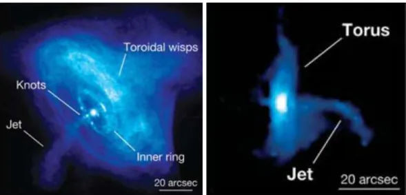
42 X-ray images of the Crab nebula (left, Weisskopf et al. 2000) and the pulsar wind nebula 3C 58 (right, Slane et al. 2004) obtained with Chandra where a jet-torus structure appears clearly. Images Extracted from Gaensler & Slane (2006). 99 43 Angular distribution of the Lorentz factor following Eq. (45.189) normalized to γmwhere
γm/γi ∼ 104. The pulsar pole is oriented along the x-axis where the Lorentz factor
reaches it minimum value γ0and is maximum in the equator plane (y,z) where γ0 ≈γm. 100
44 The pulsar axis (x”) is inclined with respect to the observer at an angle θ. The anisotropic
pulsar wind is represented by the green loops. 101
45 Same as in Fig. 35 for an anisotropic pulsar wind in LS 5039 at periastron. Parameters used: γi =103, γm =106, φ =0 for four different orientations top left (φy=0, φz =π/20),
top right (φy = π/2, φz = 0), bottom left (φy = π/3, φz = π/20) and bottom right
(φy = π/4, φz = π/4). The star is point-like and mono-energetic. The dotted lines
indicate the position of the pulsar, the red dashed line the orientation of the equator and the red disk depicts the massive companion star. 102 46 Same as in Fig. 45 for LS I+61◦303 at periastron. 103
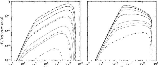
47 Orbit-averaged emission from the free pulsar wind in LS 5039 (top panel) and LS I+61◦303 (bottom panel). The wind is assumed radial, isotropic and mono-energetic
with γ0 = 104 (left), 105, 106 and 107 (right). The gamma-ray emission is calculated
for a terminated (η = 2×10⁻², solid lines) and unterminated wind (dashed lines) for
Lp =1036erg s−1, assuming that the systems are located at 2.5 kpc for LS 5039 and 2 kpc
for LS I+61◦303. Fermi (black data points), HESS and MAGIC (red bowties) observations
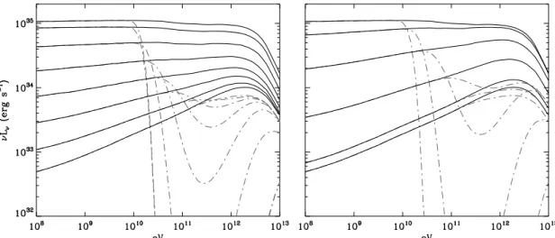
are overplotted. 105
48 Inverse Compton emission in the gamma-ray binaries LS 5039 (left) and LS I+61◦303
from an unshocked pulsar wind. Top: Theoretical orbit-averaged spectrum (blue solid line) for an inclination i = 60◦. Bowties are HESS and MAGIC observations (red,
Aharonian et al. 2006; Albert et al. 2006), black data points show Fermi measurements (Abdo et al. 2009a,b). Middle: Gamma-ray flux integrated over 100 MeV as a function of the orbital phase φ (two full orbits), the Fermi light curve is overplotted for LS I+61◦303.
Bottom: Expected spectral index in the GeV energy band along the orbit. 106 49 The striped current sheet produced by an oblique rotator obtained with the split
monopole model by Bogovalov (1999). Picture extracted from Kirk et al. (2009). 107 50 Kinematics for pair production. The photons annihilate and produce a pair
electron-positron if the total energy available in the center-of-mass frame is greater than the rest
mass energy of the pair. 128
51 Second order Feynman diagram for pair production. 129 52 Variation of the differential cross section dσγγ/d(cos θ1′)for pair production as a function
of cos θ′
1for β =0.3, 0.7, 0.9 and 0.99. 130
53 Geometrical contruction of the center-of-mass frame direction of motion (xcm-axis). 130
54 Geometrical configuration for the computation of the anisotropic pair production kernel.133 55 Spectrum the pair produced in the interaction of a gamma-ray photon of energy
radiation (ǫ0 =1 eV). The collision is head-on here (θ0 = π). The threshold energy for
pair production is≈260 GeV in this configuration. 134 56 Spectrum of pairs created by absorption of primary gamma rays following a power
law energy distribution (photon index−2) and a mono-energetic beam of soft radiation (with ǫ0=1 eV). Spectra are computed for θ0 =10◦, 20◦, 30◦, 45◦, 60◦, 90◦and 180◦. 135
57 Comparison between the analytical (blue line) and the numerically integrated (red dashed line) kernels for an isotropic source of soft radiation. ǫ0 =1 eV and ǫ1 =300 GeV,
500 GeV, 1 TeV and 10 TeV. 136
58 Comparison between the kernel found in Eq. (54.239) and the kernel found by Böttcher & Schlickeiser (1997), Eq. (57.245) where ǫ0=1 eV, and ǫ1 =300 GeV, 500 GeV and 1 TeV
for a head-on collision. 137
59 Cascade of pairs initiated by a primary high-energy gamma ray propagating in a soft
photon field. 142
60 Geometrical quantities used in the model. The primary source injects gamma rays of energy ǫ1 at a viewing angle ψ. These photons are absorbed by the stellar photon of
energy ǫ0 ≈ 2.7kT⋆ at a distance r from the source and yield electron positron pairs
focused along the line of sight due to relativistic beaming effect. 143 61 If the trajectory of the electron deviated by the magnetic field along the Compton
interaction length λic remains within a cone of half opening angle α=1/γe, the cascade
is one-dimensional. 144
62 The primary source injects a density of gamma rays nγ. Between r and r+dr, part of
these photons are absorbed and new are emitted by the pairs produced in the cascade. 145 63 This diagrams depicts qualitatively the depopulation of the energy level Eeto the benefit
of lower energy levels mec2<Ee′ <Ee. 146
64 This diagrams depicts qualitatively the population of the energy level Ee by higher
energy levels E′
e≥ Ee. 146
65 Development of the 1D cascade along the line of sight joining the primary source to the observer. The primary source is point-like, isotropic and injects gamma rays with a
−2 power law energy distribution between 100 MeV and 100 TeV at the location of the compact object in LS 5039. The viewing angle is ψ = 30◦. On the left panels are shown
the full escaping gamma-ray spectra (blue line), the radiation from the cascade only (green line) and the pure absorbed spectrum (red dashed line) for r = R⋆/4 (top), R⋆
(middle) and +∞ (bottom). The corresponding total unabsorbed emission from the
cascade pairs is shown in the right panels. 148
66 The same as Fig. 65 with r → +∞and ψ=30◦, 60◦, 90◦, 120◦, and 150◦. The radiation
from the cascade only is not shown for more readability. 149 67 TeV orbital modulation of 1D pair cascade emission in LS 5039 (red line) as a function
of the orbital phase (two full orbits shown here), and comparison with the primary absorbed flux (blue line). The injection of primary gamma rays is isotropic and constant along the orbit. Both conjunctions are shown with vertical dashed lines (with the orbital
68 Same as in Fig. 67 for LS I+61◦303. The orbital parameters are taken from Casares et al.
2005a). 150
69 Theoretical gamma-ray lightcurves in LS 5039, in the Fermi energy range (flux> 1 GeV leftpanel) and HESS energy range (flux> 100 GeV, right panel). HESS data points are taken from Aharonian et al. (2006). The 1D cascade component (red line) is compared with the primary absorbed contribution (blue line). The sum of both component is
shown by the green line. 151
70 Definition of the geometrical quantities useful for the computation of the density of escaping pairs in binaries. From the compact object point of view (origin), the massive star covers a solid angle Ω⋆. Pairs propagating in the direction of the star (i.e. within Ω⋆)
are not considered in the calculation of the escaping density of pairs. 152 71 Left panel: Mean energy of escaping pairs at infinity as a function of the viewing angle ψ.
Rightpanel: Density of escaping pairs in the cone of semi-aperture angle ψ as a function
of ψ. 152
72 Emission from a mono-energetic free pulsar wind in LS 5039 at superior conjunction (ψ = 30◦) for γ0 = 104(left) and 106 (right) with L
p = 1036erg s−1. The exact solution
(i.e. keeping track of stochastic losses for the electrons, green line) is compared with the approximate solution (continuous losses approximation, red dashed line). The solution with 1D pair cascading is shown by the blue line. 153 73 Three-dimensional "isotropic" pair cascade (grey domain) is initiated if the magnetic field
is strong enough to confine locally pairs B >Bminor the cascade would be "anisotropic",
but it should not exceed B < Bmaxor pairs will emit mainly synchrotron radiation and
the cascade would be "quenched". Pairs remain in the system if the magnetic field is above the dashed line. Left: LS 5039, right: LS I+61◦303, at periastron for both systems. 171
74 Primary gamma rays injected at r≡ 0 in the direction (θ, φ) produce pairs at r from the
source and R from the massive star center. 172
75 Density of pairs produced by the annihilation of the primary gamma rays (injected at r ≡ 0 with a−2 power law energy distribution) with stellar photons at r = R⋆/4 (top
left), R⋆/2, R⋆and 2R⋆ (bottom right) in LS 5039. In each panel, the spectrum of pairs is
computed for θ =30◦ (top, dashed line), 60◦, 90◦, 120◦ and 150◦(bottom, dotted line). 173
76 This map gives the mean Lorentz factor of the pairs at their creation in LS 5039 at superior conjunction. The primary source is a−2 power law with a high energy cut-off at 100 TeV. The star (red disk) is assumed mono-energetic and point-like but the eclipse is taken into account (black region behind the star with respect to the source). 174 77 Top panels: This map shows the fraction of the gamma-ray flux left after pair production
e−τγγ(r,θ). Bright region are transparent and black regions are opaque. Bottom panels:
Density of secondary pairs given by Eq. (66.278). The white lines gives the fraction of the absorbed primary gamma-ray flux. In both maps, the primary source injects photons of energy ǫ1 = 100 GeV at the compact object location (r ≡ 0) in LS 5039 (left panels)
and LS I+61◦303 (right panels), at periastron for both systems. The eclipsed region
by the massive star (red semi disk) is delimited by a white dashed line. Distances are
78 Same as Fig. 77 with ǫ1 =1 TeV. 176
79 Same as Fig. 77 with ǫ1 =10 TeV. 176
80 The binary system is seen by a distant observer with a viewing angle ψ. Secondary pairs are secondary sources of gamma rays seen at an angle ψobs. 177
81 The massive star excludes part of the volume to the primary gamma-ray source (grey
area) and to the observer (red area). 177
82 Left panel: Escaping radiation spectrum (blue line) for ψ= 30◦, 60◦, 90◦, 120◦ and 150◦.
The primary source is point-like, isotropic and injects gamma rays with a−2 power law energy distribution between 100 MeV and 100 TeV at the location of the compact object in LS 5039 (dotted line). The radiation from the pure absorbed spectrum (red dashed line) is shown for comparsion. The emission from secondary pairs only is shown in the
rightpanel. 179
83 TeV orbital modulation of 3D pair cascade emission in LS 5039 (red line) as a function of the orbital phase (two full orbits shown here), and comparison with the primary absorbed flux (blue line) and the full 1D cascade flux (red dashed line). The injection of primary gamma rays is isotropic and constant along the orbit. Both conjunctions are shown with vertical dashed lines (with the orbital parameters found by Casares et al.
2005b). 180
84 Spatial distribution and intensity of the very high-energy (> 100 GeV) radiation produced by the first generation of pairs in the 3D cascade in LS 5039 as observed by a distant observer (whose direction is indicated by a white solid line, top panels). Distances are normalized to the orbital separation d. The system is viewed at superior (left) and inferior conjunctions (right). Each map is a slice of the 3D cloud of gamma rays in the three orthogonal planes: front view (plane containing the observer and both stars, top panels), top view (middle) and right view (bottom). The primary source lies at the origin. The eclipsed regions by the massive star (red disk) are delimited by white dashed lines. The injection of the primary gamma rays is the same as in Fig. 82. 181 85 Left panel: The same as in Fig. 82 (right panel) for the second generation of pairs in
the cascade only. Right panel: ratio of the second generation to the first generation
gamma-ray flux in the cascade as a function of energy. 182 86 Left panel: Full cascade emission computed with the Monte Carlo code (blue solid line)
in LS 5039 for ψ = 30◦ and 150◦. Comparison between the semi-analytical (red dashed
line) and the Monte Carlo (red solid line) results for the first generation of gamma rays only. The primary source is shown with a dotted line. Right panel: This plot shows the relative contribution from the primary absorbed flux (red dashed line), the first generation (red solid line) and from extra-generations (i.e. > 1, green line) to the total escaping gamma-ray flux (blue line) in LS 5039 for ψ = 30◦. The right panel uses only
results from the Monte Carlo code. Synchrotron radiation is ignored. 183 87 The same as in Fig. 83 where the 3D cascade radiation is computed with the Monte Carlo
approach for all the generations (red solid line). The radiation from the first generation (Monte Carlo result) is plotted as well for comparison (red dotted line). 183
88 Left panel: Effect of the ambient magnetic field on the cascade radiation (first generation). The cascade is computed with the same parameters (semi-analytical approach) as used in Fig. 82 for ψ=30◦with an uniform magnetic field B=0 (top) , 1, 3, and 10 G (bottom).
The cascade radiation (dashed red line) is compared with the injected (dotted line) and the full escaping gamma-ray spectra (blue solid line). Right panel: Effect of the magnetic field on the contribution from extra-generations in the cascade for B = 0, 3, and 10 G
and ψ = 90◦. The full escaping gamma-ray spectrum (Monte Carlo approach) with all
generation (solid blue line) is compared with the one-generation cascade approximation
(red dashed line). 184
89 Theoretical TeV lightcurve in LS 5039 (two full orbits, blue solid line) for i = 60◦ (top
panel) and i = 40◦ (bottom panel), where 3D pair cascade radiation is computed with
the Monte Carlo code for a finite-size and black-body companion star. The contribution from the cascade only (red solid line) and HESS data points are shown for comparison. Lightcurves are averaged in phase interval of width ∆φ = 0.1. The orbital parameters are taken from Casares et al. (2005b). Conjunctions are indicated by dotted lines. 186 90 Theoretical gamma-ray spectra in LS 5039 with i = 40◦. Spectra are averaged over the
"SUPC" (0.45 < φ < 0.9, green dashed line) and "INFC" (φ < 0.45 or φ > 0.9, green solid line) states as defined in Aharonian et al. (2006), and over the whole orbit (blue line). Fermi (data points and red contours) and HESS (red bowties) measurements are overplotted. The full 3D pair cascade emission is included (Monte Carlo calculations). The ambient magnetic field is chosen small B<1 G. 187 91 Spatial distribution of the gamma-ray flux in LS 5039 at periastron (top panels), superior
conjunction, apastron and inferior conjunction (bottom panels). These maps show the cascade gamma-ray emission in the high-energy (flux> 1 GeV, middle panels) and very-high energy bands (flux> 100 GeV, right panels) from the first generation only. These calculations were performed with the semi-analytical method. Each maps are centered to the massive star center. The orbit seen with an inclination i = 60◦ is shown
on the left panel. The position of the compact object in the orbit is indicated by red solid
line and a black dot. 188
92 The gamma-ray source may not coincide with the compact object location (green circle) but could be localized further away at a distance d′ from the massive star center in the
orbital plane (blue circle in the "pulsar wind"), or above the orbital plane at an altitude h
(blue circle in the "jet"). 189
93 Same as in Fig. 89 for i = 60◦, where the TeV primary source is located in the orbital
plane with d′ = 3d (top panel) or above and perpendicular to the orbital plane at an
altitude h = R⋆(bottom panel). 190
94 Theoretical spectrum of the cascade radiation (first generation) averaged over the orbit with a uniform ambient magnetic field B =0.1, 1, 5 and 10 G. Suzaku (Takahashi et al. 2009), Fermi (Abdo et al. 2009b) and HESS (Aharonian et al. 2006) observations are shown
for comparison. 191
95 Emission processes seen in the observer frame (left panel) and in the comoving frame of the flow (right panel). Waves represent photons and the green thick arrow shows the
direction of motion of the flow with a bulk Lorentz factor Γ > 1. The boost from the observer to the comoving frame is along the z-axis. 208 96 Effect of the Doppler boost on synchrotron radiation flux for a power law spectrum. The
flux is increased by a factorD3
obsand the power law is shifted in energy by a factorDobs. 210
97 Doppler factorDobsas a function of the cosine of the angle between the observer and the
flow µobsfor β = 0 (red dahed line), 0.1, 0.5 and 0.9 (top). The flux is forward boosted
by the flow (Dobs > 1) in a cone of semi aperture angle∼ 1/Γ, otherwise the flux is
deboosted (Dobs <1). 210
98 Doppler factorDobs as a function of β for ψobs = 0◦ (dashed blue line) 20◦, 30◦, 60◦, 90◦
and 180◦. The flux is deboosted (D
obs <1) if Γ&1/ψobs. 211
99 Boosted anisotropic inverse Compton emission in the observer frame (blue solid lines) for ψobs = 180◦ and θf low = 0◦ for a bulk velocity of the flow (from top to bottom)
β = 0, 0.1, 0.3, 0.5 and 0.9. Pairs are injected with an isotropic power law energy distribution with γ−=102and γ
+=107, and with an index p=2. The red dashed lines
give the analytical solution found in Eq. (80.316) valid in the Thomson limit. The source of soft photon is point like with a black body spectrum of temperature T⋆ =39 000 K in
the observer frame. 213
100 Inverse Compton flux as a function of ψobs for θf low = 0◦and for a bulk velocity of the
flow β =0 (top left panel), 0.1 (top right panel), 0.3 (bottom left panel) and 0.5 (bottom right panel). The orbital phase is defined here as ψobs/2π so that ψobs = 180◦ correponds to
0.5. Curves are normalized and integrated over energies above 100 MeV (blue lines) and
above 100 GeV (red lines), with T⋆ =39 000 K. 214
101 Geometry in gamma-ray binaries for the calculation of the Doppler-boosted emission. The shocked pulsar wind is collimated, inclined at an angle θf low with respect to the
massive star-pulsar direction and is contained in the orbital plane. A distant observer sees the system with a viewing angle ψobs. The emission originates from a very small
region (blue disk) at the pulsar location. 219
102 Orientation of the shocked pulsar wind in LS 5039. In this system, the flow is assumed
radial. 220
103 Left panels: Theoretical non-thermal radiation expected in the one-zone leptonic model Dubus et al. (2008) with no Doppler boost β=0. SUPC and INFC spectra are compared with Suzaku (Takahashi et al. 2009), Fermi (Abdo et al. 2009b) and HESS (Aharonian et al. 2006) bowties on the top panel. The expected very-high energy (middle panel) and X-ray (bottom panel) lightcurves are also shown. Right panels: The same as in the left panels with a Doppler boost β=1/3 and θf low=0◦. 221
104 Orientation of the shocked pulsar wind in LS I +61◦303. In this system, the flow is
assumed tangent to the orbit in the opposite direction of the orbital motion. 222 105 Left panels: Theoretical synchrotron (red lines) and inverse Compton radiation (blue lines)
expected in a one-zone leptonic model as a function of the orbital phase in LS I+61◦303
(two full orbits). Electrons are injected with a constant power law energy distribution of index p= 2 and are bathed in a constant magnetic field along the orbit. In the top panel, synchrotron and the inverse Compton fluxes are calculated with β = 0. In the last two
panels, β=1/3 and the flow is assumed tangent to the orbit. Inverse Compton emission is computed with the analytical formula found in Eq. (80.316) (Thomson limit). The exact inverse Compton flux (with Klein-Nishina effects) computed above 100 GeV is shown in the bottom panel. The absorbed Compton gamma-ray lightcurve is shown with dashed line. The orbital parameters are taken from Aragona et al. (2009) and the origin φ = 0 was chosen at periastron for this plot, i.e. 0.275 should be added to the phasing used in Aragona et al. (2009) and in the text. Right panels: Application to PSR B1259−63 with
β=0 (top), 1/3 (middle) and 0.9 (bottom). 223
106 Left panel: Geometry of the jet in Cygnus X−3. The compact objet produce a two-sided inclined jet with a relativistic velocity βββ = ±βej. Stellar photons are upscattered to high
energies by energetic electrons localized at two symmetric positions at an altitude H in the jet (blue disk) and counter-jet (red dashed disk). Right panel: Top view of the
compact object orbit. 239
107 High-energy gamma-ray flux (> 100 MeV) in Cygnus X−3 as a function of the orbital phase (two full orbits here) for the black hole solution. The solution shown (blue solid line) has a χ2 = 2.9 for a set of parameters β = 0.45, H = 8.5×1011 cm,
φj = 12◦, θj = 106◦ and with a total power in electrons Pe= 1.12×1038 erg s−1(where
γ−=103). The contributions from the jet (red solid line) and the counter-jet (red dashed
line) are shown as well for comparison. The folded Fermi lightcurve data points are
taken from Fermi LAT Collaboration (2009). 241
108 Distribution of good fit models in the 90% of condidence region of the χ2 statistics for
the black hole solution (left panels) and for the neutron star solution (right panels) for the parameters β (top panels), H, φj and θj (bottom panels). The filled regions gives the
number of model such as the total power injected into pairs Pe is. Ledd (light grey
region),. 10−1L
edd (grey region) and. 10−2Ledd (dark grey region). The Eddington
luminosity is Ledd=2×1039erg s−1for the black hole and Ledd=2×1038erg s−1for the
neutron star. 242
109 Effect of the precession of the jet on the high-energy emission and modulation in Cygnus X−3. From the best fit solution (black solid line) with θj = 319◦, only the
azimuth angle is changed to (from dark to light grey line) θj =31◦, 103◦, 175◦ and 247◦. 243
110 Geometry of a standard accretion disk. The compact object is located at the origin and the gamma-ray source above the accretion disk. Gamma-ray photons propagating towards the observer can be absorbed by thermal photons from the disk. 244 111 Gamma-ray opacity map exp(−τγγ)as a function of the viewing angle ψ and the altitude
of the gamma-ray source z in the jet, for r = 0 (along the axis of the accretion disk). Bright regions indicate low opacity τγγ ≪1 and dark regions high opacity (τγγ ≫ 1).
The gamma-ray photons have an energy ǫ1 =1 GeV and propagate above an accretion
of inner radius Rin=107cm and external radius Rext=1011cm with ˙M =10−8M⊙yr−1.
The white dotted line indicates z =Rinand the black dotted line z=d. 245
112 Same as in Fig. 111 in the(r, z)plane for a viewing angle ψ=0◦ (left panel) and ψ=45◦
113 Gamma-ray opacity as a function of the gamma-ray energy ǫ1 for z = 100Rin on axis
1 Physical and orbital parameters in gamma-ray emitting binaries adopted in this thesis. 5 2 Parameters used for the modeling of the Compton emission shown in Fig. 48. 107
Part
I
Introduction
1 What is this thesis about? 3
1
What is this thesis about?
Outline
1. The cosmic accelerators uncovered by the gamma-ray astronomy . . . 3 2. Binary systems in the gamma-ray sky! . . . 4 § 1. Gamma-ray binaries . . . 4 § 2. Microquasars. . . .6 3. Objectives of this thesis: What we want to understand . . . 7 4. Guidelines: How is this thesis constructed? . . . 8
1. The cosmic accelerators uncovered by the gamma-ray
astronomy
T
HERE IS EVIDENCE that particles are accelerated up to ultra-high energies (> 1019eV)in our Universe. How and where these energetic particles are accelerated are still highly debated questions. Thanks to space and ground-based facilities, gamma-ray astronomy has firmly identified during the last couple of years many astrophysical objects where particles are accelerated to high (>100 MeV) and very-high (>100 GeV) energies. Gamma rays are very energetic photons (&100 keV) produced when these high-energy particles interact or decay. Gamma-ray astronomy reveals the most energetic phenomena taking place in our Universe related to extreme physical conditions, as for instance high-energy densities, relativistic outflows or strong gravitational fields. The gamma-ray sky is also highy variable. This behavior is associated with the activity and the physics of compact objects such as neutron stars or black holes.
Gamma-ray astronomy is undoubtedly living its golden age today where space and ground based telescopes cover the sky simultaneously over 6 orders of magnitude in energy range (from 100 MeV to 100 TeV) with unprecedented sensitivity and angular resolution. We are facing a period in the history of high-energy astrophysics when the gamma-ray astronomy is mature enough to make reliable and direct observations of the cosmic accelerators. More than a hundred sources1have been detected by the third generation of Atmospheric Cherenkov telescopes such as HESS, MAGIC and VERITAS above 1 TeV and more than a thousand sources
have been detected at GeV energies by the space gamma-ray telescopes Fermi and AGILE (see e.g. the first Fermi LAT source catalog, The Fermi-LAT Collaboration 2010). The extragalactic gamma-ray sky is dominated by Active Galactic Nuclei (or AGN). The detection of gamma-ray bursts (or GRBs) and a few starburst Galaxies have also been reported. In our Galaxy, most of gamma-ray sources are pulsars, pulsar wind nebulae and supernova remnants but many other sources remain unidentified. Amongst the Galactic gamma-ray sources, there are a few of binary systems. This thesis is focused on these systems.
2. Binary systems in the gamma-ray sky!
Four gamma-ray sources have been firmly associated with Galactic binary systems, namely: LS I+61◦303, LS 5039, PSR B1259−63 and Cygnus X−3. These identifications are definitively
established thanks to the good localisations of the sources in the sky and to the very-high detection significance level (high signal/noise ratio). These gamma-ray sources are time-variable and demonstrably modulated on the orbital period in some cases (Aharonian et al. 2006; Albert et al. 2009; Aharonian et al. 2009; Abdo et al. 2009a,b; Fermi LAT Collaboration 2009). This is the main observational signature of these systems. These gamma-ray emitting binaries are composed of a massive non-degenerated star (Be, O or Wolf-Rayet) and a compact object. The parameters of these binaries (orbit, distance, companion star, ...) are known from optical spectroscopy and are summarized in Tab. 1 (see also the orbits in Fig. 1).
The TeV gamma-ray source HESS J0632 + 057, serendipitously discovered by HESS (Aharonian et al. 2007), might be also associated with a binary system (Hinton et al. 2009), but no orbital modulation has been reported yet even though the source exhibits some variability (Acciari et al. 2009). A TeV gamma-ray flare from Cygnus X−1 has been reported by the MAGIC collaboration (Albert et al. 2007) but with a low significance. In addition, the detection of GeV gamma-ray flares have been claimed by the AGILE collaboration (Sabatini et al. 2010), but these observations have not been confirmed by Fermi. I will not consider these two binary systems as firmly established gamma-ray emitting binaries in this thesis.
In this sample of binaries, we have two distinct classes of objects:
• Gamma-ray binaries: LS 5039, LS I +61◦303 and PSR B1259−63 (and HESS J0632+
057 ?).
• Microquasars: Cygnus X−3 (and Cygnus X−1 ?).
I give below the main properties of these objects and intend to depict the scenario of emission considered in this thesis for "gamma-ray binaries" and for "microquasars".
§ 1. Gamma-ray binaries
These systems emit non-thermal radiation from radio up to 10 TeV. Their non-stellar luminosity is maximum above 1 MeV, hence the name given to these systems "Gamma-ray binaries" (Dubus 2006b). The gamma-ray emission observed is steady with a low orbit-to-orbit variability. The TeV luminosity measured in these systems is high Lγ ∼ 1032-1033 erg s−1and is of the order of the
X-ray luminosity. In PSR B1259−63, the compact object is a young 48 ms pulsar. Radio pulses are detectable but vanish near the passage to periastron, probably due to free-free absorption in
TAB. 1. Physical and orbital parameters in gamma-ray emitting binaries adopted in this thesis.
System PSR B1259−63 LS I+61◦303 LS 5039 Cygnus X−3
GeV or TeV emission? TeV GeV and TeV GeV and TeV GeV
Companion star type Be Be O WR
Stellar Temperature T⋆ (in K) 27 000 22 500 39 000 100 000
Stellar radius R⋆ (in R⊙) 10 10 9.3 0.6−2.3 (?)
Star mass M⋆(in M⊙) 10 12 23 5−50 (?)
Distances (in kpc) 1.5 2 2.5 7
Compact object1 NS NS or BH NS or BH NS or BH
Orbital period Porb(days) 1237 26.5 3.9 0.2
Eccentricity e 0.87 0.537 0.337 0
Inclination i (degree) 35 ? ? ?
Periastron angle ω (degree) 139 40.5 236 0
FIG. 1. Top view of the compact object orbit (blue line) in Cygnus X−3(top left), LS 5039 (top right), LS I+61◦303
(bottom left) and PSR B1259−63(bottom right). The red filled disk represents the massive star at scale in the system and the back solid line indicates periastron. The observer sees the orbit from the bottom.
the Be stellar wind (Johnston et al. 1992). In LS 5039 and LS I+61◦303, the nature of the compact
object is still unknown.
Maraschi & Treves (1981) suggested that the non-thermal emission in LS I +61◦303 arises
from the interaction of the relativistic wind generated by a young fast-rotating pulsar with the companion star wind (note that this scenario has been first proposed for Cygnus X−3 by Bignami et al.1977). A small-scale pulsar-wind nebula is formed in the system. In PSR B1259−63, this scenario is most probably at work regarding the nature of the compact object in this system (Tavani et al. 1994; Kirk et al. 1999), but this is not clear for the other two binaries. However, the three systems share the same spectral and temporal features as depicted above. This argues in favor of a common scenario (Dubus 2006b). Gamma-ray binaries may all harbor a young fast-rotating pulsar. This is the "pulsar wind nebula" scenario. In addition, LS 5039 and LS I+61◦303
do not show any sign of accretion (see the discussion in Dubus 2006b), arguing against accretion-power scenario. However, some models have been proposed in the "microquasar" scenario (see next section) i.e. where the high-energy emission orginates from a relativistic jet powered by accretion on a black hole (see e.g. the works by Dermer & Böttcher 2006; Paredes et al. 2006; Romero et al. 2007).
In the pulsar wind nebula scenario (see the sketch in Fig. 2), high-energy electron-positron pairs are injected by the pulsar in a cold relativistic wind ("unshocked", green area in Fig. 2). The wind propagates freely up to the termination shock created by the collision with the stellar wind. In the "shocked" pulsar wind (red area in Fig. 2), pairs are randomized, accelerated and radiate non-thermal radiation. If the massive star wind is strong, the pulsar wind may be confined in a collimated outflow. A comet-like tail spiraling around the system forms in the system due to the orbital motion of the pulsar. This scenario provides a common framework to interpret the spectral and temporal behaviors in these systems.
The study of gamma-ray binaries has important implications. The wind of isolated pulsars is confined by the material of its supernova remnant on parsec scales. In gamma-ray binaries, the pulsar wind is confined to sub-AU scales by the massive star wind. These systems provide a novel environment for the study of pulsar winds at very small scales. The formation, the composition and the acceleration processes in pulsar winds are still poorly understood today. These important issues will undoubtedly benefit from the study of gamma-ray binaries.
§ 2. Microquasars
Microquasars are accreting binary systems with relativistic jets which are similar to those found in AGN or GRBs but on Galactic scales. In spite of the huge different spatial scales, AGN and microquasars exhibit many similarities in their temporal and spectral behaviors, suggesting that the same underlying physics is at work. In such systems, the primary source of energy is gravitational. Material from the normal star is accreted on the compact object (neutron star or black hole). Part of the accretion power is channeled in the formation and acceleration of a relativistic jet (see the diagram in Fig. 3). The observation of non-thermal radiation in radio up to X-rays from microquasar jets provides good evidence for particle acceleration up to 10 TeV (Corbel et al. 2002). The firm detection of Cygnus X−3 in gamma rays by Fermi gives the definitive evidence that microquasars emit high-energy gamma rays. Contrary to gamma-ray binaries, the gamma-ray luminosity is lower than the X-ray luminosity (Lγ .10−2LXin Cygnus
X−3). In addition, the gamma-ray emission is transient and related to major ejections events in the relativistic jet. The study of microquasars in gamma rays is particularly interesting as these
+ e /e− + e /e− star stellar wind γ Pulsar UNSHOCKED SHOCKED γ Massive Observer Pulsar γ
ψ
ZOOM SHOCKED UNSHOCKEDFIG. 2. This sketch depicts the main components in gamma-ray binaries involved in the non-thermal emission
mechanism, in the pulsar wind nebula scenario (see the text for explanations).
systems provide a nearby and well constrained laboratory to understand the accretion-ejection mechanisms and the acceleration processes in relativistic jets. This also benefits to the study of AGN.
3. Objectives of this thesis: What we want to understand
This thesis is dedicated to the modeling of the high-energy radiation emitted by gamma-ray binaries and microquasars. The study presented here was triggered by the intriguing HESS observations of the gamma-ray modulation in LS 5039. My thesis focuses on the theoretical modeling of the gamma-ray variability (flux and spectrum) in gamma-ray emitting binaries. For this, it is important to take into account the full complexity of the geometry in all the relevant high-energy processes. The ultimate goal of this thesis would be to answer the following questions:
1. What are the relevant processes in compact binaries at high energies? 2. Where does the gamma-ray orbital modulation come from?
3. What is the nature of the compact object in these systems? 4. Where does particle acceleration take place?
observer
star
companion
γ
γ
γ
γ
γ
γ
γ
γ
γ
accretion disk
shock
ISM
counter−jet
jet
e /e− +stellar wind
pFIG. 3. Sketch of a microquasar and of its different components. Energetic particles are accelerated in the relativistic
jet and radiate high-energy emission.
6. What is the physics at work in pulsar winds? 7. What is the emission from relativistic outflows?
4. Guidelines: How is this thesis constructed?
The manuscript is divided into 5 distincts parts and 12 chapters. Below, I give an overview of each part and indicate the related questions (out of the ones listed in the previous section) for which it aims to answer.
Part I presents the main objectives of this thesis (this Chapter) and introduces the main processes considered in high-energy astrophysics (Chapter 2). The main objective of this part is to distinguish amongst the known high-energy processes which one are the most relevant in binaries (Question 1). Hadronic and leptonic origin of the high-energy gamma rays are discussed. Chapter 2 provides the main equations for the computation of high-energy processes which will be useful throughout this thesis. This toolbox is however incomplete and is not always appropriate in our context. In consequence, I had to develop specific theoretical tools adapted for the modeling of the high-energy emission in a binary environment. These tools are presented in Chapter 3, 6 and 9 at the beginning of each part (II, III and IV).
Part II is dedicated to the modeling of the gamma-ray emission from gamma-ray binaries, in the framework of the pulsar wind nebula scenario. Chapter 4 will focus on the emission from the "shocked" pulsar wind and Chapter 5 on the emission from the "unshocked" wind. The goal of this part is to see whether the pulsar wind nebula model provides a viable scenario to account
for gamma-ray observations and in particular the modulation (Question 2). The objective is also to formulate new constraints on the physics of pulsar winds such as the magnetic field or the particle energy distribution (Question 5, 6 & 7).
In LS 5039, gamma-ray absorption is very high and leads to the creation of many electron-positron pairs. These particles can initiate a cascade of new pairs and contribute significantly to the total gamma-ray flux. The model of the shocked pulsar wind (Chapter 4) fails to account for the observed TeV gamma-ray flux where gamma-ray absorption is very high. The high-energy radiation reprocessed by the cascade could reduce significantly the gamma-ray opacity in LS 5039, and could explain the observed TeV gamma-ray flux.
Part III focuses on the modeling of pair cascade emission in gamma-ray binaries, particularly in LS 5039. As a first attempt and in order to quantity the relevance of this process, I present a one-dimensional model for the cascade radiation in binaries (Chapter 7). I will show that this type of cascade is not realistic but provides an upper limit of the cascade emission where absorption is very high. In LS 5039, a more realistic assessment of the gamma-ray emission from the cascade is required. I developped a three-dimensional model for the cascade in gamma-ray binaries in collaboration with Julien Malzac which I apply to the case of LS 5039 (Chapter 8). The main objective is to explain the amplitude of the TeV gamma-ray modulation (Question 2). I investigate also in this part the effect the ambient magnetic field and the effect of the location of the gamma-ray emitter in LS 5039 (Question 4).
Part IV describes the effects of a relativistic bulk motion on radiative processes (Question 7) in the context of pulsar winds in gamma-ray binaries (Chapter 10). In the classical model of pulsar winds, the shocked pulsar wind has a mildly relativistic bulk velocity. Relativistic Doppler-boosting effects should change the high-energy emission and change the modulation (Question 2). These effects are precisely investigated in this part. I formulate constraints on the bulk velocity of the flow (Question 6).
In Part IV, I present also a new model for the gamma-ray emission in the microquasar Cygnus X−3 (Chapter 11). The main objective is to explain the origin of the GeV gamma-ray orbital modulation in this system (Question 2). The fit of the theoretical to the observed lightcurve constrains the geometry and the physics of the jet in Cygnus X−3 (Question 3, 4, 5 & 7).
Part V briefly summarizes the main results obtained in this thesis. The list of questions given in the first chapter is updated and addressed to future investigations.