Deterministic Approximations to Co-Production+ Problems with Service Constraints
Gabriel R. Bitran* Thin-Yin Leong**
MIT Sloan School Working Paper #3071-89-MS
August 1989
*Sloan School of Management,
Massachusetts Institute of Technology, Cambridge, MA 02139.
**Sloan School of Management, and National University of Singapore,
Republic of Singapore.
+This research was partially supported by "The Leaders for Manufacturing Program".
I
Deterministic Approximations to Co-Production Problems with Service Constraints.
Gabriel R. Bitran* and Thin-Yin Leong**
Abstract
We study production planning problems where multiple item categories are produced simultaneously. The items have random yields and are used to satisfy the demands of many products. These products have specification requirements that overlap. An item originally targeted to satisfy the demand of one product may be used to satisfy the demand of other products when it conforms to their specifications. Customers' demand must be satisfied from inventory a% of the time. We formulate
the problem with service constraints and provide near-optimal solution to the problem with fixed planning horizon. We also propose simple heuristics for the problem solved with a
rolling horizon. Some of the heuristics performed very well over a wide range of parameters.
*Sloan School of Management, Massachusetts Institute of Technology, Cambridge, MA 02139.
**Sloan School of Management, and National University of Singapore, Republic of Singapore.
Deterministic Approximations to Co-Production Problems with Service Constraints.
Gabriel R. Bitran and Thin-Yin Leong
1. Introduction
This paper examines multi-period multi-item production planning problems in environments with stochastic process yields and substitutable demands. The outputs of the process have characteristics that vary in a broad band covering the needs of several customers. The functional form of the products desired by different customers are the same but their
performance requirements are different. These requirements may overlap such that units produced for one customer may be used selectively to fill
another customer's demand. Customers' demands must be satisfied from inventory % of the time.
Such situations are often encountered in practice. Especially notable are those in the high-volume components manufacturing and petro-chemical processing industries. The semi-conductor and electronic components
sectors, in particular, are characterized by high yield variabilities, and produce products that have different specifications and applications. For example, a component part that goes into high technology applications like aerospace instruments has tighter specification requirements than a similar part that is used in consumer products.
The units produced by the manufacturing process can be classified into a set of finite number of item categories according to the ranges of their specified characteristics. The total yield rate of the manufacturing process is probabilistic. Hence the percentage of acceptable units and the relative proportions of items in each production lot can be different from run to run. The variations of the proportions among the items are
correlated. The units are classified into items to simplify inventory management. The demand for products from customers is met by selecting the
items that conform to the needed requirements. The requirements met by one item may also be satisfied by items that are defined by more stringent specifications. In this way, product demands are substitutable.
This paper is based on a study performed at a custom semi-conductor manufacturing facility. Current practice at this facility does not
distinguish items from products. Production runs are made to order because of the large number of product configurations. The paper is organized as follows. The literature is briefly reviewed in section 2, followed by the detail problem description and model assumptions. The model formulation and analytical results are presented in section 4. Heuristics motivated by the
analyses are described in section 5. The next section reports computational results and comments on implications of the results. The paper ends with a
summnary and conclusions.
2. Literature Review
The general class of problems studied in this paper was proposed by Bitran and Dasu [1989]. They identified a class of problems with multiple items, stochastic yields, and, more importantly, interchangeability of items to satisfy customers' demand. They framed a multi-period model with dynamic deterministic demand; production, shortage and holding costs; and product substitution structure. Drawing from the insights of the two period problem, a class of heuristics was provided for solving the multi-period problem with no capacity constraint.
Until recently, stochastic yield problems have received little attention in the literature. Whenever uncertainty is incorporated in the models, it is usually related to demand variability. Even these have
certain peculiarities. Production planning problems with uncertainties usually assume that production capacity is unconstrained. This point was highlighted in Bitran and Yanasse [1984]. Problems of this type have been thoroughly investigated in the field of inventory control. The
production/inventory management literature splits into the two main
streams: 1)capacitated problems with deterministic demands or 2)stochastic demands and/or yields problems with no capacity constraint.
Papers that studied yields related problems include Shih [1980]; Karmarkar, and Lin [1986]; Mazzola, McCoy, and Wagner [1987]; Moinzadeh,
and Lee 1987]; Lee and Yano [1988]; Gerchak, Vickson, and Parlar [1988]; and Henig, and Gerchak 1989]. All these problems focussed on the single item case. Yano, and Lee 1989] review the lot-sizing problem when the yields are random. They reported finding little research done on multi-period problems. The measure of performance in most of the papers, the authors encountered, seek to minimize expected costs and very few have constraints on measures of service. The latter, it seems, is because their inclusion make the problem intractable rather than being irrelevant in the problem context.
Multi-item models usually consider decisions related to the
production of items one at a time or in coordination. The decision-makers, in these problems, decide how much of each item to produce. Deuermeyer, and Pierskalla [1978] studied processes with co-production; that is, multiple products produced simultaneously or product with by-products. They made no
distinction between items and products since it did not matter in their instance. Deuermeyer, and Pierskalla [1978] consider two items and two processes. One of the two processes makes two items simultaneously, with fixed item proportions while the other can produce one given item. The
model can be generalized to m processes and n items. The products' demand is stochastic with no substitution allowed and there is no capacity
constraint.
Almost all of the stochastic production planning/inventory control models have penalties for product shortages. Managerially, it is sometimes difficult to quantify what the shortage costs comprise as well as their magnitudes relative to other costs. In most instances, the production
facilities are evaluated on their ability to meet demand. Hence, it is more appropriate, in these instances, to model directly the service
requirements. Chance constraints are often used for this purpose. Bitran and Yanasse [1984] provided deterministic approximations to the production problem with stochastic demands. Service constraints were used in place of shortage costs. The service constraints were formulated as chance
constraints and were converted into their deterministic equivalent. The problem was approximated by a deterministic linear program. The authors provided parametric relative bounds for their approximations. The relative errors are small for probability distributions commonly encountered in practice.
Our model generalizes Bitran and Dasu [19891's model to T periods and multiple items with a general product demand substitution structure. In place of shortage costs, we introduced service constraints. The approach we take follows from the work of Bitran and Yanasse 1984]. In contrast, we have uncertainty in the yield rates with given demands whereas they assumed
fixed yield rates with stochastic demands. Our problem assumes the production of multiple items but this differ from their multi-item
extension in that we have co-production of the items and our products' demand is substitutable. As in Bitran and Yanasse [1984], we use Jensen's
inequality to provide relative error bounds. For a more complete
bibliography of previous studies and related problems, see Bitran and Dasu [1989], Bitran and Yanasee [1984], and Yano and Lee 1989].
3. Problem Description and Model Assumptions
In studying the co-production problem with stochastic yield we encountered the following types of management decisions: process-product structuring decisions and production planning decisions. A production
process may be set for a specific product. However, because of variation in the output characteristics, by-products, for which there may be demand, will be produced. Hence, instead of having processes specified for each individual product, a sub-set of processes can be identified with each process targeted towards a group of products. Each process produces a subset of items. The items are used to satisfy products' demand. The chain relationship is shown below. The first set of decisions consists of
determining what processes to select and what products are covered by each. These higher level decisions will be addressed in a forthcoming paper.
Figure 1. Process-Item-Product Chain Relationship.
For a given sub-set of products, and their pre-selected process, the production planning decisions are: l)how much to produce and 2)how to allocate the inventory of items to the products. We consider, in this paper, the production planning problem under the following assumptions:
a. A multi-period model with finite planning horizon. Decisions are made
I
at the beginning of each period. Production is instantaneous or has a leadtime of a finite number of periods. The demands are deterministic and dynamic. Without loss of generality, there are no initial inventories of items. Shortages are backordered. Service requirements for meeting each product's demand are given. These are expressed as meeting or exceeding given probabilities of satisfying demand.
b. Holding and production costs are incurred in each period. All cost functions are proportional to the number of units and have the same
constants of proportionality for each period. Shortages are not explicitly penalized. Undesired units may be sold for a small salvage value and
revenue from this source is assumed to be negligible. Because of the above, to maximize profit we need only mnimize the total cost.
c. The joint yield rate probability density function (pdf) of the items is not restricted to any type and is independent of the size of the production lot. In this way, the number of units obtained for each item is given by the product of the yield rate of the item and the production lot size. The production process is pre-selected and it has a stationary joint pdf for each period.
d. The products' demand substitution structure is known. The substitution structure allows only uni-directional (down-grading) substitution and the product substitution relations are transitive. We denote by i -> , if item i can substitute item . Transitive substitution means that if i -> i and i -> k, then i -> k.
4. Model Formulation and Analytical Results
Following a list of notation, we characterize the substitution
structure of products. Linear programming formulations are presented next, followed by approximate deterministic equivalents.
NOTATIONS
n, T: Number of products and length of planning horizon.
A(i): Set of all products downgradeable to product i, for i=l,..,n. That is, j e A(i) implies that any item deliverable as product i, can also be delivered to the customers as product i. We say that, i is Above i in the product substitution hierarchy.
AU(i): Aggregate i, the set of all products in A(i)Ui. AU(i)=A(i)Ui.
dit: Net demand of product i in period t.
Dit: Net demand of aggregate i in period t.
qit: Yield rate of item i in period t.
We assume that, for each product i, there exists a corresponding item i that can be used directly to satisfy its demands. The yield rate of item i is the fraction of a production run that can be used for product i but not by any other product in A(i). By this definition, the yield rate of items can be very small when there are many products that have almost
similar specifications. In our formulations we are interested in the sum of the yield rates of items that can be used for product i.
Pit: Sum of yield rates of items that can be used for product i in period t and Pit = keA(i)Ui
qkt-f(x;y): Pdf of random variable (r.v.) x evaluated at y.
F(x;y): Cumulative density function of r.v. x evaluated at y. Prob(.): Probability of the event argument.
E(.): Expectation function.
h, c: Unit holding and unit production costs.
o: Probability target for meeting demand. (Typically, a is close to 1.)
Iit: Net quantity of items available for product i at the end of period t.
Jit: Net quantity of item i at the end of period t.
Jit : Inventory of item i at the end of period t. Jit+ = Max(O, Jit). Ji : Backorder of product i at the end of period t. Jit-= Max(0,-Jit). Additional notation is introduced when appropriate.
SUBSTIUTIONC STUCTURE
We represent the product substitution structure by a directed graph G(V,E). The following algorithm is proposed for constructing G(V,E). Algorithm STRUCTURE
EtA- [Subroutine CONSTRUCT]. Construct a directed graph G(V',E' ), with each product represented by a vertex in V'. We add a directed edge (i,j) if product i can substitute product j. That is i -> i <=> (i,j) E'.
tbeI2 [(Subroutine LABEL]. Re-label the graph G(V',E') with vertex labels i=l,..,n' such that for every (i, j) e E', i < i. In this way, i -> i => i < j. Remove any cycles, discovered during the labeling process, by
combining the vertices in the each cycle into a single vertex. Let the resulting number of vertices and the vertex set be denoted by n and V
respectively. For each vertex i of the re-labeled graph, construct the sets Ai), for i=l,..,n.
Step 3 [Subroutine REDUCE]. Reduce the number of edges in the directed graph G(V,E') to give G(V,E) as follows:
SET E = E'
FOR i=1 to n; j A(i); k e A(j) Remove (k,i) from E if (j,i) e E NEXT k,j,i.
The algorithm STRUCTURE is justified by the theorems that follow. The proofs of some lemmas and theorems are omitted to keep this manuscript within acceptable length for publication.
(SP)
ZSp = Min E(h Eni=lETt=1 Jit+ + c Tt=1 Nt) subject to
Iit = Ii,t-1 + PitNt - EjeB(i) Wijt - Dit, i=l,..,n; t=l,..,T (2) Prob(Iit > ) > , i=l,..,n; t=i,..,T
Nt, Wijt > 0, (i,j) E; t=l,..,T
where Iit = keAU(i)Jkt, Pit = EkAU(i)qkt ,'and Dit = keAU(i)dkt are the aggregate variables. The number of downgrading terms in (2) is reduced because some of the 'downgrading from' and the 'downgrading to' terms
cancel each other.
From (1) and (2) and noting that initial inventories are zero, we get Jit = Ett=l (qi N + Ekea(i) Wkit - ijeb(i) Wij - diT), and (3)
Iit = Ett=1 (Pi N - jieB(i) Wij% - Di). (4)
Theoeom3: (SPI) and (SP) are equivalent. Proof:
(=>) Prob(Jit>O, i=l,..,n, t=l,..,T) > a => for any i and t Prob(Jkt>O, ksA(i)Ui) a. By definition Iit = .keAU(i)Jkt. Hence Prob(Iit>O) a for any i and t.
(<=) For any i and t, we know that Prob(Ikt > 0) a for k e A(i). For those k A(i) such that Prob(Ikt > 0) > a, we can downgrade some of their units to product i till Prob(Ikt > 0) = a. Hence we can make Prob(Ikt > 0)
= a for all k e A(i) without changing the objective value. But Prob(Iit > 0) can only increase with downgrading from above. Since Prob(Iit > 0) a, Prob(Ikt > 0) = a for all k A(i), and Iit = keA(i)UiJkt, hence Prob(Jit > 0) > a. Therefore, (SP) is equivalent to (SPI). ·
(SP)
ZSp = Min E(h Eni=lETt=1 [Et=l (qizN + kea(i) Wkit - ijeb(i) WijT
- di)] + + c Tt=1 Nt) subject to
Prob(ZtT=1(PiTN - EieB(i) Wij - DiT) > 0) > o, (5) i=l,..,n; t=l,..,T
Nt, Wijt > 0, (i,j) E; t=l,..,T.
The variables Iit and Jit are replaced by the right-hand-side of equations (3) and (). We will refer to the feasible region of (SP) as G. With the joint pdf of qit given, the [Et=1 (qiN + kea(i) WkiT- Zieb(i) Wiji -di,)]+ term in the objective function of (SP) can be more explicitly written as:
zt=l1 (jeb(i) Wij + diT - Ekea(i) Wkit)
[y- tt=l(Ejeb(i)Wijt + di - kea(i)Wki)].f(Et · =lqiTN;y)dy
We have used for our objective function the expected value of the sum of the holding and production costs. This is not unreasonable under most situations. Other types of functions may be used to reflect risk
preferences. Examples of these include the V-type and P-type formulations as proposed by Charnes, and Cooper [1963] as opposed to the E-type that is used here. We will assume that the feasible region defined by constraint (5), for each i and t, is convex. That implies that G is convex. The results of Monte-Carlo simulations, under the conditions of our test problems, indicate that this is a reasonable assumption for a. close to 1.
For a planning horizon of more than two periods, (SP) is difficult to solve since the yield rates qit are not known beforehand. Without the prior knowledge of qit, it is not possible to guarantee that any solution for the whole horizon, will be feasible after the first period. As such, most
at a time but may include as input, the demand of at most one period into the future. When there are seasonal demand fluctuations and limited
capacity, the problem becomes even harder to solve. Hence, the need to assume that the capacity is not constrained in earlier studies.
As a step towards solving (SP), we propose a few approximations. Each of these approximations redefines the feasible region. The objective
function remains the same as in (SP). We will provide the motivation and insight into each of these approximations. These alternative problems are still not solvable by standard linear programming codes because of the stochastic terms in the objective function. Deterministic approximations are then obtained for each of these formulations.
APPROXIMATIONS TO (SP)
We now focus on equations (5), the chance constraints in (SP). Since Nt, t=l,..,T are our decision variables, we cannot apriori know the
distribution of Ett=1piTN. An approximation for the constraint at period t, that is often made, is to assume that the yield rates of all periods
except the latest one are equal to their expected value. This reduces the number of random variables in each constraint to one, making the problem
tractable.
For each service constraint (5) for period t, we let for 1 t < t , Pi = E(i) ;=l,..,t1
Pit ;t=t.
The constraint (5) in period t becomes Prob(pitNt + Et1=lE(pi)N -EtT=1(jB(i) Wij + DiT)) > 0) a and results in:
(SPi)
ZSP1 = Min E(h ni=lETt=l [t=l (qiTN + kea(i)Wki - jieb(i)Wijt
- din)] + c Tt=1 Nt) subject to
i(1)Nt + t-1,=E(Pi)N - EtT=l=.jB(i)Wij-> tt=1DizT (5.1)
i=l,..,n; t=l,..,T
Nt, Wijt > 0, (i,j) e E; t=l,..,T
where i(S) = F-1(ESs=pis;1-ca) and i(S) can be interpreted as the S periods (l-a) fractile for items good for product i. The one period (1-a)
fractile is the yield rate that will be exceeded with probability a. The s periods (1-a) fractile is the yield rate that will be exceeded with
probability a if the production quantities of all the periods are equal. For simplicity of notation, we let t-l=lE(pi)Nk = 0 for t=l. We will refer to the feasible region defined by the problem (SP1) above as G1.
For the second approximation, in each service constraint (5), we let Pit=Pi. Here, it is as if the yield rates for each i are correlated across all the periods. With some algebraic manipulations, another approximation results. We refer to the feasible region of (SP2) below by G2.
(SP2)
ZSP2 = Min E(h .ni=1ETt=l[EtT=l(qiN + kea(i)Wki - jeb(i)WijT
- di%)]+ + c Tt=lNt) subject to
Oi(l) TT=1N - Ezt=1ijeB(i)Wiji > Et,=lDi, i=l,..,n; t=l,..,T (5.2)
Nt, Wijt 2> (i,j) E; t=l,..,T.
Another approach to make the random variable t=lPiENT tractable is to approximate each N, =l,..,t by t where t = Et=lN1 /t. This implies that tT=l1piEN = t EtT=1lPi = (EtslNs)(t=lPi)/t. Substituting in (5)
(SP3)
ZSP3 = Min E(h .ni=1lTt=1 [tZ=(qiNt + Ekea(i)ki - Zjieb(i)Wijt
- dim)]+ + c Tt=1 Nt)
subject to
*i(t)/t t=l1N, - Et=1EjeB(i)Wij > -Ett=lDiT, i=l,..,n; t=l,..,T (5.3)
Nt, Wijt > 0, (i,) E; t=l,..,T.
We call the feasible region of this problem, G3.
In our final approximation, we replace each chance constraint (5) by a set of K(t) linear inequalities. The linear inequalities are formed such that their extreme points are points at which selected rays from the origin intersect the lower boundary of (5). The selected rays used in (SP4) are the axes of Nt,t=l,..,T and rays in the center of the cones formed by subsets of these rays.
(SP )
ZSp4 = Min E(h ni=lTt=1 [Ett=1 (izTN + Ekea(i)Wki - jeb(i)WijT
- din)]+ + c Tt=1 Nt)
subject to
Qilk.N1 + ... + itkNt - Etz=1lje(i)Wij > EtT=lDiz, (5.4) i=l,..,n; t=l,..,T; k=l,..,K(t)
Nt, Wijt (i,j) e E; t=l,..,T.
The coefficients iTk, =l,..,t in (5.4) are obtained as follows: for any i, and
1) t=1,..3, we generate t! linear constraints by permutating t
coefficients (xi(t)-*i(t-l)), t=l,..,t against the decision variables NT, =l,..,t.
(For example for t=2 and any i, the linear constraints are *i(1)N1 + ( -i(2) - i(l))N2 - 2.=lEjeB(i)Wij _> E2=Dit and (i(2) - i(l))N + i(1)N2 - 2T=1EieB(i)Wiji >_ 2=lDiT.)
2) t=4,..,T, we generate t constraints by permutating i(l ),., *i(l), (Oi(t)-(t-1).4i(1)) against the decision variables N, t=l,..,t.
The number of linear constraints needed to approximate the service constraints (5) in G4 is n[T(T+1)/2 + 3] or O(nT2 ). The corresponding figure for G1, G2, and G3 is nT or O(nT). Observe that the feasible regions of all the formulations above do not contain the stochastic yield
rate term Pit and are deterministic. They are, however, not necessarily equivalent to the feasible region of (SP) that they approximate.
DETERMINISTIC APPROXIMATIONS
In the approximations (SP1), (SP2), (SP3), and (SP4), the objective functions are still difficult to evaluate because of the stochastic terms qit and the need to compute the positive part of the inventory term. To resolve this difficulty, we propose the following deterministic
approximations to each of these problems and label them accordingly. The approach is similar to the one made in Bitran and Yanasse [1984].
First, we consider problems (DP+1)
ZDP+1 = Min h Eni=.1 Tt=l(Et,=l(E(qi)N, + Ekea(i)WkiT - Ejeb(i)Wiji - dig))+ + c Tt=1 Nt subject to constraints for G1 and (DP1)
ZDp1 = Min h Eni=1ETt=1(Et=l1(E(qi)N + kea(i)WkiT - Ejeb(i)WijT - dit)) + c ETt=1 Nt subject to constraints for G1.
Note that the optimal solution to (DP+l) is feasible to (DP1) and it also takes on a smaller objective function value in (DP1). Hence ZDp1 < ZDP+1. The same conclusion is true for the other approximations which are:
(DPk)
ZDPk = Min h ni=lETt=l(Etz=l(E(qi)N, + Ekea(i)Wki - jeb(i)Wiji
- dig)) + c ETt=1 Nt subject to constraints for Gk, for k=2,..,4, and (DP+k) for k=2,..,4 similar to (DP+i).
_NALYTICAL RESULTS
where gk: RT+a -> Rb with N RT, W e Ra and b is the number of
constraints. Consider a solution (N,W) feasible if and only if g(N,W) > 0. i) If g2(N,W) 0, then (N,W) is feasible.
ii) If (N,W) is feasible, then g3(N,W) 0. ·
Thus, if g(N,W) > 0 represents the exact deterministic equivalent of the constraints, then g2(N,W) 2 0 and g3(N,W) 2 0 represent constraints that are uniformly tighter and uniformly looser than g(N,W) > 0, respectively. From here on, we use the following definition.
Define: gk(N,W) by Gk - (N,W) I gk(N,W) 0, for k=1,..,4. LemmDa_ [Sufficient Conditions for feasibility to (SP)]: g(N,W) g2(N,W) > 0.
Lemma2 [Necessary Conditions for feasibility to (SP)]: For each
ie{1,..,n), if PiT, =l1,..,t are independent identically distributed then g3(N,W) g(N,W) 0.
Proof: By the definition of i(t), for each i and t,
Prob(.tT=lpi > i(t)) = a. Therefore for any Ns > O, s=l,..,t,
Prob(EtT=lpiT(Ets=1Ns)/t i(t)(Ets=lNs)/t) a. By an approach similar to
the proof for Jensen's inequality, we can show that for all Ns 0, s=l,..,t, G convex, and PiT i.i.d. for E=,l..,t, t=lPiN >
Ett=lpi(Ets=lNs)/t. (We call upon the property of symmetry and note that equality holds when N, =1,..,t are all equal.) Hence, Prob(Ett=lpiTNT > *i(t)/t tT=N) a. Therefore, using (5.3), we conclude that for any
(N,W) satisfying G3, Prob(Et,=lpizN - tt=lEjeB(i)Wijt > t.=lDij) > A. Lema3l [Uniformly Tighter Constraints(i)]: g(N,W) g(N,W) > 0.
Proof: For each i and t, the chance constraint (5) is replaced by a set of linear constraints. The extreme points formed by the intersections of these linear contraints are feasible to the chance constraint the set replaces.
By convexity of (5), any solution in the polyhedron defined by each set of linear constraints will be feasible to the chance constraint. It follows
that G4 G and g(N,W) g4(N,W) 0. ·
Lema la [Uniformly Tighter Constraints(ii)]: If i(s)/s> i(s-l)/(s-l) for s=2,..,T and any i then g4(N,W)2 g2(N,W)> O0.
Lemma 5: If i(l) E(pi), then gl(N,W) g2(N,W) 0. ·
Though G1 is uniformly looser than G2, G1 is neither uniformly looser nor tighter than G.
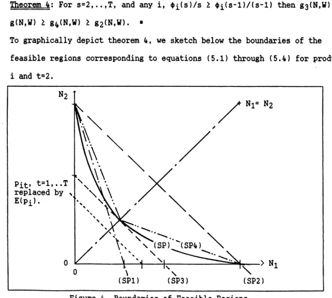
ThLg.rem 4: For s=2,..,T, and any i, i(s)/s > i(s-l)/(s-l) then g3(N,W)
g(N,W) g(N,W) g2(N,W).
To graphically depict theorem , we sketch below the boundaries of the feasible regions corresponding to equations (5.1) through (5.4) for product i and t=2.
Figure 4. Boundaries of Feasible Regions.
The assumptions, for any i, i(s)/s 2 i(s-l)/(s-l), for s=2,..,T, and i(l) E(pi) are not unreasonable for most pdfs when (l-a) is small.
N2 Pit, t=l,..T replaced by E(Pi). N2 N1 (SPi) (SP3) (SP2) I i I
The first says that the (1-a) fractile of the sum of random variables after scaling for the number of terms gets larger with more terms in the sum. Plainly, it means that the risk of getting very low yield rates is less when a given production quantity is divided into more lots. This is carried
forward from the conventional wisdom of not putting all the eggs in one basket. The second assumption says that the (1-a) fractile of a random
variable is less than its expected value.
Theorem 5 [Relative Error Bounds]: Let (N*,W*) be the optimal solution to the deterministic approximation (DPk) under consideration. For each k, the relative error of the value of this solution to the value of the optimal solution to (SPk) is bounded above by (ZUk(N*,W*) - ZDPk)/ZDPk where ZUk(N,W) is the value of any feasible solution (N,W) in (SPk).
Proof: By definition of (N*,W*),
ZDPk = h Eni=l.Tt=l(EtT=l(E(qi)N* + kea(i)WkiT* - Zjeb(i)Wiji - din)) + c Tt=l Nt*. (N*,W*) optimal to (DPk) implies that it is feasible in (SPk), ZSPk < E{h .ni=1ETt=1(.tT=1(qiN,* + Ekea(i)Wki* - jeb(i)Wij* - din))+ + c Tt=1 Nt*} - ZUk(N*,W*). Note that (t=l(qizNT + kea(i)WkiT
-Ejeb(i)Wijt - diT))+ is convex in (t,=lqiNU). Therefore by Jensen's inequality, for any (N,W),
E{h.ni=jlTt=l(Et=l(qiN + Ekea(i)Wki - jeb(i)Wij - din))++ cTt=l Nt)
hni=1ZTt=l(t=l(E(qi)N + kea(i)Wki - Eieb(i)Wij - din))++ cTt=lNt.
The optimal value of the left-hand side over Gk leads to ZSPk > ZDP+k and hence ZUk(N*,W ) ZSPk ZDP+k ZDPk. The relative error,
REk = (ZSpk - ZDPk)/ZSPk (ZUk(N*,W*) - ZDPk)/ZDPk.
5. Heuristics
So far we have examined the problem with plans frozen for the whole planning horizon. We believe these plans can be improved if they are
adapted to new available information. One way of adapting is to use a rolling planning horizon. In this section, we solve linear programs (DP2),
(DP3), and (DP4) to provide plans for the current period using demand
information for a given horizon. We denote these as SP2, SP3, and RH-SP4 respectively. (DP1) was not considered because of the non-uniformity of its feasible region vis-a-vis (SP).
We next generate heuristics based on the analytical results obtained earlier. The motivation for doing this is to examine how well these simple rules derived from theoretical results can perform. If the heuristics are good, they become practical alternatives for solving the problem without relying on extensive computational power. In our heuristics, the
downgrading quantities will not be computed directly. To ensure that units which have alternative uses are not double counted, we need to extend the definition of aggregates. We define the expanded aggregate i, AE(i) as equal to {i} if a(i) is empty, and {k:keAE(j),jea(i) U
(k:a(k)eAE(j),jea(i), otherwise. Some of the sets AE(.) may be the same. We can eliminate the redundant ones and keep only those that are distinct. The distinct AE(.) sets can be constructed using a Breadth-First Search. We redefine the sets AE(.) as AU(i), i=n+l,... . From now on we refer only to this extended set AU(i), i=1,..,2n. Depending on the product substitution structure, for n products, we can now have from n to 2n aggregates.
Two classes of heuristics were examined: heuristics with and without inventory withholding rules. We introduce three new heuristics that do not withhold inventory. In the first of these heuristics, U1, the production quantity decision mimics the deterministic approximations with one period planning horizon. (The problems (DPk) for k=l,.. , are indistinguishable when T=i.) For each aggregate i, we find the smallest Ni that needed to
satisfy the net demand (demand less inventory plus backorders) of the aggregate. We then set the production quantity as the largest of the Nis. Product demands are met directly from the inventory of their corresponding items when possible. We examine for shortages of products in ascending order of their labels. When shortage occurs, we downgrade from their
immediate predecessors in the product substitution structure, also in order of their labels, and work up the hierarchy till the shortage is resolved or no more inventory for downgrading is available. We list below the algorithm of heuristic U1 for the serial product substitution structure.
Hguristic U1
a. LET Dil = Dil - Iio, for all i.
b. LET Ni = Dil*/@i(1), for all i.
N* = Maxi { 0, Ni ), the production quantity.
c. [The item yields qi are realized.] Update inventory after direct assignment, Jil = qiN* + Jio - dill, for all i.
d. Downgrading:
FOR i=l to n AND IF Jil <
FOR j=i-1 to 1 step -1 AND IF Jjl > 0 Downgrade from i to i till
i) Jil = 0 or ii) Jjl = 0 NEXT i,i. a
The next two heuristics examine the demand of two periods and assume that the production of the next period will be the same as that of the current period. U2-SP3 mimics (DP3) and U2-SP2 mimics (DP2). The
downgrading rules are as in U1. Part b of U is modified as follows for these two heuristics:
Heuristic U2-SP3
b. LET Nil = Di1*/%i(1), for all i.
LET Ni2 = (Dil* + Di2)/0i(2), for all i.
Heuristic U2-SP2
b. LET Nil = Dil*/Oi(1), for all i.
LET Ni2 = ((Dil* + Di2)/*i(1))/2, for all i.
N* = Maxi 0, Nil, Ni2 , the production quantity.
The second class of heuristics holds back, under a given rule, inventory of higher order items from satisfying the demand of lower order products. The rule rations scarce higher order items so as to conserve
them. This corresponds to trading-off the shortage cost of lower order items against the cost of producing more later to meet the demand of higher order items. For heuristics V, UWH01, and UWH02, the decision rule for the production quantity is the same as in Ul. V is the heuristic in Bitran and Dasu [1989]. The withholding rule in this heuristic keeps, for each
downgrading source, the net product demand relative to the total demand less than or equal to its corresponding item's (1-a) fractile. Heuristics UWHO1 and UWH02 are refinements of V. These two heuristics compare the
relative net demands of product pairs against the ratio of their items' (1-a) fractiles. We list only the changes for each of the heuristics as
follows: Heuristic V
c. (append to end of c.)
LET Di2*+ = Max (0, D(i-l),2*+ + di,2 - Jil), for i=l,..,n where
DO 2*+ = 0.
d. (replace box by)
Downgrade from i to i till
i) Jil = 0 or ii) IF Dn2*+ > 0 THEN
Dj2*+/Dn2*+ j (1l)
Update Dk2*+, k =1,..,n ENDIF
Heuristic UWH01
c. (append to end of c.)
LET Di2*+ = Max (0, D(i-1),2*+ + di,2 Jil) for i=l,..,n where D2 + = 0.
d. (replace box by)
Heuristic UWH02
c. (append to end of c.)
LET Di2*+ = Max (0, D(i-l),2*+ + di,2 - Jil), for i=l,..,n where D0,2*+= 0.
d. (replace box by)
6. Computational Results and Comments
The heuristics were tested on thirty test cases, each with three products having a serial substitution structure. The expected yields and the coefficients of variation of the items relative to each other were
selected so that they cover a wide variety of possible combinations. The details of the test cases are found in the appendix. We simulated the application of the heuristics for 1000 periods.
Downgrade from i to i till
i) Jil = or ii) IF Dn2*+ > O THEN
Dj2*+/Dn2*+ < j(1)/n(1) Update Dk2 +, k =l,..,n ENDIF
Downgrade from i to items k=j+l to i in that order of priority till
i) Jil = 0 or ii) IF Dn2 > O THEN
Dj2*+/Di2*+ < j(1)/i(l) Update Dk2*+, k =l,..,n ENDTF
During the simulation, we calculate the average total cost per period, mean and standard deviation of production quantities per period, service levels, and statistics on inventory positions at the end of each period. Simulations for a fixed planning horizon were also done to 10 test cases randomly selected from the previous 30. Each of these was simulated for 4 periods planning horizon 1000 times. The plan was applied each time as if it was frozen for 4 periods. The upper bound on the relative errors of the deterministic approximation for the stochastic approximation are
obtained using theorem 5. RESUL
The simulations demonstrated that the deterministic approximations under the rolling horizon perform very well. They all meet service
requirements. RH-SP4 was found to perform the best. Among the LPs, RH-SP4 has the lowest average per period cost in 19 out of the 30 cases. RH-SP2 and RH-SP3 did not differ from each other at all in their performance. On the whole, RH-SP4 is 6.98% lower in cost than RH-SP3. In the best case it is 49.49% cheaper, at its worst it is 16.62% more expensive. Table 1
presents the results above. The static simulations showed that the average upper bound on the relative error of approximating (SP4) with (DP4) is about 3%.
Table 1 - Ls under Rolling horizon
(Out of 30 test cases; comparing among R-Hs.)
Average % Average % (Max.+ %) (Max.+ %) [Max - %] [Max - %] No. of Average % Maximum % Deviation Deviation
Times Deviation Deviation From From
Methods Best From Best From Best RH-SP3 RH-SP4
RH-SP/ 19 2.17 16.62 -6.98 0.00 (16.62) (0.00) [-%9.49] [0.00] RH-SP3 11 14.57 97.99 0.00 12.36 (0.00) (97.99) [0.00] [-14.25] RH-SP2 --- SAME AS RH-SP3 ---Note: Negative indicates the method is better.
From the results of the simulation, it seems advisable not to
withhold inventory. The withholding of higher order items was motivated by the argument that it may be cost effective not to downgrade scarce high order items since the higher order items are relatively more difficult to produce. However, not downgrading items degrades the service performance of the lower order products. The relative scarcity of higher order items imply that the lower order items are in relative abundance. The service
performance of the products corresponding .to these low order items are then usually good, so withholding may not cause the service targets of these products to be violated. But if this is so, then the frequency of requests for downgrading will be so small that the additional cost incurred by downgrading, when it is needed, is negligible. Hence, it is reasonable not to restrict downgrading. This conclusion is consistent with the results in Table 2.
Table 2 - All Heuristics
(Out of 30 test cases; comparing among heuristics.)
No. of When service limits
Times are violated:
No. of- No. of Violated Average Worst
Times Times Service Service Service
Methods Best Second Limits Level Level
U1 7 9 0 - -U2-SP3 10 14 0 -U2-SP2 12 6 0 - -V 7 5 12 54.93 96.00 UWHO1 6 5 12 48.88 96.30 UWH02 6 5 9 48.43 36.70
Note: Best heuristics must have the lowest average per period cost as well as satisfy service limits. The number of 'best' exceeds 30 because of ties.
The main reason against using withholding heuristics is that they do not guarantee meeting service targets. Shortage probabilities for cases under withholding heuristics can be extremely high. For some of the test cases, simulation shows that under these heuristics, service requirements are violated in as many as 12 out of the 30 test cases. The average
shortage probabilities among the violation cases range from 25.50% to 48.43% with the maximum service performance failing to meet demand 96.30% of the periods. The withholding heuristics do not differ very much from
each other. Table 2 above presents more details.
As a whole, a myopic rule like U was found to do well. In fact, Ul's performance was the same as RH-SP3 and RH-SP2. It appears then that, unlike RH-SP4 which was able to make use of future periods' information within its
plan, RH-SP2 and RH-SP3, though both also multi-period formulations, were not able to exploit that. This does indicate that planning beyond one period is beneficial. We postulate that it will be more so when there are capacity constraints and seasonality in demand. Counting only cases that do not violate service constraints, U1 performs better than any of the other
For the 'two period' heuristics, U2-SP2 is the best heuristic in 12 out of the 30 cases. This is almost twice as many times as compared to the
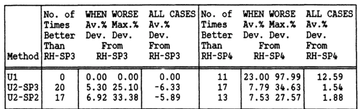
'one period' rules. U2-SP3, the other 'two period' rule, performed just as well with 10 firsts and 14 seconds. We now compare U1, U2-SP3 and U2-SP2 against RH-SP4, the best method. Looking at Table 3 below, it is easy to see that U1 is on the average 12.59% higher in cost than RH-SP4. U2-SP3 and U2-SP2 both perform much better with average relative deviation in cost from SP4 of less than 2%. They also do better than the best method, RH-SP4, in about half of the test cases. We can conclude that the 'two-period' heuristics are much better than the 'one-period' heuristics. Also, the two
'two-period' heuristics though based on very simple rules, did almost as well as the computationally more intensive RH-SP, a 4 period LP under rolling horizon.
Table 3 - Service Conforming Heuristics Relative to RH-SP3 and RH-SP. (Out of 30 test cases)
No. of WHEN WORSE ALL CASES No. of WHEN WORSE ALL CASES
Times Av.% Max.% Av.% Times Av.% Max.% Av.%
Better Dev. Dev. Dev. Better Dev. Dev. Dev.
Than From From Than From From
Method RH-SP3 RH-SP3 RH-SP3 RH-SP4 RH-SP4 RH-SP4
U1 0 0.00 0.00 0.00 11 23.00 97.99 12.59
U2-SP3 20 5.30 25.10 -6.33 17 7.79 34.63 1.54
U2-SP2 17 6.92 33.38 -5.89 13 7.53 27.57 1.88
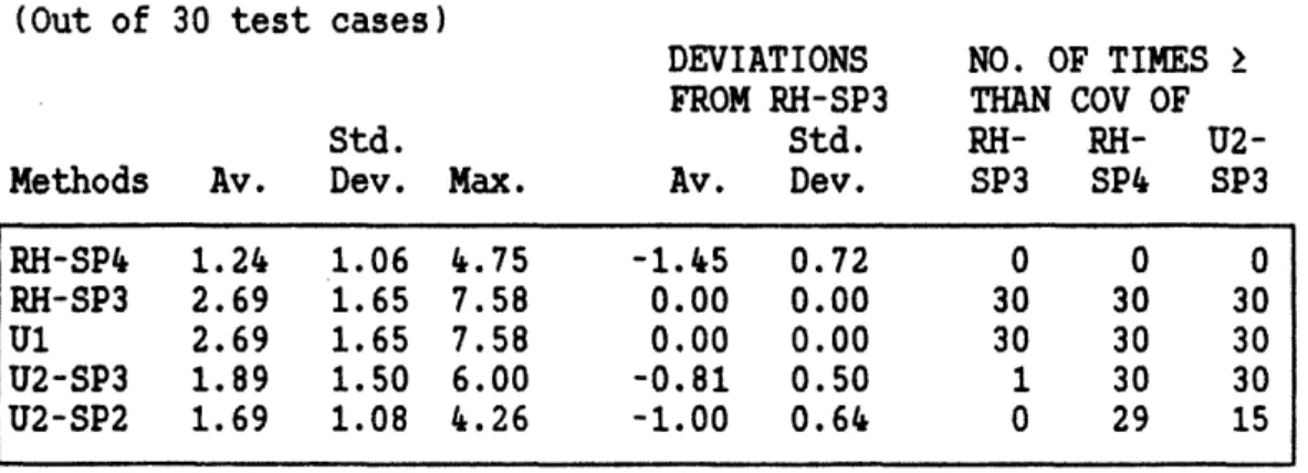
Another interesting result is that the coefficients of variation (COV) of production quantity of the better methods are also lower. RH-SP4's COVs are smaller than the COVs of SP3 and SP2. In turn SP3 and U2-SP2's COV are much smaller than those of RH-SP2 and RH-SP3. In 20 out of the 30 cases, the RH-SP4's COVs are less than one half than that of RH-SP3. The average COVs are 2.69, 1.24, 2.69, 2.69, 1.89, and 1.69 for SP3,
RH-SP4, RH-SP2, U1, U2-SP3, and U2-SP2 respectively. Table 4 below present the results.
Table 4 - Coefficient of Variation of Production Quantitfes
(Out of 30 test cases)
DEVIATIONS NO. OF TIMES
FROM RH-SP3 THAN COV OF
Std. Std. RH- RH-
U2-Methods Av. Dev. Max. Av. Dev. SP3 SP4 SP3
RH-SP4 1.24 1.06 4.75 -1.45 0.72 0 0 0 RH-SP3 2.69 1.65 7.58 0.00 0.00 30 30 30 U1 2.69 1.65 7.58 0.00 0.00 30 30 30 U2-SP3 1.89 1.50 6.00 -0.81 0.50 1 30 30 U2-SP2 1.69 1.08 4.26 -1.00 0.64 0 29 15 GENERAL COMMENTS
Linear deterministic equivalents are useful and practical because sensitivity analysis can be done 4t no additional computational effort. This makes it easy to evaluate the cost of meeting the service
requirements. Interactive-type approaches may be incorporated for adjusting the service requirements to trade-off the cost and value of the service constraints. Nonlinear deterministic equivalents and other linear
deterministic equivalents have been suggested for chance-constrained
problems. (See Hillier [1967], and Seppala [1971].) These usually assume a particular type of pdf for the random variables. The assumption is not restrictive in most cases but does not hold for distributions that have
fixed supports. Therefore, formulating the deterministic nonlinear program equivalent of our problem is already a big challenge. Also in problems where there is a large number of other linear constraints (other than those we generate to replace each chance constraint; for example, multiple
resources production capacity constraints) nonlinear programming approaches become very inefficient.
Our approach is an inner linearization method. Unlike other inner linearization methods, we do not need the functions to be separable. Outer linearization approaches are usually used when nonlinear programming
methods are employed. The solution to an outer linearization approximation of the problem is uniformly looser and hence may be infeasible. The gap from feasibility may be small when there are many linearization "cuts" and as mentioned in Hillier [1967], they are "barely infeasible". The outer linearization methods are often multi-pass techniques. Our method, as presented in this paper, solves for a planning horizon in one pass.
(DP4) is a simple version of a class of deterministic linear programs that can closely approximate the chance-constrained problem (SP). More advance, near-optimal single-pass as well as multi-pass linear programs can be constructed to approximate and solve (SP) by clever selection of rays in the construction of (SP4). We have used (SP6) in its current form for our problem and found that it is significantly better than the more common (SP2)-type approach. (For example, see Olson, and Swenseth [1988] and Allen, Braswell, and Rao [1976].) Our approach in this paper, increased the total number of constraints needed in our test cases from 2 (for SP2 or SP3) to 51 (for SP6).
It is interesting to note that, RH-SP4, a rolling horizon
implementation of (DP6) can perform so well in a dynamic situation. Even more remarkable is that U2-SP3, a simple heuristic motivated by (DP3), differs only slightly in performance from the more sophisticated and computational more intensive RH-SP4. (U2-SP3 can also be called U2-SP4 since assuming N1 = N2 makes the second period constraints in (SP3) and
In our computations, we have used fractiles obtained by Monte-Carlo simulations since no closed-form expression for them exists. In practice, sometimes the form as well as the values of the parameters of the joint yield distributions are not known. Historical data may be limited. In such
situations, the data may be used to construct distribution-free (1-a) fractiles. When the form of the distribution is known, approaches similar to those in Bache [1979] using results of Cornish, and Fisher [1937] and Fisher, and Cornish [1960] may be used.
In this paper, we have assumed the capacity is unrestricted and costs constants are time-invariant. The reader will notice that these can be relaxed for the LP formulations. Heuristics can also be derived for the capacitated situation though this will require additional work. The derivation of these heuristics and evaluation of their performances, and the relaxation of other assumptions like the transitivity of substitution remain topics for future research.
7. Summary and Conclusions
We provided LP formulations that approximate the original problem with uniformly tighter constraints and computed, for each approximation, the corresponding optimal production plan. The uniformly tighter feature is
important if planning is done infrequently since the production plan must satisfy the service constraints for the planning horizon. When planning is done every period, the approaches in this paper provide feasible solutions even under conditions of demand seasonality and capacity constraints. Our models rely on the benefit of solving problems with more than two periods. This characteristic is particularly useful when the plans are determined on
a rolling horizon basis since they tend to change less nervously from period to period.
Acknowledgements
The authors are grateful to Prof. Devanath Tirupati and Mr. Steve Gilbert for their comments on an earlier version of this paper.
REFERENCES
ALLEN, F.M., R. BRASWELL and P. RAO 1974. "Distribution-free Approximations for Chance-Constraints," Op. Res. 22, 610-621.
BACHE, N. 1979. "Approximate Percentage Points for the Distribution of a Product of Independent Positive Random Variables," Appl. Statist. 28, 158-162.
BITRAN, G.R., and H.H. YANASSE 1986. "Deterministic approximations to stochastic production problems," Op. Res. 32, 999-1018.
BITRAN, G.R., and S. DASU 1989. "Order Policies in an Environment of
Stochastic Yields and Substitutable Demands," Working paper t3019-89-MS, Sloan School of Management.
CHARNES, A., and W.W. COOPER 1963. "Deterministic Equivalents for
Optimizing and Satisficing under Chance Constraints," Op. Res. 11, 18-39.
CORNISH, E.A. and R.A. FISHER 1937. "Moments and cumulants in the
specification of distributions," Rev. Int. Statist. Inst. 5, 307-321. DEUERMEYER, B.L., and W.P. PIERSKALLA 1978. "A By-Product Production System
with an Alternative," Mgmt. Sci. 24, 1373-1383.
FISHER, R.A. and E.A. CORNISH 1960. "The percentile points of distributions having known cumulants," Technowetrics 2, 209-225.
GERCHAK, Y., R.G. VICKSON, and M. PARLAR 1988. "Periodic Review Production Models with Variable Yield and Uncertain Demand," IIE Trans. 20, 14-150.
HENIG, M. and Y. GERCHAK 1989. "The Structure of Periodic Review Policies in the Presence of Random Yield," forthcoming in Op. Res.
HILLIER, F.S. 1967. "Chance-constrained programming with 0-1 or bounded continuous decision variables," Mgmt. Sci. 14, 34-57.
KARMARKAR, U. 1987. "The multilocation multiperiod inventory problem: bounds and approximations," Mgmt. Sci. 33, 86-94.
KARMARKAR, U. and S-C. LIN 1987. "Production Planning with Uncertain Yields and Demands," Working paper, Simon Graduate School of Business
LEE, H.L., and C.A. YANO 1988. "Production control in multi-stage systems with variable yield losses," Op. Res. 36, 269-278.
LEE, H.L., and C.A. YANO 1989. "Lot-Sizing with Random Yields: A Review," Technical Report 89-16, Dept. of Industrial and Operations Engineering, U. of Michigan.
LEVY, L.L. and A.H. MOORE 1967. "A Monte-Carlo technique for obtaining system reliability confidence limits from component test data," IEEE trans. Rel. R-16, 69-72.
MAZZALO, J.B., W.F. McCOY, and H.M. WAGNER 1987. "Algorithms and heuristics for variable-yield lot sizing," Nav. Res. Log 3, 67-86.
McGRILLIVRAY, A.R., and E.A. SILVER 1978. "Some concepts for inventory control under substitutable demand," INFOR 16, 67-63.
MOINZADEH, K. and H.L. LEE 1987. "A Continuous Review Inventory model with constant resupply time and defective items," Nav. Res. Log 34, 457-468. OLSON, D.L. and S.R. SWENSETH 1988. "A Linear Approximation for
Chance-Constrained Programming," J. Opl. Res. Soc. 38, 261-267.
PARLAR, M. and S.K. GOYAL 1984. "Optimal ordering decisions for two substitutable products with stochastic demands," Opsearch 21(1). SEPPALA, Y. 1971. "Constructing Sets of Uniformly Tighter Linear
approximations for a Chance Constraint," Mgmt. Sci. 17, 736-749. SHIH, W. 1980. "Optimal Inventory Policies when stockout results from
Defective Products," Int'l J. Prod. Res. 18, 677-686.
SILVER, E.A. 1976. "Establishing the Reorder Quantity when the Amount Received is Uncertain," INFOR 14, 32-39.
APPENDIX Test Cases
There are thirty test cases, each with three products 1, 2, and 3. Related to these products are 4 items, one for each product and the fourth for the rejects. The substitution structure is serial and transitive. That
is, item 1 can be used as products 1, 2, or 3; item 2 can be used as products 2 or 3; and item 3 can only be used as product 3. The mean yield rate of each of the first three items in each problem is set L(ow),
M(edium), or H(igh) relative to each other. The approximate values for L, M, and H yield rates are 0.1, 0.3, and 0.5 respectively.
We define yield rate of con-aggregate i (short for conditional
aggregate) as the ratio of the sum of the yield rates of items deliverable as product i to the sum of the yield rates of items deliverable as product (i+1), for i=1, 2, 3. The coefficient of variation of each con-aggregate
(CCV) is also set L, M, or H relative to each other. The con-aggregates are assumed to have Beta distributions. This is a common distribution for
random variables that range between 0 and 1 and is general enough to approximate most empirical yield distributions. The (1-a) fractiles are generated by Monte-Carlo simulations. The test cases are set up with the parameters a and b for the distribution roughly according to the
specifications outlined for each case. These cases are listed in the table below:
Each box above contains the parameters for one test case. The total demand of all three products in each period is assumed to be uniformly distributed between 750 and 1250 units, with a mean of 1000 and a range of
500. The total demand is assigned to the 3 products according to the ratios of 3 randomly generated numbers. Unit production and holding costs are 8 and 1 respectively and a is set at 0.95.
CCV MEAN LMH LHL MMM MLM HML Items a b a b a b a b a b LMH 1 22 177 21 128 82 164 116 155 177 142 2 6 7 11 2 5 3 4 3 13 2 3 9 1 2 1 5 1 1 1 5 1 LHL 1 22 177 21 128 82 164 116 155 177 142 2 1 1 3 1 1 1 1 1 4 1 3 110 12 119 51 110 12 187 80 110 12 MMM 1 2 19 3 20 2 5 3 4 4 3 2 6 7 11 2 5 3 4 3 13 2 3 27 3 7 3 15 2 5 2 15 2 MLM 1 2 19 3 20 2 5 3 4 X 3 2 86 108 158 26 133 66 171 128 123 15 3 27 3 7 3 15 2 5 2 15 2 HML 1 1 6 1 3 1 1 1 1 1 1 2 6 7 11 2 5 3 4 3 13 2 3 110 12 119 51 110 12 187 80 110 12 HHH 1 1 4 1 1 3 1 1 1 1 1 2 1 1 3 1 1 1 1 1 4 1 3 5 1 1 1 5 1 1 1 5 1
M.I.T.Sloan School of Management Working Paper Series Papers by Gabriel R. Bitran
Nippon Telegraph and Telephone Professor of Management Science
Paper # Date TitlelAuthor(s)
3115 1/90 "Analysis of Phi / PH / 1 Queues," Bitran, G.R., and Dasu, S.
3111 1/90 "Distribution-Free, Uniformly-Tighter Linear Approximations for
Chance-Constrained Programming," Bitran, G., and Leong, T.
3108 12/89 "Hotel Sales and Reservations Planning," Bitran, G., and Leong, T.
3097 11/89 "Co-Production of Substitutable Products," Bitran, G., and Leong,
T.Y.
3090 11/89 "Ordering Policies in an Environment of Stochastic Yields and
Substitutable Demands," Bitran, G., Dasu, S.
3071 8/89 "Deterministic Approximations to Co-Production Problems with
Service Constraints" Bitran, G., and Leong, T.
3054 "Sequencing Production on Parallel Machines with Two Magnitudes
of Sequence Dependent Setup Costs," Bitran, G., and Gilbert, S.
3019 "Ordering Policies in an Environmnent of Stochastic Yields and
Substitutable Demands," Bitran, G., and Dasu, S.
3017 "Hierarchical Production Planning," Bitran, G., and Tirupati, D.
2519 3/89 "Approximation for Manufacturing Networks of Queues and
Overtime," Bitran, G., and Tirupati, D.
1744 2/86 "Planning and Scheduling for Epitaxial Wafer Production
Facilities," Bitran, G., and Tirupati, D.
1764 3/86 "Multiproduct Queueing Networks with Deterministic Routing:
Decomposition Approach and the Notion of Interference," Bitran, G., and Tirupati, D.
1635 3/85 "An Optimization Approach to the Kanban System," Bitran, G.,
and Chang, L.
1486 10/83 "Introduction to Multi-Plant MRP," Bitran, G., Marieni, D., and
Noonan, J.
1402 2/83 "A Simulation Model for Job Shop Scheduling," Bitran, G., Dada,
M., and Sison, L.
1391 1/83 "Productivity Measurement at the Micro Level," Bitran, G., and
Paper # Date Title/Author(s)
1282 2/82 "Analysis of the Uncapacitated Dynamic Lot Size Problem,"
Bitran, G.R., Magnanti, T.L., and Yanasse, H.H.
1271 11/81 "Computational Complexity of the Capacitated Lot Size
Problem," Bitran, G.R., and Yanasse, H.H.
1272 10/81 "Diagnostic Analysis of Inventory Systems: A Statistical
Approach," Bitran, G.R., Hax, A.C., and Valor-Sabatier, J.