Towards improved source apportionment of anthropogenic methane sources

(1)

HAL Id: tel-01760131

https://tel.archives-ouvertes.fr/tel-01760131

Submitted on 6 Apr 2018

HAL is a multi-disciplinary open access archive for the deposit and dissemination of sci-entific research documents, whether they are pub-lished or not. The documents may come from teaching and research institutions in France or abroad, or from public or private research centers.

L’archive ouverte pluridisciplinaire HAL, est destinée au dépôt et à la diffusion de documents scientifiques de niveau recherche, publiés ou non, émanant des établissements d’enseignement et de recherche français ou étrangers, des laboratoires publics ou privés.

Towards improved source apportionment of

anthropogenic methane sources

Sabina Assan

To cite this version:

Sabina Assan. Towards improved source apportionment of anthropogenic methane sources. Earth Sciences. Université Paris Saclay (COmUE), 2017. English. �NNT : 2017SACLV079�. �tel-01760131�

(2)

Towards improved source

apportionment of anthropogenic

methane sources

Thèse de doctorat de l'Université Paris-Saclay

préparée à Université de Versailles – Saint-Quentin-en-Yvelines

École doctorale n°129 Sciences de l'environnement d’Ile-de-France

(SEIF)

Spécialité de doctorat: chimie atmosphérique

Soutenance a Gif Sur Yvette, le 18th décembre 2017 .

Sabina Assan

Composition du Jury : Philippe Bousquet

Prof. Des Universites, UVSQ Président

Martina Schmidt

Charge de Recherche, Heidelberg University Rapporteur

Thomas Roeckmann

Professeur, Utrecht University Rapporteur

Nadine Locoge

Professeur, University of Lille Nord Examinateur

Philippe Ciais

Directeur de Recherche, LSCE Directeur de thèse

Valerie Gros

Directeur de Recherche, LSCE Co-Directeur de thèse

Felix Vogel

(3)

Title : Vers une répartition améliorée des sources de méthane anthropique

Keywords : méthane isotopes, COVs, CRDS

Le méthane a la deuxième plus grande contribution à au forçage radiatif global des gaz à effet de serre anthropiques. Après une période de stabilité, son taux de croissance atmosphérique a augmenté rapidement depuis 2007. Les émissions anthropiques de méthane ont un potentiel important d'atténuation ce qui encourage les efforts visant à réduire ses émissions conformément à l'accord de Paris. Toutefois, beaucoup d’incertitudes demeurent concernant la contribution de différentes sources de méthane, les processus et les estimations des émissions, même à une échelle locale ; ce qui entrave la mise en œuvre efficace des stratégies d'atténuation du méthane. Jusqu’à maintenant, de nombreuses études ont été réalisées pour mesurer les flux globaux de méthane, la répartition et la caractérisation des sources de méthane par région mais les processus doivent encore être mieux déterminés.

Cette thèse présente et applique des méthodes pour caractériser les différentes sources de CH4

présentes dans les mesures de l'air ambiant des sites industriels et développe des outils ciblés pour répondre à cette question. Le premier chapitre traite des améliorations apportées à un instrument CRDS fréquemment déployé pour les mesures de CH4 et de δ13CH4. Nous proposons un schéma

d'étalonnage pour corriger les interférences C2H6 sur δ13CH4 et permettre des mesures fiables de

C2H6. Les résultats de ces travaux sont ensuite utilisés pour explorer la valeur ajoutée sur les

données de la mise en œuvre de cette méthode sur une station de compresseur de gaz naturel, où une forte corrélation de C2H6 et de CH4 est normalement attendue. Le deuxième chapitre poursuit la

caractérisation des sources de CH4 sur le même site mais porte plus sur l'application et la

comparaison des différentes méthodes de répartition des sources. Les contributions des sources de CH4 et composés organiques volatils (COV) sont explorées selon la méthode de l'analyse isotopique,

(4)

3

PMF), des données météorologiques et des échantillons directs de gaz naturel. Le troisième chapitre présente une utilisation des méthodes de répartition des sources de CH4 sur les mesures ambiantes

des sources de CH4 biogénique dans la région Ile de France et aide ainsi à compléter l'étude des

sources anthropiques de CH4 les plus pertinentes.

Cette thèse identifie et documente les signatures en δ13_CH

4 de différentes sources de CH4 sur des

environnements contrastés à proximité de fermes d’élevage intensif, de stations d’épuration des eaux usées, de décharges d’enfouissement des déchets ou encore de sites de compression du gaz naturel, et étudie leur variabilité spatiale et temporelle pour faciliter la contrainte des émissions. Les résultats obtenus suggèrent que l’identification de différentes sources biogéniques et thermogéniques avec le δ13_CH

4 est robuste et adaptable à une grande diversité d’environnements.

L'utilisation d'une combinaison d'outils est idéale pour étudier la variabilité à court terme et long terme. Cette thèse présente différentes utilisations de ces nouveaux outils pour diriger les investigations des émissions anthropiques de méthane et sont la base pour de futurs travaux dans ce domaine.

(5)

Title :

Towards improved source apportionment of anthropogenic methane sources

Keywords : Methane isotopes, VOCs, CRDS

Methane has the second largest contribution to the global radiative forcing impact of anthropogenic greenhouse gasses. Since 2007 its atmospheric growth rate, after a period of stability, has again been rising rapidly. Anthropogenic methane emissions hold a large mitigation potential, promoting efforts to curb emissions in accordance with the Paris Agreement. However, the considerable uncertainties regarding methane contributors, drivers and emission estimates even at local scales, hinder the effective implementation of methane mitigation strategies. While many approaches have been established to measure total methane fluxes, the partitioning and characterisation of methane sources by region and processes still need to be better constrained.

This thesis presents practical methods for characterising different CH4 sources in ambient air

measurements at industrial sites, as well as developing more targeted tools. The first chapter focuses on improvements to a CRDS instrument that is commonly deployed for CH4 and δ13CH4 field

measurements. We propose a calibration scheme to correct for C2H6 interference on δ13CH4, and

enable robust C2H6 measurements. The results of this work are then used to explore the added value

gained when implemented on data from a natural gas compressor station, a site where high correlation of C2H6 and CH4 is expected. The second chapter continues the investigation of CH4

sources at the same site; with focus shifted towards the application and comparison of different source apportionment methods from time series analysis based on measurements of multiple species, some co-emitted with CH4. Here the CH4 and Volatile Organic Compounds (VOC) source

contributions are explored through the use of isotopic analysis, receptor model analysis (PCA and PMF), metrological data and direct samples of natural gas. The third chapter applies a selection of the developed CH4 source apportionment methods to ambient measurements at biogenic CH4 sites in

the Ile de France region and helps complete the survey of the most relevant anthropogenic CH4

sources.

This thesis identifies and reports local δ13_CH

4 source signatures for livestock, wastewater, landfill and

natural gas and studies their spatial and temporal variability to aid the constraint of emission inventories. Our findings suggest that source apportionment from δ13_CH

4 is robust, and adaptable to

the majority of sites. Using a combination of tools is ideal for more specific source determination and for an understanding of long and short term variability. The work presented in this thesis offers example applications of these new tools to directed investigations of anthropogenic methane emissions and lays the foundation for future work in this field.

(6)

5

A

CKNOWLEDGMENTS

Firstly, I would like to express my sincere gratitude to Philippe Ciais, Felix Vogel and Valerie Gros for supervising my PhD. Thanks Philippe for your motivation, immense knowledge and constant new ideas of how to take the work forward. Thank you Felix for your continuous support, patience, and all the time you spent explaining, thinking and solving problems with me. Thanks also for all the hard work you put into this PhD, without which it would not be the finished product it is today. I could not have imagined a better advisor and mentor. Thank you Valerie for having followed my PhD, for all your advice, and for always being there when I needed help.

I would like to again thank Nadine Locoge, Thomas Roeckmann, Philippe Bousquet, and Martina Schmidt for accepting to be part of my PhD jury. Thank you also to Rod Robinson, Dave Lowry, and Gabrielle Petron for spending the time to take part in my PhD Committees throughout the years. Your constructive advice helped me to advance the work, and see ideas from a different perspective. Specifically thank you to Rod for your time and advice during field campaigns.

Thank you to Climate-KIC for financing this PhD. A big thank you also to Doug Worthy for welcoming me during my mobility to ECCC, and all the others I met during this exchange.

Thank you equally to Alexia Baudic, Sebastien Ars and Sandy Bsaibes for working with me and helping me throughout the different measurement campaigns. I would also like to say a big thank you to Ali Guemri, Dominique Baisnee and Olivier Laurent for all their technical help and lab measurements throughout the three years. Of course also a big thank you to everyone I met and worked with during my time at LSCE. A particularly massive thank you to Abdel, Xin, Lamia and Jens for all the good times we had, and for keeping me motivated and smiling throughout. It wouldn’t have been the same without you.

Finally I thank my friends and coloc-family who always encouraged me and made coming home after work a pleasure every evening.

(7)

Figures

Figure 1.1 AMAP Assessment 2015: Methane as an Artic climate forcer. _________________________________ 14 Figure 1.2 Inventories and emissions factors consistently underestimate actual measured CH4 emissions across

scales. Ratios > 1 indicate measured emissions are larger than expected from EFs or inventories. The main graph compares results to the EF or inventory estimate chosen by each study author. The inset compares results to regionally scaled common denominator, scaled to region of study and the sector under examinations. [Brandt et al., 2014]. ______________________________________________________________________________________ 16 Figure 1.3 Methane global emissions from 5 broad categories _________________________________________ 19 Figure 1.4 Genetic characterisation of natural gases by compositional and isotopic variations taken from Schoell (1983). _____________________________________________________________________________________ 23 Figure 2.1 Flow chart illustrating the steps involved to calibrate C2H6, and δ13CH4. _________________________ 31

Figure 2.2 Experimental Set-up. The dilution and working gas are connected via two MFCs to two CRDS instruments in parallel. In red is the placement of an optional glass flask used for the C2H6 calibration only. The flow is greater

than that of the instruments inlets, therefore an open split is included to vent additional gas and retain ambient pressure at the inlets. __________________________________________________________________________ 32 Figure 2.3 An example of the results from a H2O interference experiment spanning the range 0-1% H2O. _______ 38

Figure 2.4 The discontinuity seen for instrument CFIDS 2072 ___________________________________________ 38 Figure 2.5 Relationship between reported C2H6 and concentration changes of CO2 for instrument CFIDS 2072 and

2067 at varying values of H2O ___________________________________________________________________ 39

Figure 2.6 Relationship between reported C2H6 and concentration changes of CH4 for both instrument _________ 40

Figure 2.7 (a): Ethane calibration ________________________________________________________________ 42 Figure 2.8 During a dilution sequence of ambient gas with C2H6, the CH4 _________________________________ 44

Figure 2.9 The effect of C2H6 on reported δ13CH4. ____________________________________________________ 44

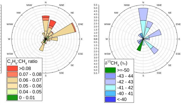
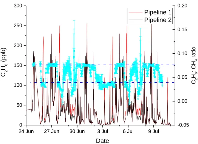
Figure 2.10 Ethane andMethane content of two selected peaks. _______________________________________ 51 Figure 2.11 Distribution of 16 events according to their C2H6: CH4 ratios and isotopic signature. _______________ 53

Figure 2.12 Flow chart illustrating the steps and the corresponding equations to calibrate C2H6 and δ13CH4 as

determined from this study. _____________________________________________________________________ 54 Figure 3.1 Aerial view of the natural gas compressor station and the location of the presumed principle natural gas sources _____________________________________________________________________________________ 59 Figure 3.2 Wind data plotted as a windrose for the period of the 25th of June 2014, to 3rd July 2014. ___________ 61 Figure 3.3 Monte Carlo simulation of Miller-Tans plots _______________________________________________ 62 Figure 3.4 Time series of 30min average concentrations of CH4, δ13CH4, CO2, VOCs and wind direction and speed

measured at the measurement campaign at the natural gas compressor station __________________________ 68 Figure 3.5 a) Pollution rose of mean CH4 concentrations plotted by wind speed and direction bins. ____________ 69

Figure 3.6 Temporal results plot. _________________________________________________________________ 72 Figure 3.7 Pollution-rose of the reconstructed C2H6:CH4 ratio of PC1 ____________________________________ 73

Figure 3.8 Modelled factors from the PMF analysis. __________________________________________________ 75 Figure 4.1 Arial image of Grignon farm and surrounding area. _________________________________________ 87 Figure 4-2 (Top) Fluctuation of the expected CH4 emissions (kg/d) estimated using IPCC Tier 1 method. (Bottom)

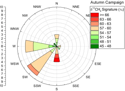
Weekly measurements of the live weight (metric tonnes) of each ruminant subgroup. ______________________ 90 Figure 4-3 Wind Rose _________________________________________________________________________ 91 Figure 4-4 Time series of mobile campaign at Grignon Farm. __________________________________________ 93 Figure 4-5 Methane source characterisation plot from mobile campaign at Grignon Farm. __________________ 95 Figure 4.7 (left) Methane excess rose at Grignon during the Autumn 2017 campaign. Y-axis signifies the count. (right) Polar plot of mean CH4 concentration with respect to wind speed and direction. _____________________ 99

(11)

Figure 4.6 Time series data of the variables measured during the Autumn 2017 measurement campaign at Grignon Farm. _____________________________________________________________________________________ 100 Figure 4.8 Isotopic Data from Autumn Campaign at Grignon. _________________________________________ 102 Figure 4.9 Isotopic signatures of CH4 concentration enhancements _____________________________________ 103

Figure 4.10 10h-mAPCA reconstructed ratios of the Principle Component calculated during the autumn campaign at Grignon Farm. X-axis is the time-series of CH4. Z-axis is: Top) C2H6:CH4 ratio. Bottom) CH4: CO2 ratio. Green dashed

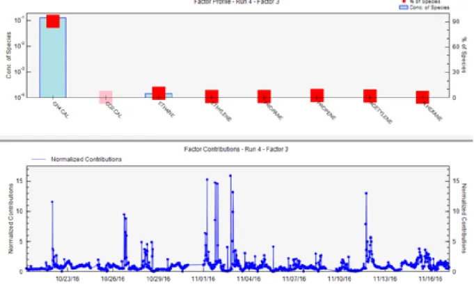
line signifies ruminant emissions measured during the mobile field campaign. ___________________________ 104 Figure 4.11 PMF results for autumn campaign at Grignon: Factor 2 profile [biogenic CH4 factor. Top) concentration

and percentage of species contributing to the factor. Bottom) temporal variation of normalised contributions of factor. _____________________________________________________________________________________ 105 Figure 4.12 (left) Methane pollution rose for spring campaign at Grignon _______________________________ 107 Figure 4.13 Temporal concentration data of the species measured during the spring measurement campaign __ 108 Figure 4.14 Isotopic data measured during the spring Grignon field campaign. ___________________________ 109 Figure 4.15 Variation of δ13CH4 signatures with respect to wind direction. X-axis represents count number. ____ 110

Figure 4.16 Temporal variation of (Top) Methane variability (Bottom) Reconstructed components modelled by MC-APCA. _____________________________________________________________________________________ 111 Figure 4.17 10h MC-mAPCA results for the spring campaign. Temporal variation of CH4 plotted in black on x-axis.

__________________________________________________________________________________________ 112 Figure 4.18 Factor 2 profile [CH4–only factor] ______________________________________________________ 114

Figure 4.19 Hourly, daily and weekly temporal variation of mean CH4 concentration for the spring and autumn

Grignon campaigns. __________________________________________________________________________ 115 Figure 4.20 Methane source characterisation plot. δ13CH4 signature on the y-axis and CH4: CO2 ratios on the x-axis.

Methane concentration peaks are plotted in dark and light blue for the spring and autumn campaign respectively. __________________________________________________________________________________________ 116 Figure 4.21 Comparison of δ13CH4 signatures from ruminants depending on their diet measured in this study and

literature __________________________________________________________________________________ 118 Figure 4.22 St Thibault–des-Vignes WWT site map. Inlet location is marked by a yellow star. ________________ 121 Figure 4.23 Wind rose from wind data at St Thibault WWT ___________________________________________ 122 Figure 4.24 Continuous observations of CH4, CO2, δ13CH4 and metrological data at St Thibault WWT plant during the

measurement campaign. ______________________________________________________________________ 124 Figure 4.26 Methane concentration roses for measurements by NPL at 13 locations surrounding the WWT facility. __________________________________________________________________________________________ 125 Figure 4.25 Methane concentration rose for measurements at inlet. Concentration in ppm. _________________ 125 Figure 4.27 Cergy Pointoise WWT site map _______________________________________________________ 126 Figure 4.28 Windrose for the duration of the Cergy-Pointoise WWT campaign ___________________________ 127 Figure 4.29 Continuous observations of CH4, CO2, δ13CH4 and metrological data at Cergy Pointoise WWT during the

measurement campaign. Green points are the periods for which isotopic signature was calculated. Blue points are periods for which both the isotopic signature and CH4:CO2 ratio was calculated. __________________________ 128

Figure 4.30 Mean CH4 concentrations (ppm) with respect to wind speed and direction. _____________________ 129

Figure 4.31 Isotopic signature with respect to wind direction _________________________________________ 130 Figure 4.32 Overview of experimental area of Buttes Bellot mobile measurement campaign. © Google Maps __ 132 Figure 4.33 Time-series of δ13CH4 measured downwind of the active landfill (Buttes –Bullot) using mobile

(12)

11

Tables

Table 1-1 An example of co-emitted VOCs that can be used as tracers to identify specific methane sources. ... 21

Table 1-2 Anthropogenic Methane sources and their indicative isotopic signatures ... 24

Table 1-3 Date, location, species measured and instrumentation used for the 6 measurement campaigns undertaken throughout the thesis. ... 25

Table 2-1 Description of the gas mixtures used to determine the cross sensitives of the interference of CH4, H20, CO2 on C2H6 and the interference of C2H6 on δ 13CH4. The respective ranges spanned during laboratory test, and the typical range at a natural gas site are noted on the right-hand side. ... 33

Table 2-2 Summary of C2H6 calibration factors calculated for both instruments CFIDS 2072 and 2067. ... 47

Table 2-3 The various response functions calculated for the δ13CH4 correction due to C2H6. ... 48

Table 3-1 Summary table specifying the implementation of the 3 identification methods used. ... 66

Table 3-2 Characteristics of gas taken from the two pipelines at the compressor station, from Assan et al. 2017. ... 67

Table 4-1 Results of source signatures from the mobile field campaign at Grignon Farm ... 95

Table 4-2 Weather conditions on 2.12.2016 ... 133

Table 5-1 Summary of isotopic source signatures for methane sources in Western Europe, and the values from this thesis. ... 139

(13)

Chapter 1 I

NTRODUCTION

1.1 T

HE ROLE OF

M

ETHANE IN GLOBAL WARMING AND CLIMATE CHANGE

The Earth’s climate system depends on the fine balance between incoming short wave and outgoing longwave solar radiation on the Earth’s atmosphere. Approximately half of the solar energy arriving at Earth, roughly 1370Wm-2, is absorbed by its surface, while about 30% is reflected back into space and 20% is absorbed in the atmosphere. The Earth’s surface in turn emits energy as longwave (infrared) radiation which is largely absorbed by a number of active gasses (H2O, CO2, CH4, N2O and other

greenhouse gases (GHG)). These re-emit the radiation in all directions; the downward component contributing to the heating of the lower layers of the atmosphere and thus increased global temperatures. As such, greenhouse gasses trap heat in the Earth’s atmosphere making them essential for life on earth. Since industrialisation (1750 onwards), global greenhouse gas concentrations within the atmosphere have been strongly increasing due to human activity, and are responsible for an additional radiative forcing of about 2.29Wm-2 [Myhre et al., 2013], thus disrupting the Earth’s radiative energy balance. In 1990, IPCC (Intergovernmental Panel on Climate Change) released its first major statement suggesting continued emissions of GHGs would likely result in global temperature and sea level rises. 25 years later, and the IPCC (and many research studies) have concluded that human activities have altered the Earth’s mean surface air temperatures over the last 100 years, and that climate change can lead to an increase in the occurrence and strength of extreme weather and climate events.

Being responsible for approximately 20% of all additional radiative forcing produced by GHGs so far, Methane (CH4) has been identified as one of the most important greenhouse gases. Anthropogenic

emissions are those resulting from human activities (IPCC Glossary of Terms) and currently account for 60% of all methane emissions. Predominant sources of anthropogenic emissions include: Agriculture (enteric fermentation and manure being the most important), fossil fuels, and waste decomposition. The impact of greenhouse gases is quantified by their Global Warming Potential (GWP) which is dependent on their radiative forcing and their residence time. Methane has a GWP 28-32 times that of CO2 on a 100-year time period and even greater on shorter timescales [Etminan, et al., 2016, Allen,

2014]. This is because CH4 is not only a potent GHG, but also reacts with OH radicals in the atmosphere

(14)

13

global warming. It does, however, have a relatively short lifetime (10 years [Patra et al., 2011]) in comparison to that of CO2 (50 to 200 years), thus making it an appealing gas to target for efficient, short

term climate change mitigation as emission reductions would yield short-term gains in radiative forcing.

1.2 T

HE

F

UTURE OF

M

ETHANE

Studies show that in recent years, unlike CO2, CH4 concentrations have been rising faster than at any

time in the past two decades, with a current atmospheric concentration 150% above pre-industrial levels (in 2016, the global annual mean is 1842.72 +/- 0.51 ppb [Dlugokencky, NOAA/ESRL]). Since 2007, the atmospheric methane growth has increased substantially (from 0.5 +/-3.1ppb per year for 2000-2006, to 6.9 +/- 2.7 ppb per year for 2007-2015 [Dlugokencky, 2016]), however, the relative methane contributors and drivers remain uncertain. Furthermore, annual anthropogenic CH4 emissions are

predicted to continue rising substantially; between 400 and 500Tg CH4 in 2030, and between 430 and

680Tg CH4 in 2050. The upper bar chart in Figure 1.1 shows the regional distribution of estimated annual

baseline CH4 emissions in 2030, by sector and world region in a continue as usual scenario. The

projected increase in emissions are greatest for methane from livestock and oil and gas systems as countries with fast growing economies and populations are expected to increase energy and waste consumption [EPA 430-R-12-006, 2012]. For example, China and Latin & Central America are expected to be the dominating emitters due to extensive coal, and cattle & oil industries respectively. These projected trends are in contradiction to the 2016 Paris Agreement wherein 195 countries adopted the action plan to limit the increase of global average temperatures to 1.5degC in order to reduce the risks and impacts of climate change. Given that anthropogenic methane emissions (responsible for over half of global methane emissions) are dominantly industry related suggests a large potential to reduce emissions. Studies suggest that at present, technically feasible mitigation methods hold the potential to prevent a third [USEPA, 2014] or half of future anthropogenic CH4 emissions by 2030 (reduction

potential of about 200 Tg CH4) [Hoglund-Isaksson, 2012]. Of this mitigation potential, more than 60%

can be realised in the fossil fuel industry from reduced venting and leakages. Thus, regions with the largest potential for CH4 mitigation are those with extensive fossil fuel extraction industries, in particular

China, Latin America and Asia (see Figure 1.1). Other large abatement potentials are the separation and treatment of biodegradable waste to replace landfills. As mitigation calculations from these studies are based strictly on technical abatement options, reductions from agricultural sources is limited due to the

(15)

requirement of changes in food production and consumption structures which are not deemed feasible on short timescale. To effectively create and implement CH4 mitigation methods, the sources and sinks

must be well characterised and understood. Unfortunately, up until now the sizes of fluxes from individual sources still remain highly uncertain.

1.3 U

NCERTAINTIES IN

M

ETHANE EMISSIONS ESTIMATES

For methane mitigation, it is vital to separate sources to aid planning purposes and green investment. Although methane emissions can now be inferred from inverse modelling as shown by recent studies [Pandey et al., 2016, Alexe et al., 2015, Hein et al., 1997], identifying and attributing contributions from multiple potential sources can be challenging. Hence emission inventories can aid to generate bottom up estimates of sector specific emissions which requires three steps: Identifying the sources of emissions, collecting the activity data and associated emission factors. Currently, existing bottom-up inventories do not well explain top down trends in methane emissions observed in the atmosphere

Figure 1.1 AMAP Assessment 2015: Methane as an Artic climate forcer.

Estimates of methane emissions in 2030 by world region from the GAINS model & maximum technically feasible reduction of methane emissions in 2030.

(16)

15

[Saunois et al., 2016, Hausmann et al, 2016, Kirschke et al. 2013, Nisbet et al 2014.]. Both methods have high uncertainties, as can be seen in the boxplots of Figure 1.3. For bottom-up estimates this may be because although generally sources are very well identified, emissions inventories still have very high uncertainties due to the uncertainties in individual source strength estimates. Brandt et al., (2014) find that inventories and emission factors consistently underestimate actual measured CH4 emissions in both

bottom-up and top-down studies, see Figure 1.2. The study is based on 20 years of literature on natural gas emissions in North America. Top down atmospheric studies (i.e. estimating CH4 emissions after

atmospheric mixing occurs) are plotted with a common baseline in the inset of Figure 1.2 which shows measured CH4 emissions are systematically higher than predicted by inventories. Results from device

and facility scale measurements (generally < 109 g CH4/year) are shown in the main chart of Figure 1.2.

While emissions factors were also found to underestimate the bottom up measurements, the results are more scattered than for atmospheric studies. Emission uncertainties are a consequence of the large variations seen in experimental data as emissions from anthropogenic sources can vary across space and time. Often inventories are based on single emissions factors for a given activity and/or from a small number of samples and point sources, e.g. IPCC Tier 1 methods, which do not sufficiently represent the areas and activities which they are applied to. For example, most studies on fugitive methane emissions from oil and gas are based on a limited number of studies specific to certain fields in the USA or Canada, however there are a number of parameters that will be country/site specific or change over time and thus without more systematic measurements their magnitudes will remain largely unknown for most major oil and gas producing countries. It is also possible that substantial sources remain outside of GHG emission inventories, for example abandoned oil & gas wells were found to contribute 5-8% of the estimated annual anthropogenic methane emissions for 2011 in Pennsylvania and are not included in the GHG emission inventory [Kang et al., 2016]. Thus, the requirement to improve current estimates means the partitioning of methane sources by region and processes need to be better constrained. To do this, observations of specific, individual methane sources must be extended.

(17)

Figure 1.2 Inventories and emissions factors consistently underestimate actual measured CH4 emissions across

scales. Ratios > 1 indicate measured emissions are larger than expected from EFs or inventories. The main graph compares results to the EF or inventory estimate chosen by each study author. The inset compares results to regionally scaled common denominator, scaled to region of study and the sector under examinations. [Brandt et al.,

(18)

17

1.4 A

NTHROPOGENIC

M

ETHANE

S

OURCE IDENTIFICATION

Besides dedicated emissions measurements, one important way to reduce uncertainties in methane inventories is by correctly distinguishing between emissions from various methane sources, often occurring in the same region. The formation of methane (either by biogenic, thermogenic or pyrogenic formation) dictates the individual characteristics of each methane source, e.g. their isotopic signature or species co-emitted, and as such an understanding of the processes involved in the creation of methane is particularly important.

1.4.1 M

ETHANE

F

ORMATION

Biologically produced methane arises through the decomposition of organic matter by methanogenic bacteria (archaea) under anaerobic conditions. The major anthropogenic sources arise from agriculture and waste. Agriculture, being the category with the largest contribution to anthropogenic CH4 releases

(approximately 45% [JRC/PBL, 2012]), has two predominant sources; rice paddies and livestock. Rice paddies, the lesser contributor between the two, mainly emit methane during the flooding period when the anaerobic conditions needed for methane production are present. Livestock emissions are estimated as double that of rice emissions globally, and are a result of the microbiological fermentation that breaks down cellulose and other macro molecules in the rumen [Lassey, K. 2006]. The produced CH4

and CO2 are released from the rumen mainly through the mouth of multi-stomached ruminants (87% of

ruminant emissions) [Saunois et al., 2016], generally cattle but can also be other domestic livestock such as sheep, goats, buffalo and camels. Emissions are strongly influenced by the total weight and diet of the animals. In addition, methane emissions arise when the livestock manure is stored or treated in systems that promote anaerobic conditions. The second biogenic category, waste, accounts for approximately 18% of total anthropogenic emissions [Saunois et al., 2016, Bogner et al. 2008] and includes two sub-sources, namely wastewater and landfill. Wastewater emissions occur when anaerobic conditions exist. This can be deliberately induced (specifically for wastewater with high organic content) or happen by coincidence [Andre et al. 2014]. In landfills, methane is produced as a waste gas due to the decomposition of organic material, and accounts for approximately 5-10% of global anthropogenic methane emissions [Bogner et al. 2008].

Thermogenic methane is typically produced during the decomposition of kerogen at depths below 1000m [Floodgate and Judd, 1991] at high temperature and pressures. In such conditions bacteria

(19)

cannot survive and the process takes place without any microbial activity leading to mature gases with higher CH4 concentrations. Its anthropogenic sources are predominantly fossil fuel methane emissions

(hereafter referred to as ffCH4), accounting for approximately 34% of global anthropogenic methane

emissions [Saunois et al., 2016]. Fossil fuel CH4 emissions arise from the production and use of Coal, Oil

and in particular, natural gas. Coal-related FFCH4, estimated between 8-12% of anthropogenic methane

emissions [Chai et al. 2016] is primarily emitted during the mining process when coal seams are fractured, but emissions can also occur during post mining processing such coal waste piles and abandoned mines [Penman et al., 2000 (IPCC)]. Natural gas is composed of >90% CH4, thus it is not

surprising that its loss to the atmosphere during extraction, processing and transport can represent a significant component of methane emissions. Natural gas is often co-located with petroleum, therefore, although on a lesser scale (in the US oil operations release one quarter as much CH4 as natural gas

systems), trapped methane is also released in large quantities during mining of petroleum (oil itself only contains trace amounts of methane so little is emitted during refinement/transportation [Smith et al., 2010]. It is estimated that emission factors for unconventional gas (gas trapped within shale formations mined via hydraulic fracturing) are larger than conventional oil and gas by 3-17%, due to higher releases in the drilling phase [Caulton, D. et al, 2014, Schneising et al., 2014, Howarth, 2011].

Finally, accounting for approximately 13% of anthropogenic emissions, pyrogenic methane arises from the incomplete combustion of biomass, thus the largest sources can be considered as peat fires, biomass burning and biofuel usage [Saunois et al., 2016]. The fraction of carbon that is released as methane depends on the fuel type and burning conditions, e.g. Burning dry savanna releases relatively small amounts of CH4 compared with forest fires [Encyclopedia of atmospheric sciences, Volume 3].

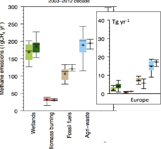
Estimates of global and European emissions from 5 broad methane source categories is shown in Figure 1.3, taken from the study Saunois et al. [2016]. Agriculture and waste emissions dominate in Europe.

(20)

19

1.4.2 VOC

E

MISSION

R

ATIOS

The formation of methane is often accompanied by a number of other compounds, whose abundances depend strongly on the creation conditions. Thus, it is possible to use correlations of co-emitted compounds with methane to distinguish between individual sources.

The term volatile organic compounds (VOCs) is used to denote the entire set of vapour phase atmospheric organics excluding CO and CO2. Given their short atmospheric lifetimes (fractions of a day

to weeks) they have little direct impact on radiative forcing but are central to atmospheric chemistry,

Figure 1.3 Methane global emissions from 5 broad categories (Wetlands, Biomass burning, Fossil fuels, and Agriculture and waste) for the 2003-2012 decade from top down inversion models (left light coloured

boxplots) and bottom up models/inventories (right, dark coloured boxplots) in Tg CH4yr-1 taken from

Saunois et al. 2016. The inset plots the regional CH4 budget for Europe using the same categories. In

Europe, anthropogenic methane (in particular Agriculture and Waste) are dominant over natural methane sources.

(21)

participating in atmospheric photochemical reactions and influencing the air quality and climate through their production of ozone and organic aerosols. Within this thesis, non-methane hydrocarbons (NMHC), which are organic chemical compounds consisting of hydrogen and carbon atoms emitted from both natural and anthropogenic sources are used as complementary tracers for CH4. Here, the words NMCHs

and VOCs are used interchangeably.

The majority of VOC emissions are related to natural sources which originate from nearly exclusively (approximately 90%) vegetation [Guenther et al., 1995]. Nonetheless, global emissions of anthropogenic VOCs is approximately 186 Tg/year [EDGAR 2005], of which a number of sources are shared with methane. The ratio of methane to light VOCs is very high for biologically produced methane because the biochemical mechanism for methanogensis are very specific, whereas in thermogenic reactions substantial amounts of ethane and propane can also be produced. VOCs can be separated into a number of sub-categories which can be used as trace gasses to identify methane sources, namely: alkanes, alkenes, alkynes, aromatics and oxygenated VOCs (OVOCs). The main sources of alkane emissions, such as ethane and propane, are from exploitation and distribution of natural gas, petrochemical industries and biomass burning. Fossil fuels contain only small amounts of alkenes, thus such VOCs (e.g. ethene and propene) are emitted predominantly from vehicle exhaust (due to incomplete combustion), from biofuel combustion and biomass burning. Aromatics, such as benzene, toluene, xylenes (BTEX) are components in fossil fuels, and are predominantly emitted by vehicle exhaust from fuel evaporation and spillage. Distinction between sources can sometimes be difficult as source characteristics vary spatially and temporally. For example, exhaust contribution to VOC levels were found to vary depending on the time of day and day of the week by Rubin et al. [2006]. Furthermore, the composition of the exhaust was found to be dependent on the type of vehicle and fuel used [Verma and des Tombe, 2002, Schuetzle et al., 1994, Zhao et al., 2011].

The use of emissions ratios is a widely-used method for determining source composition and allows for the separation of sources. In literature, this method has been predominantly used to characterise NMHCs [So et al., 2004, Wang et al., 2010]. Nonetheless there has been a recent surge in publications using VOC emissions ratios to identify and distinguish between thermogenic (in particular oil and gas) methane emissions. [Koss et al, 2015, Warneke et al., 2014, Gilman et al, Petron et al., 2014]. Oil and gas sources can be identified using a number of VOC:CH4 correlations, the predominant being ethane, (C2H6)

which is the secondary component in natural gas, as well as other light hydrocarbons C1-C5. An example of how the C2H6:CH4 ratio can be used to identify gas of differing origins can be seen in Figure 1.4 from

(22)

21

Schoell [1983]. The plot indicates that thermogenic gasses formed during or directly after the formation of oil (green regions) are much richer in C2+ hydrocarbons than dry gasses formed later (pink regions). Biogenic methane trace gases can be slightly more complex to distinguish; Yuan et al. 2017 found ammonia and ethanol to be good tracers for animal & waste emissions and feed storage & handling emissions respectively. The major co-emitted VOCs for anthropogenic methane sources can be found in

Table 1.1.

Table 1-1 An example of co-emitted VOCs that can be used as tracers to identify specific methane sources. The VOC:CH4 ratio can depend on many environmental factors e.g.

temperature, location etc., and thus can vary for each individual source and in time.

Anthropogenic Methane Source Selection of co-emitted VOCs.

Oil and Gas Light hydrocarbons, in particular Ethane c

Animal Operations Short chained alcohols, e.g. Ethanol, carboxylic acids, ammonia.a,b Ethane c

Landfill Dichloroethene, carbon monoxide, hydrogen

sulphide, propane, toluene c

Biomass Burning Carbon Monoxide & small oxygenated VOCsd

a)Ngwabue Ngwa et al,2007 Volatile organic compound emission and other trace gases from selected animal buildings.

b)Yuan et al., 2017. Emissions of volatile organic compounds from CAFOs

c) David Allen 2016. Atributing atmospheric methane to anthropogenic emissions sources d)Warneke et al., 2010. VOC identification and inter-comparison from laboratory biomass

1.4.3 S

TABLE

I

SOTOPES OF

M

ETHANE

Another consequence of methane formation is that different methane processes result in different isotopic ratios of carbon (13C/12C) and hydrogen (D/H). It has been demonstrated that these stable isotope ratios can be used to identify methane sources because the isotopic signatures of different sources and sinks are unique [Schoell, 1983]. Carbon isotopes are the most frequently measured isotope ratios in atmospheric CH4 and are an integral part of this work, thus in this thesis I will focus on δ13C-CH4,

which is also commonly abbreviated as δ13_CH 4.

(23)

Most methane on earth is composed of one atom of 12C and four atoms of 1H, however found in small quantities methane isotopologues containing heaver isotopes of carbon, namely 13C and 14C are also present. The abundance of the heavier isotopologues differs slightly between the land surface and atmosphere due to isotopic fractionation when methane is produced or consumed. Heavier isotopes have lower reaction rates, so emitted methane contains a lower fraction of heavier isotopes than the reaction substrate, while methane sinks lead to enrichment of reservoir CH4 in atmospheric heavy

isotopologues as the reaction consumes preferably 12CH4. Thus, the isotopologue abundances of emitted

methane depends strongly on the isotopic abundances in the organic matter substrate, which is relatively constant in time. Following this we can use the isotopic ratio to attribute a characteristic isotopic signature to each source process; the isotopic signature is as D and expressed as the relative deviation against the Vienna Peedee belemnite (VPDB) reference material. Because the variations that occur are on the order of one part in a thousand or smaller they are expressed in permil (‰) or parts per thousand:

δ13

_{C (}

_‰

_)=[(

13

_C/

12

_C)

sample

/(

13

C/

12

C)

standard

– 1] * 1000

‰

Equation 1.1

The average δ13_CH

4 values of the contemporary atmosphere range about -47.5‰ [e.g. Quay et al., 1999]

with an annual cycle resulting from the spatio-temporal distribution of sinks and sources and atmospheric transport [Hein et al., 1997, Quay et al., 1999, Stevens & Engelkemeir, 1988].

Using the method described by Equation 1.1 methane sources can be characterised by source specific isotopic signatures as they reflect different methane production processes. For example, methanogenisis results in emissions that are highly depleted in 13C (δ13_CH

4 is in the range of -60‰),

whereas methane derived from biomass burning retains the isotopic characteristic of the fuel and is generally highly enriched in 13C compared to background atmospheric methane (ranging from -27‰ to – 18‰ depending on C-3 or C-4 plants). The typical ranges of δ13_{C of methane sources can be found in}

Table 2. Figure 1.4, taken from Schoell (1983), demonstrates how combining information of the

methane isotopic signature and the concentration of hydrocarbons can be used to identify the origins of natural gas and petroleum, thus providing a means to fingerprint such methane sources.

(24)

23

In this way, isotopic measurements can aid in partitioning and identifying sources when measuring site scale emissions thus improving emission inventories, and also provide an additional constraint on the large uncertainties in the present methane budget estimates because the net isotopic composition of methane emissions depends on the balance of these different sources.

Figure 1.4 Genetic characterisation of natural gases by compositional and isotopic variations taken from Schoell (1983). A) A schematic illustration of the formation of natural gas and petroleum in relation to the maturity of

organic matter B) The relative concentration of C2+ hydrocarbons in gases in relation to 13C concentration in methane. Biogenic gas is represented in yellow and by the letter B. There are two stages of thermogenic gas, T in

light green which forms during or directly after oil formation, and deep dry gasses TT formed after the principle stages of oil formation (formed by humic, TT(h) and from marine source rocks TT(m) in light and dark pink

(25)

Table 1-2 Anthropogenic Methane sources and their indicative isotopic signatures , taken from Denmanm et al., 2007.

Anthropogenic Sources Indicative δ13_CH 4 (‰)

Coal Mining -37

Gas, oil Industry -44 Landfills & Waste -55

Ruminants -60

Rice Agriculture -63 Biomass Burning -25 C3/C4 vegetation -25/-12

1.5 T

HESIS

The overall aim of this thesis was to test and further develop the current methods used for anthropogenic methane source identification of site scale measurements. The primary objective was to improve on present source apportionment techniques, whilst the second objective was to apply the developed methods to separate methane sources at industrial sites. Throughout the thesis, a number of measurement field campaigns were undertaken, targeting the major industries contributing to methane emissions, namely: natural gas compressor station, oil extraction, wastewater treatment plants, landfill, and agriculture. The dates, locations and species measured at these sites can be seen in Table 1.3. The aim of such measurement campaigns was to gain an insight into the characteristics of emissions from a variety of industries, and to test different measurement methods to determine the most useful instruments and techniques to measure and separate methane sources for specific sites.

1.5.1 I

NSTRUMENTATION

Predominantly two instruments were used regularly throughout this thesis; Cavity Ring Down Spectroscopy (CRDS) measuring CH4, CO2, H2O, C2H6, δ13CH4 and δ13CO2, and Gas Chromatographs (GC)

(26)

25

molecules which scatter and absorb light in the near infrared absorption spectrum. By measuring the height of absorption peaks the concentrations of specific species can be determined. The CRDS instrument used throughout this thesis is a G2201-i Picarro. The GCs used in this thesis are based on flame ionisation detectors (FIDs) which measure the concentrations of organic species in a gas stream by detecting the ions formed during the combustion of organic compounds in a hydrogen flame. A manual GC (Chrompack Variean 3400) was used for measurements of flask samples while for continuous, field measurements an automatic GC (Chromatotec) was used. The instruments used and technical developments of CRDS are described in Chapter 2 which is based on the published study Assan et al., (2017).

Table 1-3 Date, location, species measured and instrumentation used for the 6 measurement campaigns undertaken throughout the thesis.

Industry Dates Location Variables Measured Instruments

Used Natural Gas Compressor Station 25.06.14– 3.07.14 Northern England CH4, CO2, C2H6, δ13CH4, δ13CO2, C2-C5 VOCs. CRDS, GC Wastewater Treatment Plant 24.10.15-7.11.15 Ile de France (Cergy-Pointoise) CH4, CO2, C2H6, δ13CH4, C2-C5 VOCs. CRDS, GC Wastewater Treatment Plant 21.07.15-6.08.15 Ile de France (Saint Thibault des

Vignes) CH4, CO2, C2H6, δ13CH4 CRDS Agriculture 19.10.16– 27.11.16 & 10.04.17 – 1.05.17 Ile de France (Grignon) CH4, CO2, C2H6, δ13CH4, C2-C5 VOCs. CRDS, GC, PTRMS

Landfill 2.12.16 Ile de France CH4, CO2, C2H6, δ13CH4 CRDS

1.5.2 S

OURCE

A

PPORTIONMENT

:

DEVELOPMENTS AND TESTS

The improvement and evaluation of source apportionment techniques specifically for methane source identification is explored in Chapter 3. Three methods are applied to continuous measurements of CH4

and VOCs taken at a natural gas compressor station campaign, and compared, namely; carbon isotopes in methane, principle component analysis (PCA) and positive matrix factorisation (PMF). PCA and PMF are linear receptor models often used in PM studies to identify contributions of different sources to local concentration enhancements. Source profiles and contributions are calculated on the basis of

(27)

correlations within the data, which assumes that highly correlated variables originate from the same source. Chapter 3 describes these models and details developments made to enhance their CH4 source

identification potential. A sensitivity study of PCA and PMF can be found at the end of Chapter 3. All three methods are used to analyse data from a natural gas compressor station, and results compared.

1.5.3 A

PPLICATION TO FIELD MEASUREMENTS

In the final Chapter of this thesis, the source apportionment techniques developed are implemented on data taken from 6 measurement campaigns. The sites constitute the major biogenic CH4 sources in the

Ile de France region: livestock, wastewater and landfill. Chapter 4 characterises these sources using isotopic analysis, source ratios of co-emitted species and, receptor models.

(28)

27

Chapter 2 C

HARACTERISATION OF INTERFERENCES TO IN

-

SITU

OBSERVATIONS OF METHANE ISOTOPES AND

C

2

H

6

WHEN USING A

C

AVITY

R

ING

D

OWN

S

PECTROMETER AT INDUSTRIAL SITES

.

Sabina Assan1, Alexia Baudic1, Ali Guemri1, Philippe Ciais1, Valerie Gros1 and Felix R. Vogel1

1_{Laboratoire des Sciences du Climat et de l'Environnement, Chaire BridGES, UMR CNRS-CEA-UVSQ,}

Gif-sur-Yvette, Ile-de-France, 91191, France

2.1 S

UMMARY OF

C

HAPTER

2

The increase of atmospheric methane (CH4) is the second largest contributor to the increased radiative

forcing since the industrial revolution. Natural gas extraction and distribution is associated with CH4

leaks of significantly uncertain magnitude that has spurred interest for developing new methods to measure them. Typically, global CH4 emissions related to the oil and gas industry (up-stream,

mid-stream and downmid-stream) are estimated at 69-88TgCH4 of the total of 340-360Tg CH4 of anthropogenic

CH4 [Saunois et al. 2017]. This chapter is based on the published study by Assan et al., [2017], 1which

uses a cavity ring-down spectrometer (CRDS), namely a Picarro G2201i, to evaluate its applicability for two methane identification methods commonly used to better constrain emission estimates from natural gas leaks, a) analysis of 13C and 12C ratios, the two most abundant and stable isotopes of carbon, as well, b) the ethane:methane ratio (C2H6:CH4). Initially, the used G2201i instrument is only specified to

measure 12CH4, 13CH4, 12CO2, 13CO2 and H2O by the manufacturer. However, during this work it was found

that CRDS measurements of δ13_CH

4 in the near infrared spectral domain are subject to significant cross

sensitivities due to absorption from multiple gases, especially C2H6. The study presents extensive

laboratory tests to characterize these cross sensitivities and propose corrections for the biases they induce as well as allow to perform calibrated C2H6 measurements on all G2201i series instruments. Two

G2201i instruments were tested to determine the interference of CO2, CH4, and H2O concentrations on

C2H6 measurements, and the interference of C2H6 on reported δ13CH4. Methane isotopic measurements

1 _{The full article of Assan et al. 2017 was published in the journal of Atmospheric}

Measurement Techniques, 10, 2077-2091, (Copernicus Publications) on June 7th_{, 2017, date of}

submission, August 2nd_{, 2016. The full text of the peer-reviewed article is included in the appendix}

(29)

were biased to heavier values due to the interference caused by elevated C2H6 concentrations (a

secondary component in many natural gas types) by +23.5‰ ppm CH4 /ppm C2H6. The reported C2H6

displays a small sensitivity to absorption interferences from CO2 and CH4, but the predominant

interference results from water vapor (with an average linear sensitivity of 0.9 ppm C2H6 per % H2O in

ambient conditions, meaning that the presence of H2O causes the inference of too high C2H6 mixing

ratios if no correction is applied). Yet, this sensitivity was found to be discontinuous with a strong hysteresis effect. Throughout the range of C2H6 concentrations measured in this study (0-5ppm C2H6),

which is large enough to reflect concentrations seen at industrial sites, both CRDS instruments consistently measure concentrations double that reported by a calibrated gas chromatograph, thus we have calculated a calibration factor of 0.5. The generalizability of the corrections and calibrations were determined by repeating the experiments in the study multiple times over the course of a year on two instruments. The study found the calibration factors to be stable in time and between instruments if H2O is kept < 0.16%, to avoid any hysteresis effect. To demonstrate the significance of the corrections,

the study tested two source identification methods based on δ13_CH

4 and C2H6:CH4 of air measured at a

natural gas compressor station. The presence of C2H6 in natural gas emissions at an average ambient

concentration of 0.3ppm was found to shift the reported isotopic signature by 2.5‰. Furthermore, after correction and calibration the average reported C2H6:CH4 ratio shifts by +0.06. These results indicate

that when using such CRDS instruments in conditions of elevated C2H6 for CH4 source determination it is

imperative to account for the biases discussed and corrected within this study. Both δ13_CH

4 and C2H6:CH4

methods were able to correctly distinguish a biogenic source from the on-site natural gas sources; moreover the study found that combining the two independent methods presented a clearer fingerprint of the sources.

(30)

29

2.2 I

NTRODUCTION

With increasing efforts to mitigate anthropogenic greenhouse gas emissions, opportunities to reduce leaks from fossil fuel derived methane (ffCH4) is of particular importance as they currently account for

approximately 30% of all anthropogenic methane emissions [Kirschke et al., 2013]. At present, technically feasible mitigation methods hold the potential to half future global anthropogenic CH4

emissions by 2030. Of this mitigation potential more than 60% can be realised in the fossil fuel industry [Hoglund-Isaksson, 2012]. However for effective implementation, sources, locations and magnitudes of emissions must be well known.

The global increase in the production and utilisation of natural gas, of which methane is the primary component, has brought to light questions in regards to its associated fugitive emissions, i.e. leaks. Recent estimates of CH4 leaks vary widely (1-10% of global production) [Allen et al., 2014] and US

inventories of natural gas CH4 emissions have uncertainties of up to 30% [EPA, 2016]. To address this

issue the ability to distinguish between biogenic and different anthropogenic sources is of vital importance. For this reason methane isotopes (δ13_CH

4) are commonly used to better understand global

and local emissions as demonstrated in a number of studies [Lamb et al., 1995, Lowry et al., 2001, Hiller et al., 2014]. The discrimination of sources with relatively close isotopic composition such as associated-oil gas and natural gas, whose isotopic signatures can be separated by only ~4 ‰ [Stevens et al., 1988], requires precise and reliable δ13_CH

4 measurements.

Ethane (C2H6) is a secondary component in natural gas and can be used as a marker to distinguish

between different CH4 sources. Use of the C2H6:CH4 ratio provides a robust identifier for the gas of

interest. Recent findings in the US found coal bed C2H6:CH4 ratios ranging between 0-0.045, while dry

and wet gas sources displayed differing ratios of <0.06 and >0.06 respectively [Yacovitch et al., 2014, Roscioli et al., 2015].

Laser spectrometers, especially based on Cavity Ring Down Spectroscopy (CRDS) are now a common deployment for site-scale CH4 measurement campaigns [Yvon-Lewis et al., 2011, Phillips et al., 2013,

Subramanian et al., 2015]. However, with the advent of such novel technologies, there lies the risk of unknown interference of laser absorption which can cause biases to measurements. Some examples of which are discussed in Rella et al., (2015) and many others [e.g. K.Malowany et al., 2015, Vogel et al., 2013, Nara et al., 2012]. Using a CRDS instrument we show that the presence of C2H6 is causing

(31)

significant interference on the measured 13CH4 spectral lines thus resulting in shifted reported δ13CH4

values. We propose a method to correct these interferences, and test it on measurements of natural gas samples performed at an industrial natural gas site.

The CRDS instruments used throughout this study are Picarro G2201-i analysers (Picarro INC, Santa Clara, USA) whose measured gasses include CH4, CO2, H2O, and, although not intended for use by

standard users, C2H6. This model measures in 3 spectral ranges; lasers measuring spectral lines at

roughly 6057cm-1, 6251cm-1 and 6029cm-1 are used to quantify mole fractions of 12CH4, 12CO2 and 13CO2,

and 13CH4, H2O and C2H6 respectively. The spectrograms are fit with two non-linear models in order to

determine concentrations; the primary fit is performed excluding the model function of C2H6 while the

second includes this function thus adding the ability to measure C2H6 [Rella et al., 2015]. Such a method

for measuring C2H6 concentrations is crude, thus the uncalibrated C2H6 concentration data is stored in

private archived files which until now have been used primarily for the detection of sample contamination. The measurements of δ13_CH

4 and δ13CO2 are calculated using the ratios of the

concentrations of 12CH4, 13CH4, 12CO2 and 13CO2 respectively.

Presented here is an experimental procedure to correct the interference caused by C2H6 on the retrieval

of δ13_CH

4 using such a CRDS instrument for application to in-situ or continuous measurements of δ13CH4

strongly contaminated by C2H6, i.e. in the vicinity of ffCH4 sources. The step by step procedure of the

experimental methods developed to quantify the cross sensitivities and the proposed calibration for δ13_CH

4 and C2H6 aredepicted in Fig. 2.1, and presented in detail in Sect. 2. Section 3 encompasses a

discussion of the results, including analysis of the instrumental responses for two spectrometers with an evaluation of the stability and repeatability of the suggested corrections. Finally, field measurements were performed at a natural gas compressor station of which the aim was to identify emissions between two natural gas pipelines. In Sect. 5 the importance of the corrections for field measurements is demonstrated by applying our methods to data retrieved during this period while also revealing the instruments potential to measure C2H6.

(32)

31

Figure 2.1 Flow chart illustrating the steps involved to calibrate C2H6, and δ13CH4.The number in the top right hand

corner corresponds to the subsection in which the methods of each step are explained in detail.

2.3 M

ETHODS

The purpose of laboratory tests was to characterize the instruments response to concentration changes in gasses found at fossil fuel sites (e.g. gas extraction or compressor stations). Specifically, the cross-sensitivities of CO2, CH4, and H2O on C2H6 and of C2H6 on δ13CH4. Presumably there are additional gases

with the potential for interference; this study focuses on those reported to have a significant effect on C2H6 and δ13CH4 measurements by Rella et al., (2015). We also define and describe a new procedure to

calibrate both C2H6 and δ13CH4.

In the following chapter the general setup used for the majority of experiments is described after which we enter a more detailed description of the processes involved in each step individually.

2.3.1 E

XPERIMENTAL

S

ETUP

2.3.1.1 Method

Each cross sensitivity is measured by creating a gas dilution series designed to control the concentrations of the gas responsible for the interference in steps while keeping concentrations of the other gas components constant (in particular the component subject to interference). The instrument response was evaluated for a large range of concentrations and different combinations of gas components, an example of such a measurement time series can be seen in Figure S2.1. The experimental set-up used includes two CRDS instruments (Picarro G2201-i) running in parallel in a laboratory at ambient conditions (25ᵒC, 100m above sea level (a.s.l)). The instruments were used in iCO2-iCH4 auto switching mode, in which we consider only the ‘high precision’ mode of δ13CH4

(33)

throughout the study. For the dilution series, a working gas is diluted in steps using a setup of two Mass Flow Controllers (MFC) (El-flow, Bronkhorst, Ruurlu, The Netherlands), as shown in Fig. 2.2. A T-junction splits the gas flow to both instruments; the total flow is greater than the flow drawn into the instruments, hence to maintain an inlet pressure close to ambient, the setup includes an open split to vent additional gas. In order to assess variability and error, each experiment is repeated a minimum of 3 times consecutively. To detect instrumental drift between experiments, a target gas is measured before commencing each dilution sequence. An overview of each cross interference targeted, with information on the gasses used and ranges spanned in laboratory tests can be found in Table 2.1.

Figure 2.2 Experimental Set-up. The dilution and working gas are connected via two MFCs to two CRDS instruments in parallel. In red is the placement of an optional glass flask used for the C2H6 calibration only. The flow is greater

than that of the instruments inlets, therefore an open split is included to vent additional gas and retain ambient pressure at the inlets.

Towards improved source apportionment of anthropogenic methane sources

HAL Id: tel-01760131

https://tel.archives-ouvertes.fr/tel-01760131

Towards improved source apportionment of

anthropogenic methane sources

Sabina Assan

To cite this version:

Towards improved source

apportionment of anthropogenic

methane sources

Thèse de doctorat de l'Université Paris-Saclay

préparée à Université de Versailles – Saint-Quentin-en-Yvelines

École doctorale n°129 Sciences de l'environnement d’Ile-de-France

(SEIF)

Sabina Assan

Title : Vers une répartition améliorée des sources de méthane anthropique

Towards improved source apportionment of anthropogenic methane sources

A

CKNOWLEDGMENTS

Contents

Figures

Tables

Chapter 1 I

NTRODUCTION

1.1

T

M

1.2

T

F

M

1.3

U

M

1.4

A

M

S

1.4.1

M

F

1.4.2

VOC

E

R

1.4.3

S

I

M

C (

‰

)=[(

C/

C)

/(

C/

C)

– 1] * 1000

‰

1.5

T

1.5.1

I

1.5.2

S

A

:

1.5.3

A

Chapter 2 C

HARACTERISATION OF INTERFERENCES TO IN

-

SITU

OBSERVATIONS OF METHANE ISOTOPES AND

C

H

WHEN USING A

C

AVITY

R

_{C (}

_‰

_)=[(

_C/

_C)