HAL Id: hal-00328373
https://hal.archives-ouvertes.fr/hal-00328373
Submitted on 21 Oct 2004
HAL is a multi-disciplinary open access
archive for the deposit and dissemination of
sci-entific research documents, whether they are
pub-lished or not. The documents may come from
teaching and research institutions in France or
abroad, or from public or private research centers.
L’archive ouverte pluridisciplinaire HAL, est
destinée au dépôt et à la diffusion de documents
scientifiques de niveau recherche, publiés ou non,
émanant des établissements d’enseignement et de
recherche français ou étrangers, des laboratoires
publics ou privés.
Retrieval of nitrogen dioxide stratospheric profiles from
ground-based zenith-sky UV-visible observations:
validation of the technique through correlative
comparisons
F. Hendrick, Brice Barret, M. van Roozendael, H. Boesch, A. Butz, M. de
Mazière, Florence Goutail, C. Hermans, J.-C. Lambert, K. Pfeilsticker, et al.
To cite this version:
F. Hendrick, Brice Barret, M. van Roozendael, H. Boesch, A. Butz, et al.. Retrieval of nitrogen dioxide
stratospheric profiles from ground-based zenith-sky UV-visible observations: validation of the
tech-nique through correlative comparisons. Atmospheric Chemistry and Physics, European Geosciences
Union, 2004, 4 (8), pp.2106. �hal-00328373�
www.atmos-chem-phys.org/acp/4/2091/
SRef-ID: 1680-7324/acp/2004-4-2091
Chemistry
and Physics
Retrieval of nitrogen dioxide stratospheric profiles from
ground-based zenith-sky UV-visible observations: validation of the
technique through correlative comparisons
F. Hendrick1, B. Barret1,*, M. Van Roozendael1, H. Boesch2,**, A. Butz2, M. De Mazi`ere1, F. Goutail3, C. Hermans1, J.-C. Lambert1, K. Pfeilsticker2, and J.-P. Pommereau3
1Institut d’A´eronomie Spatiale de Belgique (IASB-BIRA), Brussels, Belgium 2Institute for Environmental Physics, University of Heidelberg, Germany 3Service d’A´eronomie du CNRS, Verrieres le Buisson, France
*now at: Service de Chimie Quantique et Photophysique: atomes, mol´ecules et atmosph`eres, Universit´e Libre de Bruxelles, Belgium
**now at: Jet Propulsion Laboratory, Pasadena, California, USA
Received: 8 April 2004 – Published in Atmos. Chem. Phys. Discuss.: 25 May 2004 Revised: 14 September 2004 – Accepted: 18 September 2004 – Published: 21 October 2004
Abstract. A retrieval algorithm based on the Optimal Esti-mation Method (OEM) has been developed in order to pro-vide vertical distributions of NO2 in the stratosphere from ground-based (GB) zenith-sky UV-visible observations. It has been applied to observational data sets from the NDSC (Network for Detection of Stratospheric Change) stations of Harestua (60◦N, 10◦E) and Andøya (69◦N, 16◦E) in Norway. The information content and retrieval errors have been analyzed following a formalism used for characterizing ozone profiles retrieved from solar infrared absorption spec-tra. In order to validate the technique, the retrieved NO2 ver-tical profiles and columns have been compared to correlative balloon and satellite observations. Such extensive validation of the profile and column retrievals was not reported in pre-viously published work on the profiling from GB UV-visible measurements. A good agreement – generally better than 25% – has been found with the SAOZ (Syst`eme d’Analyse par Observations Z´enithales) and DOAS (Differential Op-tical Absorption Spectroscopy) balloons. A similar agree-ment has been reached with correlative satellite data from the HALogen Occultation Experiment (HALOE) and Polar Ozone and Aerosol Measurement (POAM) III instruments above 25 km of altitude. Below 25 km, a systematic under-estimation – by up to 40% in some cases – of both HALOE and POAM III profiles by our GB profile retrievals has been observed, pointing out more likely a limitation of both satel-lite instruments at these altitudes. We have concluded that our study strengthens our confidence in the reliability of the Correspondence to: F. Hendrick
(franch@oma.be)
retrieval of vertical distribution information from GB UV-visible observations and offers new perspectives in the use of GB UV-visible network data for validation purposes.
1 Introduction
The vertical distribution of stratospheric nitrogen dioxide (NO2)can be retrieved from ground-based (GB) measure-ments of the absorption of zenith-scattered sunlight. Basi-cally, at visible wavelengths where NO2absorption is mea-sured, the mean altitude at which Rayleigh scattering occurs increases with increasing solar zenith angle (SZA). During twilight, the mean scattering altitude scans the stratosphere rapidly, yielding height-resolved information on the absorp-tion by stratospheric NO2. Since the pioneering works of Brewer et al. (1973) and Noxon (1975), only a few attempts (McKenzie et al., 1991; Preston et al., 1997; Denis et al., submitted, 20031; Schofield et al., 2004) have been reported on the retrieval of vertical distributions of atmospheric trace gases from GB zenith-sky observations. The most compre-hensive studies are those of Preston et al. (1997), Denis et al. (submitted, 20031), and Schofield et al. (2004). They have all benefited from the theoretical developments in the inver-sion techniques due to Rodgers (1976, 1990, 2000), espe-cially those concerning the characterization of the retrieval. 1Denis, L., Roscoe, H. K., Chipperfield, M. P., Van Roozendael,
M., and Goutail, F.: A new software for NO2vertical profile
re-trieval from ground-based zenith-sky spectrometers, submitted to JQSRT, 2003.
2
Preston et al. (1997) retrieved the NO2vertical distribution in the stratosphere from zenith-sky observations using the Optimal Estimation Method (OEM) (Rodgers, 1976, 1990, 2000). A similar study has been carried out by Denis et al. (submitted, 20031) but their focus was on the optimiza-tion of an inversion software package for operaoptimiza-tional and routine retrievals. In Schofield et al. (2004), the retrieval al-gorithm was also based on the OEM but it has been applied to combined GB zenith-sky and direct-sun measurements of bromine monoxide (BrO). Due to scattering geometry con-siderations, zenith-sky and direct-sun observations are sen-sitive to the stratosphere and the troposphere, respectively. Therefore, combining both viewing geometries in a formal retrieval provides information on both stratospheric and tro-pospheric absorbers. All the three studies stressed the impact of the photochemistry on the retrieved information. Trace gas species like NO2and BrO display a strong diurnal vari-ation which complicates the retrieval: the observed varivari-ation of the measurements with SZA depends not only on the scat-tering geometry (as aforementioned, the mean scatscat-tering al-titude increases with increasing SZA) but also on the photo-chemistry (the concentration of NO2and BrO increases and decreases with SZA, respectively). The photochemical effect was supplied as a priori information in Preston et al. (1997) and Denis et al. (submitted, 20031) while it was simultane-ously retrieved with the altitude distribution of the trace gas in Schofield et al. (2004).
Here we report on the retrieval using the OEM of NO2 stratospheric profiles from GB zenith-sky UV-visible obser-vations performed at the NDSC (Network for the Detection of Stratospheric Change) stations of Harestua (60◦N, 10◦E) and Andøya (69◦N, 16◦E) in Norway. The paper is di-vided into four parts. In the first part, we describe the GB zenith-sky UV-visible observations on which the retrieval al-gorithm has been applied. The second and third parts of the paper are dedicated to the description of the inversion method and to the characterization of the retrievals, respec-tively. The information content and error analyses are pre-sented in the formalism used by Barret et al. (2002) for characterizing the retrieval of ozone profiles from solar in-frared absorption spectra and not applied until now to GB UV-visible data. Finally, in the fourth part, our retrieval algorithm is tested through comparisons of retrieved pro-files and columns with correlative data. These are measure-ments from the balloon-borne Syst`eme d’Analyse par Obser-vations Z´enithales (SAOZ) and Differential Optical Absorp-tion Spectroscopy (DOAS) instruments and the Polar Ozone and Aerosol Measurement (POAM) III and HALogen Oc-cultation Experiment (HALOE) satellite instruments. Such a correlative comparison exercise provides a thorough vali-dation of the retrievals, which is an advancement over previ-ously published studies.
2 Ground-based UV-visible observations
In the present study, NO2stratospheric profiles are retrieved using essentially the GB UV-visible zenith-sky observations continuously performed since 1998 at the NDSC station of Harestua. A few retrieval results obtained from mea-surements performed in March 2003 at Andøya during the NDSC intercomparison campaign of GB zenith-sky instru-ments (Vandaele et al., 20042) are also presented. A descrip-tion of the Harestua instrument can be found in Van Roozen-dael et al. (1998), the Andøya instrument being of similar design. GB measurements of zenith radiance spectra have been analyzed by the DOAS technique (e.g. Noxon, 1975; Platt, 1994) using a coupled linear/non-linear least-squares fitting algorithm. NO2 differential slant column densities (DSCDs) with respect to a reference amount – which are the direct product of the DOAS analysis - have been retrieved in the 410–440 nm (Harestua) and 425–450 nm (Andøya) wave-length regions, taking into account the spectral signatures of O3, NO2, O4, H2O, and Ring effect. DSCDs measured at sunrise or sunset in the 75–94◦SZA range are directly used as input by the retrieval algorithm, the amount of NO2in the reference spectrum being fitted by the algorithm. The ad-dition of the extra parameter of reference amount into the retrieval is identical to the determination of the reference amount prior to the retrieval using a method such as chemi-cally modified Langley plots (Lee et al., 1994).
3 Description of the method
3.1 Retrieval algorithm and parameters
The problem of inverting vertical distributions of trace gas species from GB UV-visible observations has been exten-sively discussed in Preston et al. (1997) and Schofield et al. (2004). It consists of expressing the NO2vertical profile at a given SZA (state vector x) in terms of a set of DSCDs measured as a function of the SZA (measurement vector y), the measurements being related to the vertical profile by a forward model F describing the physics of the measurement process. As in the previously published studies (see Sect. 1), our retrieval algorithm is based on the OEM (Rodgers, 1976, 2000). In this method, a profile_x is retrieved given an a priori profile xa, the measurements y, their respective un-certainty covariance matrices (Sa and Sε, respectively), and the matrix K of the weighting functions that indicate the sen-sitivity of the differential slant column abundances at each SZA to a change in the vertical profile:
_ x = xa+(KTS−ε1K + S −1 a ) −1KTS−1 ε (y − K xa) (1) 2Vandaele, A. C., Fayt, C., Hendrick, F., et al.: An
intercompar-ison campaign of ground-based UV-Visible measurements of NO2, BrO, and OClO slant columns, I. NO2, in preparation, 2004.
with K = ∂y ∂x and K
T is the transpose of K.
The weighting functions have been determined by consecu-tively perturbing each layer of the a priori profile and recalcu-lating the set of measurements using the forward model. The OEM for linear case is considered here because the measure-ments of optically thin absorbers like NO2depend linearly on the concentrations in each layer. Therefore, the weighting function matrix K is independent of the state (Heskes and Boersma, 2003) and a single inversion step is sufficient. This is in contrast with optically thick constituents such as ozone whose weighting functions depend on small variations in the profile. In that case, an iterative inversion method is nec-essary with the weighting functions being recalculated with each iteration.
The a priori profile xaand the covariance matrices of un-certainties in the a priori profile and in the measurements (Sa and Sε, respectively) are key parameters for the retrieval. Be-cause the retrieval problem is ill-conditioned (the error on some measurement components of the vector y can be large enough that these components become useless, resulting in the lack of a unique solution to Eq. 1), a priori constraints are necessary to reject unrealistic solutions that might be consistent with the measurements. The NO2 a priori pro-files used in the present study are defined as concentration (molecule/cm3) and are taken from the output of a stacked box photochemical model (see its description in Sect. 3.2) initialised at the location and day of the year of the GB UV-visible observations with the corresponding output for the year 1999 of the 3-D CTM SLIMCAT (Chipperfield, 1999). Photochemical model calculations give profile data from ∼10 to ∼55 km. Below the lowest altitude level of the photochemical model, the following expression is applied to calculate profile values: xa(level i)=0.5 xa(level i+1). Thus, the NO2tropospheric content in the a priori profile is made negligible for all the retrievals. Above the highest altitude level of the photochemical model, the US76 standard atmo-sphere completes the profile.
Since the residuals from the DOAS fitting were found to be in most cases dominated by the random noise of the detec-tor, the measurement covariance matrix Sεhas been chosen diagonal with values corresponding to the statistical errors on the NO2 DOAS fitting. The Sε matrix being fixed, the a priori covariance matrix Sa can act like a tuning parame-ter (Schofield et al., 2004). The variance value to be placed on the diagonal of the Sa matrix has been empirically deter-mined and 10% was found to be the threshold value above which undesired oscillations in the retrieved profiles can oc-cur. Saalso contains extra-diagonal terms in order to account for correlations between NO2values at different altitude lev-els. These terms were added as Gaussian functions as follows (Barret et al., 2002):
Saij= q
Sa iiSa jjexp(−ln(2)((zi−zj)/γ )2). (2)
where zi and zj are the altitudes of ithand jthlevels, respec-tively and γ is the half width at half maximum (HWHM). The choice of a correlation length of 8 km (γ =4 km) is dis-cussed in Sect. 4.2.
Concerning the characterization of the retrieval, the aver-aging kernels matrix A plays the most important role. The averaging kernels – which are the rows of the A matrix – ex-press the relationship between the retrieved profile_x and the true atmospheric profile x:
_
x =xa+A(x−xa) +Error terms. (3)
The A matrix is derived using the following expression (Rodgers, 1990, 2000): A=∂ _ x ∂x=(K TS−1 ε K + S −1 a ) −1KTS−1 ε K. (4)
Following Eq. (3), the retrieval of any profile point is an av-erage of the entire true profile weighted by the row of the A matrix corresponding to the altitude of the retrieved pro-file point. For an ideal inverse method, the A matrix would be therefore equal to the identity matrix. In reality, rows of A are peaked functions since the retrieved profile is only a smoothed perception of the true profile. The vertical resolu-tion of this smoothed informaresolu-tion at a given altitude can be estimated by taking the full width at half maximum (FWHM) of the main peak of the corresponding averaging kernel. An-other important characterization parameter which can be de-rived from the A matrix is the number of “degrees of free-dom for signal” providing an estimate of the number of in-dependent pieces of information that can be retrieved from the measurements. This parameter is given by the trace of A (Rodgers, 2000).
3.2 The forward model
As mentioned in Sect. 3.1, the forward model describes the physics of the measurement process. It consists of the stacked box photochemical model PSCBOX (Errera and Fonteyn, 2000; Hendrick et al., 2000) coupled to the radiative transfer (RT) package UVspec/DISORT (Kylling and Mayer, 2003). A photochemical model is required to reproduce the effect of the rapid variation of NO2 concentrations at twi-light. It also provides a priori NO2profiles for the retrieval (see Sect. 3.1). The RT model is used to calculate slant col-umn abundances from the NO2concentrations predicted by the photochemical model.
The PSCBOX model includes 48 variable species, 141 gas-phase photochemical reactions as well as heterogeneous reactions on liquid sulfuric acid aerosols and on solid nitric acid trihydrate (NAT) and ice particles. It is initialised daily at 17 independent altitude levels (between ∼10 and ∼55 km of altitude) with 12:00 UT pressure, temperature, and chem-ical species profiles from the 3-D CTM SLIMCAT (Chipper-field, 1999). The chemical timestep is 6 min; no family and
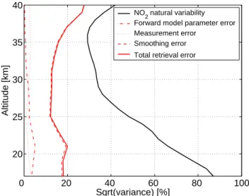
2 0 20 40 60 80 100 20 25 30 35 40 Sqrt(variance) [%] Altitude [km] NO2 natural variability Forward model parameter error Measurement error
Smoothing error Total retrieval error
Fig. 1. Example profiles of the smoothing, measurement, forward
model parameter, and total retrieval errors and profile of the NO2
natural variability. The retrieval errors are calculated for Harestua 25 May 2001 at sunset.
photochemical equilibrium assumptions are made. Updated kinetic and photochemical data are taken from the JPL 2000 compilation (Sander et al., 2000). Photolysis rates are com-puted off-line by using the radiative transfer module of the two-dimensional model SOCRATES (Huang et al., 1998).
The UVspec/DISORT RT model uses the discrete or-dinate method in a pseudo-spherical geometry approxima-tion in order to solve the RT equaapproxima-tion. All the calcula-tions are performed in multiple scattering mode and include Rayleigh scattering, Mie scattering (background conditions), and molecular absorptions. The ground albedo has been fixed to 25%, and the wavelengths used were 418 nm (Harestua) and 438 nm (Andøya). The variation of the concentration of the absorbing species along the light path has been taken into account since it has a large impact on the calculation of the slant column densities of rapidly photolysing species such as NO2 or BrO (Sinnhuber et al., 2002). Both RT and photo-chemical models have been validated through intercompari-son exercises (Hendrick et al., 2000, 2003).
4 Characterization of the retrieval 4.1 Error budget
The total error of the retrieved profile is the sum of three errors (Rodgers, 2000): the error due to the smoothing of the true profile or smoothing error, the error due to the mea-surement noise, and the error due to systematic errors in the forward model.
The smoothing error covariance matrix Ss can be calcu-lated using the following expression (Rodgers, 2000):
Ss=(A−I)Sx(A−I)T, (5)
−0.05 0 0.05 0.1 0.15 0.2 0 10 20 30 40 50 Altitude [km] 1 km 5 km 9 km 13 km 17 km 21 km 25 km 29 km 33 km 37 km 41 kmFig. 2. Typical example of ground-based NO2averaging kernels.
They are calculated for the sunset Harestua 25 May 2001 retrieval. Plain diamonds indicate the altitude at which each averaging kernel should peak in an ideal case.
where Sxis a realistic covariance matrix of the true NO2 pro-file, A is the averaging kernels matrix and I is the identity matrix. For the retrievals at Harestua, the variance of the true NO2profile placed on the diagonal of the Sxmatrix has been estimated from the HALOE NO2stratospheric profiles located in the 55◦N–65◦N latitude band over a period of five years (1998–2002). 1368 profiles were selected using these criteria, 437 at sunrise and 931 at sunset. They extend from end of February to mid-October, so that the seasonal variation of NO2 is largely taken into account. The use of the HALOE data for the present purpose has been limited to the 17–50 km altitude range (see Sect. 5.4 for a descrip-tion of the HALOE NO2observations). Due to the lack of large amounts of NO2observational data to make reasonable statistics below 17 km and above 50 km, the variance values calculated at 17 and 50 km from HALOE data have been ex-tended to all the levels below 17 km and above 50 km, re-spectively. Sxalso contains extra-diagonal terms in order to account for correlations between NO2values at different al-titude levels. These terms were added as Gaussian functions using the same expression and correlation length as for the Samatrix (see Eq. 2 in Sect. 3.1). Due to its latitude cover-age, HALOE reaches the latitude region of Andøya only for a limited number of days during the year. Therefore, the Sx matrix corresponding to this station cannot be constructed following a similar procedure as for Harestua (selection of
HALOE profiles in the 65◦N–75◦N). The most reasonable solution we found in this case has been to use, in a first ap-proximation, the Sxmatrix constructed for Harestua.
The contribution of the measurement noise to the total re-trieval error, also called the measurement error, is defined as (Rodgers, 2000): Sm=GSεGT (6) with G = ∂ _ x ∂y =(K TS−1 ε K + S −1 a ) −1KTS−1 ε , (7)
where Sε is the covariance matrix of the noise in the mea-surements, and G is the contribution functions matrix ex-pressing the sensitivity of the retrieved profile to changes in the measured NO2slant column abundances. As mentioned in Sect. 3.1, the Sε matrix was chosen diagonal with values corresponding to the statistical errors from the NO2DOAS fitting.
The forward model parameter error Sfis the retrieval error due to errors in the forward model parameters (e.g., errors on the rate constants in the photochemical model). Sfis given by the following expression (Rodgers, 2000):
Sf=G KbSbKTbG
T, (8)
where G is the contribution functions matrix (see Eq. 7), Kb is the sensitivity of the forward model to perturbations of for-ward model parameters b, and Sbis the covariance matrix of b. Sf cannot be determined easily due to the large number of forward model parameters. In the present study, we have used the Sf matrix derived by Preston et al. (1997) by cal-culating the sensitivity of the slant column measurements to large impact forward model (photochemical and/or RT mod-els) parameters like O3, HNO3, N2O5, aerosol, temperature profiles and ground albedo.
The profiles of the smoothing, measurement, and forward model parameter errors (square roots of the variances) cor-responding to the sunset Harestua 25 May 2001 retrieval as well as the NO2natural variability (square roots of the vari-ances of Sx)are shown in Fig. 1. The main contribution to the total retrieval error is clearly due to the smoothing error, both measurement and forward model errors being only minor er-ror sources. The total erer-ror is also significantly smaller than the NO2natural variability over the 17–37 km altitude range, which means that variations of the NO2profile smaller than the variations due to the natural variability can be detected from our GB UV-visible observations.
4.2 Information content analysis
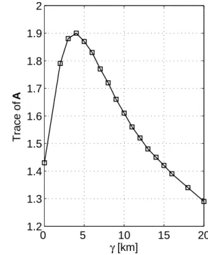
As mentioned in Sect. 3.1, the averaging kernel matrix A is the key parameter for the characterization of the retrievals. Typical NO2GB UV-visible averaging kernels are shown in Fig. 2. The averaging kernels between 13 km and 33 km are
0
5
10
15
20
1.2
1.3
1.4
1.5
1.6
1.7
1.8
1.9
2
γ [km]
Trace of
A
Fig. 3. Trace of the averaging kernels matrix A plotted as a function
of the HWHM (γ ). This curve has been calculated for the sunset Harestua 25 May 2001 retrieval.
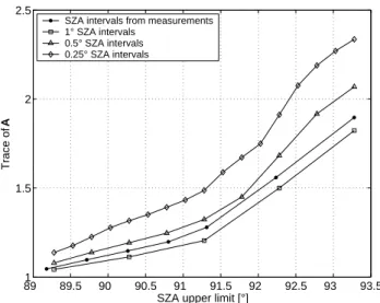
reasonably sharply peaked at their nominal altitude. From the examination of the averaging kernels for several dozens of sunsets and sunrises, it has been found that 13–37 km is the altitude range where the measurements give significant infor-mation about the vertical distribution of NO2. From Fig. 2, we also see that the vertical resolution is about 8 km at 13 km of altitude and reaches 20 km at an altitude of 33 km. Typical values for the trace of A are close to 2, so there are about 2 independent pieces of information in the measurements. The A matrix depends on the a priori covariance matrix Sa (see Eq. 3), and therefore on the correlation length between altitude levels used for the calculation of the extra-diagonal terms of Sa. The impact of this correlation length on the trace of A is large as it can be seen in Fig. 3 where the trace of A is plotted as a function of the γ parameter which is the half of the correlation length (see Eq. 2). The trace of A is maximun (1.9) for a correlation length of 8 km (γ =4 km) and the av-eraging kernels calculated with it are those shown in Fig. 2. Since such a feature has been obtained for a dozen of re-trievals performed at sunrise and sunset and corresponding to different seasonal conditions (early winter, spring, summer, and early fall), a correlation length of 8 km has been used in all our retrievals. The number of independent pieces of information also depends on the SZA sampling (SZA upper limit and intervals) of the measurements. To illustrate that, calculations of the trace of A have been performed using dif-ferent SZA upper limit values and three fixed SZA intervals (1◦, 0.5◦, and 0.25◦) in addition to the original SZA intervals
2 89 1 89.5 90 90.5 91 91.5 92 92.5 93 93.5 1.5 2 2.5 Trace of A
SZA upper limit [°]
SZA intervals from measurements 1° SZA intervals
0.5° SZA intervals 0.25° SZA intervals
Fig. 4. Impact of the SZA sampling (SZA upper limit and SZA
in-tervals) of the measurements on the number of independent pieces of information (trace of the averaging kernels matrix A). Synthetic measurements with fixed SZA intervals have been generated by us-ing a polynomial fit through the sunset Harestua 25 May 2001 mea-surements and interpolating on the desired SZA grid.
of the measurements. Synthetic measurements with fixed SZA intervals have been generated by using a polynomial fit through the sunset Harestua May 25, 2001 measurements and interpolating on the desired SZA grid. The results of the calculations appear in Fig. 4 where the trace of A is plotted as a function of the SZA upper limit for the four SZA intervals. Fig. 4 shows that the trace of A increases with a decrease of the SZA intervals: e.g., when the SZA upper limit is 93.28◦, the values of the trace of A for intervals of 1◦, 0.5◦, and 0.25◦ SZA are 1.82, 2.07, and 2.36, respectively, that means an in-crease of 30% from 1◦to 0.25◦SZA. As expected, the trace of A also increases with an increase of the SZA upper limit. 91.5◦ SZA seems to be a threshold value above which the increase of the trace of A with the SZA upper limit becomes faster (the slope below 91.5◦SZA is smaller than the slope above this SZA value). These results should be taken into ac-count when new DOAS instruments are developed in order to maximise the number of independent pieces of information contained in the measurements.
With the aim of quantifying the two independent pieces of information, an eigenvector expansion of the A matrix can be performed as for the characterization of ozone profiles re-trieved from solar infrared absorption spectra (Barret et al., 2002; see also Rodgers, 1990, 2000). From this eigenvector expansion of the A matrix and Eq. (3), the following expres-sion is derived:
_
z =3z + (I−3)za, (9)
where 3 is the diagonal matrix with the eigenvalues of A on its diagonal, and_z , z and za are the projections of the
state vectors _x , x, and xa on the right eigenvectors of A (_z =R−1_x ; z=R−1x, and z
a=R−1xa, where R is the matrix of the right eigenvectors of A). The 3 matrix being diagonal, Eq. (9) shows that we can decompose the state vector into patterns. Those for which the corresponding eigenvalues are close to 1 will be well reproduced by the measurement sys-tem, while those for which the corresponding eigenvalues are close to 0 will come mainly from the a priori state. Such an eigenvectors expansion has been applied to the typical NO2 GB UV-visible averaging kernels matrix shown in Fig. 2. The eigenvectors corresponding to the six largest eigenvalues are plotted in Fig. 5. The first eigenvalue is close to unity, im-plying a 100% contribution of the measurements in this pat-tern. This pattern also confirms that 13–37 km is the altitude range where significant information on the vertical distribu-tion of NO2 is present in the measurements. The next two patterns correspond to eigenvalues of 0.63 and 0.27, which means that both the measurements and the a priori contribute. For the last three patterns having eigenvalues close to 0, only the a priori state contributes.
5 Retrieval results – correlative comparisons
Our retrieval algorithm has been validated in the present study through comparison of the retrieved profiles with cor-relative data from the balloon-borne SAOZ and DOAS in-struments and the POAM III and HALOE satellite instru-ments. These balloon and satellite techniques have been cho-sen because they cover complementary altitude ranges (∼ 15–30 km for balloons and ∼ 20–45 km for satellites) and they all offer a good vertical resolution of about 1–2 km. Satellites also offer the advantage to operate year-round, al-lowing a larger number of coincident events with the GB ob-servations than the balloons.
The significant difference in vertical resolution between the GB and correlative profiles brings the concept of smooth-ing error into the comparison method. The NO2density pro-vided by a high-resolution correlative instrument contains in-formation confined to only a few km around the retrieval alti-tude. For the same retrieval altitude, the information coming from a GB measurement spreads over a much larger altitude range. This drastic difference in perception of the true NO2 profile affects direct comparisons with large smoothing er-rors. One way to reduce these errors is to degrade the high-resolution of the satellite and balloon profiles to the lower resolution of GB profiles using the following adaptation of Eq. (3) (Connor et al., 1994):
xs=xa+A(xc−xa), (10)
where A is the GB UV-visible averaging kernels matrix, xa is the a priori profile used in the retrieval, xcis the correlative profile, and xsis the smoothed or convolved profile, which is what the retrieval should produce assuming that xcis the true profile and that the only source of error is the smoothing error
−0.5 0 0.5 0 10 20 30 40 50 Altitude [km] λ = 0.99622 −0.5 0 0.5 0 10 20 30 40 50 λ = 0.63026 −0.5 0 0.5 0 10 20 30 40 50 λ = 0.26704 −0.5 0 0.5 0 10 20 30 40 50 Altitude [km] λ = 0.00214 −0.5 0 0.5 0 10 20 30 40 50 λ = 0.00042 −0.5 0 0.5 0 10 20 30 40 50 λ = 0.00005
Fig. 5. Typical leading eigenvectors of the A matrix and their corresponding eigenvalues. They are calculated for the sunset Harestua 25
May 2001 retrieval.
(see Eq. 3). The correlative profiles cover a limited altitude range (e.g., ∼ 13–29 km for the SAOZ balloon) but according to the smoothing method used (see Eq. 10), they have to be extended over the same altitude grid as the averaging kernels. In the present study, they have been completed below and above the covered altitude range by the a priori profile scaled by the ratios between the correlative and a priori profiles at the lower and upper altitude limits of the correlative profile, respectively; e.g. a SAOZ balloon profile is completed be-low 13 km by the a priori profile scaled by the ratio between the SAOZ balloon and a priori profiles at 13 km, and above 29 km by the a priori profile scaled by the ratio of the SAOZ balloon and a priori profiles at 29 km. This scaling avoids the presence of large discontinuities at the lower and upper limits of the original altitude range of the correlative profile. Each retrieval has also been quality-checked by comparing the absolute slant column densities (SCDs) calculated using the retrieved profile and the measured ones. The SCDs cal-culated with the retrieved profile fit generally very well with the measurements as can be seen in Fig. 6. This plot also illustrates the difference between the SCDs calculated using the a priori and retrieved profiles.
5.1 SAOZ balloon comparisons
The SAOZ balloon gondola is a UV-visible spectrometer able to provide vertical profiles of O3, NO2, OClO, BrO and H2O
75 80 85 90 95 0 2 4 6 8 10 12 14 16 18 SZA [°] NO 2 SCD [x10 16 molec/cm 2 ] measurements calc. with a priori profile calc. with retrieved profile
Fig. 6. Comparison between measurements and SCDs calculated
using the a priori and retrieved profiles for the sunset Harestua 25 May 2001 retrieval. The error bars on the measurements are contained within the symbols (typical error values amount to 5×10¹⁴molecules/cm2and correspond to one standard deviation of the statistical error from the DOAS fitting).
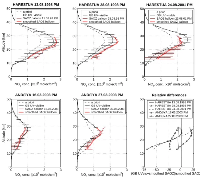
2 0 1 2 3 0 10 20 30 40 50 NO 2 conc. [x10 9 molec/cm3] Altitude [km] HARESTUA 13.08.1998 PM a priori GB UV−visible SAOZ balloon 11.08.98 PM smoothed SAOZ balloon
0 1 2 3 0 10 20 30 40 50 NO 2 conc. [x10 9 molec/cm3] HARESTUA 28.08.1998 PM a priori GB UV−visible SAOZ balloon 28.08.98 PM smoothed SAOZ balloon
0 1 2 3 0 10 20 30 40 50 AND∅YA 27.03.2003 PM NO 2 conc. [x10 9 molec/cm3] a priori GB UV−visible SAOZ balloon 30.03.2003 smoothed SAOZ balloon
0 1 2 3 0 10 20 30 40 50 AND∅YA 16.03.2003 PM NO 2 conc. [x10 9 molec/cm3] Altitude [km] a priori GB UV−visible SAOZ balloon 16.03.2003 smoothed SAOZ balloon
0 1 2 3 0 10 20 30 40 50 NO 2 conc. [x10 9 molec/cm3] HARESTUA 24.08.2001 PM a priori GB UV−visible SAOZ balloon 23.08.01 PM smoothed SAOZ balloon
−750 −50 −25 0 25 10 20 30 40 50
(GB UVvis−smoothed SAOZ)/smoothed SAOZ [%]
Relative differences HARESTUA 13.08.1998 PM HARESTUA 28.08.1998 PM HARESTUA 24.08.2001 PM AND∅YA 16.03.2003 PM AND∅YA 27.03.2003 PM
Fig. 7. Comparison between ground-based UV-visible profiles at Harestua (sunset, summer conditions) and Andøya (sunset, late winter-early
spring conditions) and SAOZ balloon profiles. In the 5 cases, SAOZ balloons were launched from Kiruna. For direct comparison, SAOZ balloon profiles have been smoothed by convolving them with the ground-based UV-visible averaging kernels. The relative differences appear in the right lower plot.
during the ascent at sunset or descent at sunrise of the bal-loon and from float at 30 km (solar occultation). The balbal-loon version of the SAOZ instrument is very similar to the one used for GB measurements (Pommereau and Goutail, 1988). NO2is measured in the spectral region from 410 to 530 nm using the cross sections measured at 220 K by Vandaele et al. (1998). All the flights used for the GB-SAOZ balloon comparisons originated in Kiruna (68◦N, 21◦E) in Sweden and occurred at sunset. Since the SAOZ balloon NO2data have not been corrected for photochemical variations along the line of sight, only the ascent data are taken into account for the comparisons. These are provided with a vertical res-olution of 1 km. Five coincident events were found between the GB and balloon observations: three in summer condi-tions (Harestua GB data) and two in early spring condicondi-tions (Andøya GB data). GB UV-visible data are not always
avail-able for the days where SAOZ balloon flights occur. There-fore, several days can separate GB and balloon-borne obser-vations. Due to the rather large latitude difference (8◦) be-tween Harestua and Kiruna, comparisons are only relevant in summer conditions where stable air masses are present most of the time above this latitude region (60◦N–70◦N). This is in contrast with winter and early spring conditions where large dynamical effects occur, especially above Harestua that is often located close to the edge of the wintertime polar vor-tex. Most of the time air masses with different histories are therefore probed from both stations making the profile com-parisons irrelevant.
The results of the comparisons with SAOZ balloon pro-files are shown in Fig. 7. The agreement obtained between GB UV-visible and smoothed SAOZ balloon profiles is good for the Harestua 13 and 28 August and Andøya 16 March
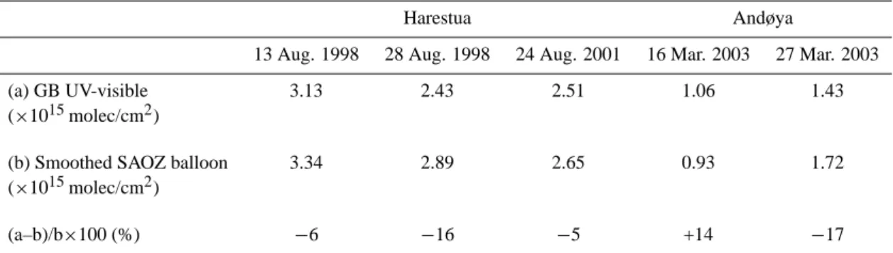
Table 1. 13–29 km NO2partial columns values calculated from coincident ground-based UV-visible and smoothed SAOZ balloon profiles
at Harestua and Andøya at sunset. In the 5 cases, the SAOZ balloons were launched from Kiruna. The relative differences in % appear in the third row.
Harestua Andøya
13 Aug. 1998 28 Aug. 1998 24 Aug. 2001 16 Mar. 2003 27 Mar. 2003 (a) GB UV-visible 3.13 2.43 2.51 1.06 1.43 (×1015molec/cm2)
(b) Smoothed SAOZ balloon 3.34 2.89 2.65 0.93 1.72 (×1015molec/cm2)
(a–b)/b×100 (%) −6 −16 −5 +14 −17
Table 2. 13–37 km NO2partial columns values calculated from coincident ground-based UV-visible and smoothed DOAS balloon profiles
at Harestua at sunset. In both cases, the DOAS balloons were launched from Kiruna. The relative differences in % appear in the third row. 19 Aug. 1998 19 Aug. 2001
(a) GB UV-visible (×1015molec/cm2) 4.01 4.24 (b) smoothed DOAS balloon (×1015molec/cm2) 4.10 3.41
(a–b)/b×100 (%) −2 +24
cases, both profiles differing over the entire 13–29 km alti-tude range by less than 7%, 25%, and 21%, respectively. For both other coincident days, the relative difference is smaller than 25% above 20 km but larger discrepancies are observed below this altitude level (relative difference up to 70%). For the Andøya 27 March case, dynamical effects could be ar-gued to explain the observed discrepancies since it is the end of the NH vortex season and three days elapsed between the GB and balloon-borne observations. However, a check of the potential vorticity at 475 K has shown that both balloon and GB measurements were performed outside the polar vortex.
The 13–29 km NO2 partial column values calculated by integrating the GB UV-visible and smoothed SAOZ balloon profiles are presented in Table 1. The comparison gives good agreement since partial column values differ by less than 17% for the 5 coincident events.
5.2 DOAS balloon comparisons
The DOAS balloon instrument is extensively described in Ferlemann et al. (2000). It consists of two thermostated (273 K) grating spectrometers in which the UV (316– 418 nm) and visible (399.9–653 nm) parts of the sunlight are analyzed separately. Light detection is performed with two cooled photodiode array detectors (1024 diodes, 263 K). As it is designed, the instrument can provide atmospheric col-umn abundances or profiles of O3, NO2, NO3, IO, OIO,
OClO, BrO, O4, CH2O, and H2O. Among the ten flights of the DOAS instrument successfully conducted until now, two – originating from Kiruna – are appropriate for comparison with the Harestua GB UV-visible data. These are 19 August 1998 and 21 August 2001 at sunset. For the same reason as for the SAOZ balloons, only ascent data are used here. Concerning the second flight, the only day around 21 August 2001 where GB UV-visible data are available at Harestua is 19 August 2001.
The results of the profiles comparison for both coincident days are shown in Fig. 8. A good agreement is observed be-tween the GB profile inversion and the DOAS balloon for the 19 August 1998 case where the relative difference be-tween both profiles is smaller than 4% over the whole alti-tude range. Concerning the 19 August 2001 comparison, the GB UV-visible profile is clearly above the smoothed DOAS balloon one in the 15–39 km altitude range, with a maximum overestimation of 30% near 27 km.
The 13–37 km NO2partial column values calculated from the GB UV-visible and smoothed DOAS balloon profiles are presented in Table 2. A reasonably good agreement is ob-served since GB profile inversion and balloon differ by −2% and +24% in the 19 August 1998 and 2001 cases, respec-tively.
2 0 10 20 30 0 10 20 30 40 50
(GB UVvis−smoothed DOAS)/smoothed DOAS [%]
Relative differences HARESTUA 19.08.1998 PM HARESTUA 19.08.2001 PM 0 1 2 3 0 10 20 30 40 50 NO 2 conc. [x10 9 molec/cm3] HARESTUA 19.08.2001 PM a priori GB UV−visible DOAS balloon 21.08.01 PM smoothed DOAS balloon
0 1 2 3 0 10 20 30 40 50 NO 2 conc. [x10 9 molec/cm3] Altitude [km] HARESTUA 19.08.1998 PM a priori GB UV−visible DOAS balloon 19.08.98 PM smoothed DOAS balloon
Fig. 8. Comparison between ground-based UV-visible profiles at Harestua and DOAS balloon profiles for two sunsets in summer conditions.
DOAS balloons were launched from Kiruna. For direct comparison, DOAS balloon profiles have been smoothed by convolving them with the ground-based UV-visible averaging kernels. The relative differences appear in the right plot.
5.3 POAM III comparisons
POAM III is a nine-channel (0.354–1.018 µm) solar oc-cultation instrument launched onboard the Satellite Pour l’Observation de la Terre (SPOT) 4 in March 1998 (Randall et al., 2002). It has been designed to measure stratospheric profiles of O3, NO2 and water vapor densities, as well as aerosol extinction and temperature. NO2 densities are re-trieved from 20 to 45 km through differential measurements at 439.6 nm (NO2-“on” channel) and 442.2 nm (NO2-“off” channel). The vertical resolution is about 2 km at altitudes below 40 km and decreases to more than 7 km at an altitude of 45 km. The POAM III retrievals do not include a correc-tion for the diurnal variacorrec-tion of NO2along a solar occulta-tion measurement line of sight. The criterion used for spatial coincidence is location of the POAM III profiles at tangent point within 5◦latitude and 5◦longitude of Harestua. Con-cerning the temporal coincidence, days of POAM III and GB observations are the same. 76 coincident events were found during the period from mid-June 1998 to mid-September 2000, 39 and 37 sunsets in spring and summer conditions, respectively.
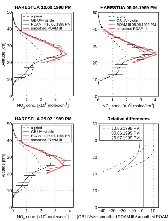
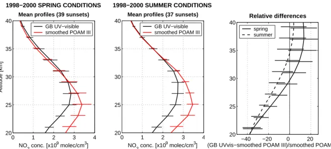
Examples of profile comparisons are shown in Fig. 9. A good agreement is obtained for 10 June 1998 and 5 June 1999 coincident events: the relative difference is smaller than 25% in the whole altitude range. For both cases, the largest rel-ative difference values are observed below 25 km with GB UV-visible inversion smaller than POAM III. This underesti-mation of the POAM III data by the GB UV-visible retrievals at low altitude levels is larger in the third case (25 July 1999) with difference values up to 40%. This behaviour is sys-tematic since it clearly appears when profiles are averaged, as illustrated in Fig. 10. Averages for spring and summer
conditions have been plotted separately because of the dif-ference in the polar vortex conditions between both seasons at Harestua (possible presence and absence of the polar vor-tex in spring and summer, respectively). Figure 10 shows that the magnitude of the underestimation is similar in both spring and summer. Its possible origin is discussed later in Sect. 5.4 since it is also observed in the comparisons with HALOE profiles.
The 20–37 km NO2 partial columns are compared in Fig. 11. This altitude range has been chosen because it is the common range where GB UV-visible retrieval and POAM III give reliable information on the vertical distribution of the NO2 concentration. Except for two coincident days in 2000, the GB UV-visible columns underestimate the POAM III data by maximum 26%. In their validation study of POAM III NO2 measurements, Randall et al. (2002) have compared the 20–45 km POAM III NO2partial columns to total columns measured at Kiruna using a GB UV-visible spectrometer. They found that POAM III underestimates the GB total columns, mainly because an expected low bias is present in the POAM III data since they do not include the tropospheric, lower stratospheric, and upper stratospheric NO2seen by the GB instruments. Such an underestimation (up to 30%) by POAM III is also observed when the POAM III 20–37 km NO2partial columns are compared to the to-tal columns calculated from our retrieved profiles, meaning that results consistent with those of Randall et al. (2002) can be obtained when we use their comparison method. These results are not shown here because we found that compar-ing GB total and POAM III partial columns is not the most appropriate method of comparison.
Fig. 11 also shows that the relative difference between the GB UV-visible and smoothed POAM III 20–37 km NO2
0 1 2 3 4 0 10 20 30 40 50 NO 2 conc. [x10 9 molec/cm3] Altitude [km] HARESTUA 10.06.1998 PM a priori GB UV−visible POAM III 10.06.1998 PM smoothed POAM III
0 1 2 3 4 0 10 20 30 40 50 NO 2 conc. [x10 9 molec/cm3] HARESTUA 05.06.1999 PM a priori GB UV−visible POAM III 05.06.1999 PM smoothed POAM III
−40 −30 −20 −10 0 10 0 10 20 30 40 50
(GB UVvis−smoothedPOAMIII)/smoothedPOAMIII [%]
Relative differences 10.06.1998 PM 05.06.1999 PM 25.07.1999 PM 0 1 2 3 4 0 10 20 30 40 50 NO 2 conc. [x10 9 molec/cm3] Altitude [km] HARESTUA 25.07.1999 PM a priori GB UV−visible POAM III 25.07.1999 PM smoothed POAM III
Fig. 9. Examples of comparison between ground-based UV-visible and POAM III profiles at Harestua (sunset conditions). For direct
comparison, POAM III profiles have been smoothed by convolving them with the ground-based UV-visible averaging kernels. The relative differences appear in the right lower plot.
partial columns varies from year to year, especially between spring 1999 and spring 2000 where mean relative difference values of −18% and −8% are observed, respectively. 5.4 HALOE comparisons
HALOE was launched on board the Upper Atmosphere Re-search Satellite (UARS) in September 1991 (Gordley et al., 1996). As for POAM III, the satellite instrument probes the atmosphere in solar occultation. Vertical profiles of
tempera-ture, O3, HCl, HF, CH4, NO, NO2, and aerosol extinction are inferred from two infrared channels centered at 5.26 µm and 6.25 µm. The HALOE NO2measurements extend from the lower stratosphere (∼10 km) to 50 km of altitude. However, large error bars are sometimes observed below 25 km, the er-ror bars becoming larger as the altitude decreases. Due to this reduction of reliability in the lower stratosphere, only HALOE data corresponding to altitude levels higher than 20 km have been used for the comparison. In this altitude range (20–50 km), the vertical resolution of the HALOE
2 0 1 2 3 4 20 25 30 35 40
Mean profiles (39 sunsets) 1998−2000 SPRING CONDITIONS NO 2 conc. [x10 9 molec/cm3] Altitude [km] GB UV−visible smoothed POAM III
0 1 2 3 4 20 25 30 35 40 1998−2000 SUMMER CONDITIONS Mean profiles (37 sunsets)
NO2 conc. [x109 molec/cm3]
GB UV−visible smoothed POAM III
−40 −20 0 20 20 25 30 35 40
(GB UVvis−smoothed POAM III)/smoothed POAM III [%]
Relative differences
spring summer
Fig. 10. Comparison of averaged ground-based UV-visible and smoothed POAM III profiles for sunset spring (left plot) and sunset summer
(middle plot) conditions at Harestua for the period from mid-June 1998 to mid-September 2000. The relative differences appear in the right plot. The error bars represent the standard deviations of the GB, POAM III, and relative difference profiles. They are offset high by 0.2 km on the smoothed POAM III and summer relative difference profiles for clarity.
Jan Apr Jul Oct Jan Apr Jul Oct Jan Apr Jul Oct Jan 0 1 2 3 4 5 NO 2 partial column [x10 15 molec/cm 2] GB UV−visible smoothed POAM III
Jan Apr Jul Oct Jan Apr Jul Oct Jan Apr Jul Oct Jan −30 −20 −10 0 Relative difference [%] 1998 1999 2000
(GB UVvis−smoothed POAM III)/smoothed POAM III
Fig. 11. Comparison of the sunset 20–37 km NO2 partial
columns calculated from the coincident ground-based UV-visible and smoothed POAM III profiles at Harestua for the period 1998– 2000. The relative differences appear in the lower plot.
observations of NO2is 2 km. In contrast to POAM III, the HALOE processing algorithm includes a basic correction for the line of sight gradients of NO2 concentration across the limb due to the marked diurnal variation of this species. As for POAM III comparisons, the criterion used for spatial co-incidence is location of the HALOE profiles at tangent point
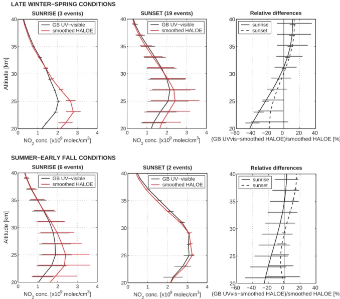
within 5◦latitude and 5◦longitude of Harestua. Concerning the temporal coincidence, days of HALOE and GB observa-tions are the same. Using these criteria, 22 coincident events (3 at sunrise and 19 at sunset) were found for late winter-spring conditions and 8 (6 at sunrise and 2 at sunset) for the summer-early fall period.
Figure 12 shows the comparison in the 20–40 km al-titude range between the GB UV-visible and smoothed HALOE NO2 profiles averaged for late winter-early spring and summer-early fall conditions, sunrise and sunset being treated separately. Comparison results above 40 km are not shown since there is no information any more on the verti-cal distribution of NO2 above ∼37 km in the GB measure-ments and it is therefore essentially a comparison with the a priori profile. Both GB profile inversion and HALOE agree well above ∼28 km. Below this altitude, a systematic un-derestimation of the HALOE data by the GB profile inver-sion occurs as in the POAM III comparisons, although the observed differences are here within the variability of both profiles (except in late winter-spring at sunrise but the statis-tics significance is poor in these conditions). The compar-ison of Fig. 10 and 12 also shows that the agreement with HALOE at sunset is significantly better than with POAM III for both spring and summer conditions (relatives differences below 25 km smaller than 20% instead of being comprised between 20% and 40% for POAM III). A problem in the GB profile retrievals cannot be the main cause of the system-atic underestimation of the satellite data by the GB retrievals since a good agreement has been observed with the SAOZ and DOAS balloons in the 20–25 km range, balloon data being the most suitable correlative observations available
0 1 2 3 4 20 25 30 35 40 SUNRISE (3 events)
LATE WINTER−SPRING CONDITIONS
NO 2 conc. [x10 9 molec/cm3] Altitude [km] GB UV−visible smoothed HALOE 0 1 2 3 4 20 25 30 35 40 SUNSET (19 events) NO 2 conc. [x10 9 molec/cm3] GB UV−visible smoothed HALOE 0 1 2 3 4 20 25 30 35 40 SUNSET (2 events) NO 2 conc. [x10 9 molec/cm3] GB UV−visible smoothed HALOE −60 −40 −20 0 20 40 20 25 30 35 40
(GB UVvis−smoothed HALOE)/smoothed HALOE [%]
Relative differences sunrise sunset −60 −40 −20 0 20 40 20 25 30 35 40
(GB UVvis−smoothed HALOE)/smoothed HALOE [%]
Relative differences sunrise sunset 0 1 2 3 4 20 25 30 35 40 SUNRISE (6 events)
SUMMER−EARLY FALL CONDITIONS
NO 2 conc. [x10 9 molec/cm3] Altitude [km] GB UV−visible smoothed HALOE
Fig. 12. Comparison of coincident ground-based UV-visible and smoothed HALOE profiles separately averaged for sunrise and sunset for
late winter-spring (upper plots) and summer-early fall (lower plots) conditions at Harestua. The coincident events cover the period from mid-June 1998 to mid-September 2001. The relative differences appear in the right plots. The error bars represent the standard deviations of the GB, HALOE, and relative difference profiles. They are offset high by 0.2 km on the smoothed HALOE and sunset relative difference profiles for clarity.
to validate our retrievals in this altitude range. Therefore, this feature would be more likely due to a limitation of the HALOE and POAM III instruments for measuring NO2at these low altitude levels. The possible error sources on the HALOE and POAM III data are described in detail in Gord-ley et al. (1996) and Randall et al. (2002). A source of sys-tematic error is the strong variations of NO2 along a solar occultation measurement line of sight. Neglecting a correc-tion for the line of sight variacorrec-tions can result in a systematic overestimation in NO2below 25 km. According to Randall et al. (2002) and Newchurch et al. (1996), this overestimation is ∼20% at 20 km whereas Roscoe and Pyle (1987) estimate it to maximum 1% for the conditions of the present com-parisons. The uncertainty on the diurnal effect correction is
therefore very large, mainly because this correction strongly depends on the photochemical model (including the initial-ization settings) used for calculating it. Nevertheless, the ab-sence of such a correction in the POAM III retrievals could at least partly explain the large discrepancies systematically observed between the GB profile retrievals and POAM III below 25 km since this explanation is consistent with the sig-nificantly better agreement observed with HALOE – which includes a correction for the diurnal effect – than with POAM III in sunset spring and summer conditions. The comparison of the relative differences in these conditions (below 20% for HALOE and comprised between 20% and 40% for POAM III) suggests that the magnitude of the diurnal effect correc-tion could reach at least 10%. This effect could also play
2
Mar0 Apr May Jun Jul Aug Sep Oct
1 2 3 4 5 NO 2 partial column [x10 15 molec/cm 2] GB UV−visible @ sunrise GB UV−visible @ sunset smoothed HALOE @ sunrise smoothed HALOE @ sunset
Mar Apr May Jun Jul Aug Sep Oct
−40 −20 0 20 40 Relative difference [%]
(GB UVvis−smoothed HALOE)/smoothed HALOE @ sunrise (GB UVvis−smoothed HALOE)/smoothed HALOE @ sunset
Fig. 13. Comparison of the 20–37 km NO2partial columns
calcu-lated from the coincident ground-based UV-visible and smoothed HALOE profiles at Harestua. Due to the small number of coincident events, the sunrise and sunset partial columns for the 1998–2001 pe-riod have been gathered in the same plot. The relative differences appear in the lower plot.
a significant role in the difference observed between sun-rise and sunset in the agreement between GB retrievals and HALOE data (larger discrepancies at sunrise than at sunset) since the uncertainty on it can be 2 to 3 times larger at sun-rise than at sunset (Gordley et al., 1996). More investiga-tions - which are beyond the scope of the present study – are required to go one step further in the determination of the exact impact of this error source as well as others (e.g. the errors due to interfering absorbers and uncertainties on spec-tral parameters) on the agreement between GB retrievals and satellite instruments.
The 20–37 km GB UV-visible and HALOE NO2 partial columns are compared in Fig. 13. As for the comparison with POAM III, the 20–37 km altitude range has been chosen be-cause it is the common range where data from GB UV-visible retrieval and HALOE are reliable. Due to the small number of coincident events, the sunrise and sunset partial columns for the 1998–2001 period have been gathered in the same plot and not plotted separately for sunrise and sunset and for each year as in the comparison with POAM III. Except for 7 coin-cident events (1 at sunrise and 6 at sunset) over a total number of 30, the GB retrievals underestimate the HALOE data. At sunset, the absolute value of the relative difference between the GB and smoothed HALOE partial columns is most of the time (18 coincident events over a total number of 21) smaller than 20%, a maximum value of 28% being reached in March. During this late winter-early spring period where large dynamical effects occur above Harestua and the NO2 concentration is low, a large scatter is also observed in the
relative differences between the GB UV-visible and HALOE data. At sunrise, the absolute value of the relative difference is comprised between 20% and 28% and is below 20% for 5 and 4 coincident events, respectively. In the HALOE NO2 validation study of Gordley et al. (1996), the HALOE col-umn amounts above the 80 mb pressure level (∼17 km) have been compared to the total column amounts measured by a GB spectrometer at Fritz Peak, Colorado (40◦N, 106◦W). Days with significant tropospheric contribution have been excluded from the comparison. The HALOE observations were found to be lower than the GB ones by 10–30%, mainly due to the fact that the HALOE column amounts above 80 mb do not include the lower stratospheric NO2seen by the GB instrument. We have observed similar differences (15– 40%) when the HALOE 20–37 km partial columns are com-pared to the NO2total columns calculated from our retrieved GB UV-visible profiles. Using the same method of com-paring columns, results consistent with those of Gordley et al. (1996) can therefore be obtained. As for POAM III, these results are not shown here because the comparison method of Gordley et al. (1996) is not the most appropriate due the difference in the altitude ranges where the GB and HALOE columns are calculated.
6 Conclusions
NO2 stratospheric profiles have been retrieved from GB zenith-sky UV-visible observations using the OEM. The re-trieval algorithm has been applied to observational data sets from the NDSC stations of Harestua and Andøya in Nor-way. The characterization of the retrievals has been per-formed as in the study of Barret et al. (2002) on the retrieval of ozone profiles from solar infrared absorption spectra. We have shown that about 2 independent pieces of information are contained in the measurements. Both components have been quantified from an eigenvector expansion of the aver-aging kernels matrix A. We have also determined the impact on the number of independent pieces of information of the SZA sampling of the measurements and the extra-diagonal terms of the a priori covariance matrix. Concerning the er-ror analysis, the profiles of the smoothing, measurement, and forward model parameter errors have been compared to the NO2natural variability. The smoothing error clearly appears to be the main source of error. The total retrieval error is also well below the NO2natural variability, pointing out that vari-ations of the NO2profile smaller than the natural variability can be detected from our GB UV-visible observations.
Retrieved NO2stratospheric profiles and partial columns have been validated through comparisons with correlative balloon and satellite observations. Although the number of coincident events was too small to constitute a statistically significant comparison, a good agreement was generally found with SAOZ and DOAS balloons, especially in the 20–30 km altitude range. Concerning the partial columns
between 13 and 29 km and 13 and 37 km for SAOZ and DOAS balloons, respectively, the relative difference reached a maximum value of 24%. The correlative comparisons with the POAM III and HALOE satellite data showed a poorer agreement with our retrievals than those with the balloon data. When mean profiles were compared, the GB UV-visible retrievals systematically underestimated the satellite instruments below 25–27 km where the relative differences were generally comprised between 20% and 40%. Since (1) this feature was observed for POAM III and HALOE data, and (2) a good agreement was found in the 20–30 km range with balloon measurements, it could be more likely due to a common limitation of both satellite solar occultation in-struments at these low altitude levels. The impact on this systematic underestimation of a correction for the NO2 pho-tochemical variation along a solar occultation measurement line of sight has been discussed. The comparison of par-tial columns between 20 and 37 km showed a better agree-ment with relative difference values smaller than 26% and 28% for POAM III and HALOE, respectively. We have also verified that using the same way of comparing columns, i.e. comparing the POAM III and HALOE partial columns to the GB total columns, results consistent with the POAM III and HALOE validation studies of Randall et al. (2002) and Gord-ley et al. (1996) can be obtained.
The results of the present work – especially those con-cerning the characterization of the retrievals and the exten-sive comparison exercise with correlative data – strengthen our confidence in the reliability and the robustness of the re-trieval of the vertical distribution of stratospheric trace gas species from GB zenith-sky UV-visible observations. This technique offers new perspectives in the use of GB UV-visible networks such as the NDSC for the purpose of valida-tion of satellite and balloon experiments as well as modelling data. Moreover, its application to combined observations in zenith, direct-sun, and off-axis (pointing towards the hori-zon) geometries – made possible due to recent instrumen-tal developments in DOAS spectroscopy (H¨onninger et al., 2004; Heckel et al., 2004) – will allow to retrieve informa-tion on the vertical distribuinforma-tion in both the stratosphere and troposphere, which is particularly important for species like BrO and NO2.
Acknowledgements. This research was financially supported by
the Belgian Federal Science Policy Office (contracts ESAC II EV/35/3A and MO/35/006 & 012) and the European Commission (contract QUILT, EVK2-2000-00545). M. P. Chipperfield (Uni-versity of Leeds) is greatly acknowledged for providing us with the SLIMCAT data. We wish also to thank the POAM III and HALOE Science and Processing Teams. Finally, we are thankful to C. Fayt (IASB-BIRA) for her contribution to the observations at the Harestua and Andøya stations, and to L. Denis, H. K. Roscoe (BAS), and R. Schofield (NIWA) for fruitful discussions.
Edited by: J. Burrows
References
Barret, B., De Mazi`ere, M., and Demoulin, P.: Retrieval and characterisation of ozone profiles from solar infrared spec-tra at the Jungfraujoch, J. Geophys. Res., 107 (D24), 4788, doi:10.1029/2001JD001298, 2002.
Brewer, A. W., McElroy, C. T., and Kerr, J. B.: Nitrogen dioxide concentration in the atmosphere, Nature, 246, 129–133, 1973. Chipperfield, M. P.: Multiannual simulations with a
three-dimensional chemical transport model, J. Geophys. Res., 104 (D1), 1781–1805, 1999.
Connor, B. J., Siskind, D. E., Tsou, J. J., Parrish, A., and Remsberg, E. E.: Ground-based microwave observations of ozone in the upper stratosphere and mesosphere, J. Geophys. Res., 99 (D8), 16 757–16 770, 1994.
Errera, Q. and Fonteyn, D.: Four-dimensional variational chemi-cal assimilation of CRISTA stratospheric measurements, J. Geo-phys. Res., 106 (D11), 12 253–12 265, 2001.
Ferlemann, F., Bauer, N., Fitzenberger, R., Harder, H., Osterkamp, H., Perner, D., Platt, U., Schneider, M., Vradelis, P., and Pfeil-sticker, K.: Differential Optical Absorption Spectroscopy Instru-ment for stratospheric balloon-borne trace gas studies, Applied Optics, 39, 2377–2386, 2000.
Gordley, L. L., Russel III, J. M., Mickley, L. J., et al.: Validation of nitric oxide and nitrogen dioxide measurements made by the Halogen Occultation Experiment for UARS platform, J. Geo-phys. Res., 101 (D6), 10 241–10 266, 1996.
Hendrick, F., Mueller, R., Sinnhuber, B.-M., et al.: Simulation of BrO Diurnal Variation and BrO Slant Columns: Intercompari-son Exercise Between Three Model Packages, Proceedings of the 5th European Workshop on Stratospheric Ozone, Saint Jean de Luz, France, 27 Sept.–1 Oct. 1999, Air Pollution Research Report n◦73, European Commission – DG XII, Brussels, 2000. Hendrick, F., Van Roozendael, M., Kylling, A., Wittrock, F.,
von Friedeburg, C., Sanghavi, S., Petritoli, A., Denis, L., and Schofield, R.: Report on the workshop on radiative transfer mod-eling held at IASB-BIRA, Brussels, Belgium, on 3–4 October 2002, WP 2500 of the QUILT project (European commission, EVK2-CT2000-00059), http://nadir.nilu.no/quilt, 2003. Heckel, A., Richter, A., Tarsu, T., Wittrock, F., Hak, C., Pundt, I.,
Junkermann, W., and Burrows, J. P.: MAX-DOAS measurements of formaldehyde in the Po-Valley, Atmos. Chem. Phys. Discuss., 4, 1151–1180, 2004,
SRef-ID: 1680-7375/acpd/2004-4-1151.
Heskes, H. J. and Boersma, K. F.: Averaging kernels for DOAS total-column satellite retrievals, Atmos. Chem. Phys., 3, 1285– 1291, 2003,
SRef-ID: 1680-7324/acp/2003-3-1285.
H¨onninger, G., von Friedeburg, C., and Platt, U.: Multi axis dif-ferential optical absorption spectroscopy (MAX-DOAS), Atmos. Chem. Phys., 4, 231–254, 2004,
SRef-ID: 1680-7324/acp/2004-4-231.
Huang, T., Walters, S., Brasseur, G., et al.: Description of SOCRATES – A Chemical Dynamical Radiative Two– Dimensional Model, NCAR technical note no. TN–440+EDD, National Center for Atmospheric Research, Boulder, Colorado, 1998.
Kylling, A. and Mayer, B.: LibRadTran: A package for UV and visible radiative transfer calculations in the Earth’s atmosphere, http://www.libradtran.org, 2003.
2
Lee, A. M., Roscoe, H. K., Oldham, D. J., Squires, J. A. C., Sarkissian, A., and Pommereau, J.-P.: Improvements to the ac-curacy of zenith-sky measurements of NO2by visible spectrom-eters, J. Quant. Spectr. Rad. Transfer, 52, 649–657, 1994. McKenzie, R., Johnston, P. V., McElroy, C. T., Kerr, J. B., and
Solomon, S.: Altitude distributions of stratospheric constituents from ground-based measurements at twilight, J. Geophys. Res., 96 (D8), 15 499–15 511, 1991.
Newchurch, M. J., Allen, M., Gunson, M. R., et al.: Stratospheric NO and NO2abundances from ATMOS solar-occultation mea-surements, Geophys. Res. Lett., 23, 2373–2376, 1996.
Noxon, J. F.: Nitrogen dioxide in the stratosphere and troposphere measured by ground-based absorption spectroscopy, Science, 189, 547–549, 1975.
Platt, U.: Differential Optical Absorption Spectroscopy (DOAS), in: Air Monitoring By Spectroscopic Techniques, edited by: Sigrist, M. W., John Wiley and Sons, Inc., New York, 1994. Pommereau, J. P. and Goutail, F.: O3 and NO2 ground-based
measurements by visible spectrometry during Arctic winter and spring 1988, Geophys. Res. Lett., 15, 891–894, 1988.
Preston, K. E., Jones, R. L., and Roscoe, H. K.: Retrieval of NO2
vertical profiles from ground-based UV-visible measurements: Method and validation, J. Geophys. Res., 102 (D15), 19 089– 19 097, 1997.
Randall, C. E., Lumpe, J. D., Bevilacqua, R. M., et al.: Validation of POAM III NO2measurements, J. Geophys. Res., 107 (D20), 4432, doi:10.1029/2001JD001520, 2002.
Rodgers, C. D.: Retrieval of atmospheric temperature and composi-tion from remote measurements of thermal radiacomposi-tion, Rev. Geo-phys. Space Phys., 14 (4), 609–624, 1976.
Rodgers, C. D.: Characterisation and error analysis of profiles re-trieved from remote sounding measurements, J. Geophys. Res., 95 (D5), 5587–5595, 1990.
Rodgers, C. D.: Inverse Methods for Atmospheric Sounding, The-ory and Practice, World Scientific Publishing, Singapore – New-Jersey – London – Hong Kong, 2000.
Roscoe, H. K. and Pyle, J. A.: Measurements of solar occultation: the error in a naive retrieval if the constituent’s concentration changes, J. Atmos. Chem., 5, 323–341, 1987.
Sander, S. P., Friedl, R. R., DeMore, W. B., et al.: Chemical Kinet-ics and Photochemical Data for Use in Stratospheric Modeling, Evaluation n◦13, NASA JPL Publication 00-3, 2000.
Schofield, R., Connor, B. J., Kreher, K., Johnston, P. V., and Rodgers, C. D.: The retrieval of profile and chemical informa-tion from ground-based UV-visible spectroscopic measurements, J. Quant. Spectr. Rad. Transfer, 86, 115–131, 2004.
Sinnhuber, B.-M., Arlander, D. W., Bovensmann, H., et al.: Comparison of measurements and model calculations of strato-spheric bromine monoxide, J. Geophys. Res., 107 (D19), 4398, doi:10.1029//2001JD000940, 2002.
Vandaele, A. C., Hermans, C., Simon, P. C., et al.: Measure-ments of the NO2 absorption cross–section from 42 000 cm−1
to 10 000 cm−1 (238–1000 nm) at 220 K and 294 K, J. Quant. Spectr. Rad. Transfer, 59, 171–184, 1998.
Van Roozendael, M., Fayt, C., Hermans, C., and Lambert, J.-C.: Ground-based UV-visible Measurements of BrO, NO2, O3and OClO at Harestua (60◦N) since 1994, Proceedings of the 4th Eu-ropean Workshop on Polar Stratospheric Ozone, Schliersee, Ger-many, 22–26 Sept. 1997, Air Pollution Research Report no. 66, European Commission – DG XII, Brussels, 1998.