Development of a stream welding process

(1)

Development of a Stream Welding Process

-by-Christopher Ratliff B. S. in Mechanical Engineering University of Arizona (1992) Submitted to the

Department of Mechanical Engineering in Partial Fulfillment of the Requirements

for the Degree of

MASTER OF SCIENCE IN MECHANICAL ENGINEERING

at the

MASSACHUSETTS INSTITUTE OF

(July 1994)

TECHNOLOGY

I / ) ,//

Signature of Author

Certified By

Accepted By

'Department of Mechanical Engineering

/? p

baid E. Hardt, Professor of Mechanical Engineering

Ain A. Sonin, Department of Mechanical Engineering Chairman, Department*C-ommittee on-*rae au Students

)A

.A.C -

WN

(2)

(3)

Development of a Stream Welding Process:

-by-Christopher Ratliff

Submitted to the Department of Mechanical Engineering July 1994 in partial fulfillment of the requirements for the

Degree of Master of Science in Mechanical Engineering.

Abstract

Improving welding processes through better process control has been the focus of much recent welding research. Past research has shown that consumable electrode welding processes, such as gas metal arc welding, have limited independent

controllability over heat and'mass transfer into a weld seam. This limitation is the reason for developing a new process called stream welding. With stream welding, the mass flux and heat content of the mass flux are independently controllable, which will lead to better control over the thermal properties and geometry of a weld seam.

The focus of this thesis is developing some of the necessary closed loop control systems for a Stream welder as well as analyzing and improving its capabilities. A digital PID temperature controller was designed and implemented to control the temperature of the molten metal stream. In designing this controller the temperature dynamics of the stream welder were modeled and used to tune the controller through simulation.

A closed loop wire feed system was also developed to replenish the molten metal supply as it is ejected out of the furnace. The control scheme for this wire feeder is essentially an on/off type with the feed magnitude being related to the molten metal temperature to maximize replenishing rates in different regimes of operation.

Experimentation has shown that a number of problems with this process need to be solved before it can be a viable welding process. One such problem is the erosion of the exit orifice where the stream emanates. This causes inconsistent stream size which is intolerable since one of the objectives of this welder is to have a high degree of control over mass flow into a weld seam. It was also observed that the weld beads made thus far produced very little penetration. Because of this, a finite difference model is presented that predicts the penetration achievable with the stream welding process under different conditions. The model indicates that to achieve the penetration of conventional welding processes, the stream welding process cannot rely solely on the heat content of the molten metal stream.

Thesis Advisor: David E. Hardt

(4)

(5)

Acknowledgments

I would like to thank Professor Dave Hardt for his guidance in conducting this research. Also, I would like to thank Benny Budiman and the rest of the students and staff at MIT who gave valuable input and helped me complete this work.

Lastly, I would like to thank Monica and my family.

This project was supported by the U.S. Department of Energy under contract number DE-FG02-85ER13331.

(6)

(7)

Gas Metal Arc Welding (GMAW) is one of the most widely used welding processes in industry today and is still gaining in popularity. Hundreds of millions of dollars are spent each year on GMAW processes [U.S. Department of Commerce, 1993] to help fabricate products such as ships, automobiles, aircraft, and buildings. Since it is such an essential manufacturing process to so many different industries, there has been substantial effort to automate the process to improve quality and reduce costs. The ultimate goal of GMAW, or any other welding process, is to be able to make welds that are indistinguishable from the workpiece(s) being welded; the weld should have the same metallurgical properties as the workpiece and have an appropriate geometry.

To achieve this ideal weld quality under varying conditions, it is necessary to have a high degree of controllability over both the metallurgical properties and geometry of a weld seam. Controlling metallurgical properties is primarily a problem of controlling spatial and temporal temperature distributions in and around the weld, especially

distributions characterizing cooling rate and heat affected zone (HAZ). Controlling weld bead geometry is also a matter of controlling spatial temperature distributions when it comes to depth of penetration. Filler metal deposition also plays a major role in determining weld bead width and height. Refer to Figure 1 to see these output parameters of interest.

Trveldectbn nto the paper

GOas X etalA: Too/ F

Conam ab3a ect:de/ Feed W :ie

/ < >

(12)

Controlling these parameters is largely a problem of controlling the heat and mass flux into a weld seam. However for consumable electrode welding like GMAW, it has been found that heat flux and filler metal flux into a weld seam are coupled such that there is very limited independent control over bead geometry and heat input to a weld. The mass deposition rate is typically given by the following equation:

WFR=aI+bLI2 where

WFR = the wire feed rate (mm3/sec)

a = a constant of proportionality for anode or cathode heating. Its magnitude is dependent on polarity, feed wire composition and other factors [mm/(sec A)].

b = proportionality constant reflecting arc resistance[l/sec A2] L = electrode extension or stickout [mm]

I = welding current [A]

The heat input is given by

Pinput=TlIV

where

Pinput = Power transferred to weld

r1 = arc efficiency, percentage of heat input transferred into weld.

I = welding current [A]

V = arc voltage [V]

There is limited range for manipulating a, b, and L in a real time fashion. The value of V must also be kept within narrow limits to ensure good weld quality. This means that I is the main variable with a broad range of manipulation, and this variable has a strong effect on both mass input and heat input. To have an increased mass flux means an increase in heat input. It is impossible to GMA weld certain workpiece geometries like thin sheets of steel because, in order to get the appropriate filler metal rate, the heat input rate is high enough to melt the workpiece[O'Brien, 1991].

Since different workpiece geometries and material properties require different

amounts of heat and mass input, one would want complete and independent control over both heat and mass transfer into a weld seam. The range of independent control over heat

(13)

and mass input for GMAW into a weld was determined experimentally by Hale [Hale, 1989], and the extent of this range is given in Figure 2.

0.8

0.

O A

-02-

I I I I I I I 0.2 OA 0. 0.8 1.0 W ith (i)

Figure 2: Controllability Over Both Heat Affected Zone and Bead Width

Here the heat affected zone is proportional to the heat input while the width is proportional to the mass input. The dashed lines represents the estimated limits of control. Ideally, one would want the largest control range possible which would mean having the dashed lines as far apart as possible.

Another important problem with GMAW is the difficulty of manipulating the mode of mass transfer into the weld. There are a number of different mass transfer modes which are dictated by operating conditions such as weld current. The more common modes of mass transfer are shown in Figure 3. These different flow characteristics have substantial impact on the weld bead geometry and, in some cases, the amount of molten metal

spatter.

These modes of mass transfer are governed by a number of forces which include: 1) pressure generated by the evolution of gas at the electrode tip: 2) electrostatic attraction between electrodes: 3) electromagnetic forces on the tip of the electrode due to geometry of the current flow through the workpiece: 4) gravity: 5) viscous and momentum forces from the shielding argon flow and: 6) surface tension.

L) 1

(14)

typically observed at low current levels, and in this situation, gravity and surface tension are the most significant forces. Projected and streaming modes are typically observed at welding currents above 270 A, and the dominating forces are electromagnetic [Norrish,

1992]. At very high welding currents, the rotating mass transfer mode is observed.

J

n

0 a

0

Drop Repelled Proiected Streaming

rIq

0

Rotating Explosive Short-circuiting Flux-wall quided

Figure 3: Metal Transfer Modes for Consumable Arc Welding Processes

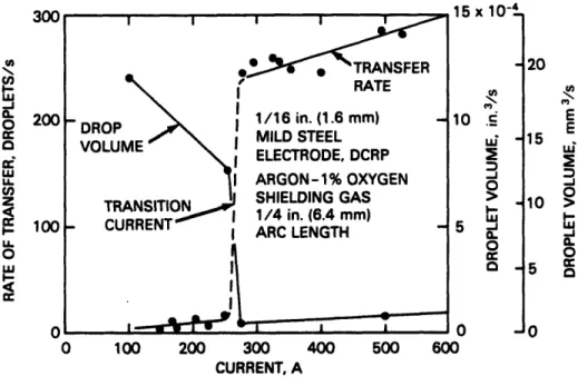
Another drawback to GMAW is that the transition from globular transfer to spray transfer is very abrupt as shown in Figure 4. If it is necessary to weld a seam at or near this transition current, a very erratic weld bead could result. Some research is currently being carried out to expand the range of the spray transfer mode [Jones et al, 1993] since it is generally a more desirable mode of mass transfer. By vibrating the feed wire the transition current can be reduced by as much as 20%, but a transition current still exists, and globular transfer occurs below this transition current.

,2

I-C

1-011

(15)

300 15 x 10. uJ "I o (L 0 uJ cc 200 100 O I I I ' DROP I VOLUME I TRANSITION CURRENT I * 'TRANSFER I RATE 1/16 in. (1.6 mm) MILD STEEL ELECTRODE, DCRP ARGON-1% OXYGEN SHIELDING GAS 1/4 in. (6.4 mm) ARC LENGTH I "r I I _ I C 100 200 300 CURRENT, A 400 500 600

Figure 4: Variation in Volume and Transfer Rate of Drops With Welding Current for GMAW

[O'Brien, 1991]

A larger scale negative effect sometimes experienced in all kinds of arc welding processes, including GMAW, is a phenomenon known as 'arc blow' which is when the arc and filler metal being deposited are deflected by magnetic forces induced by the current within the workpiece. In Figure 5 one can see that magnetic forces can be induced that vary with position of the torch. In the diagram below, there would be no deflection of the arc when the torch is directly above the workpiece lead and an increasing deflection as the torch is moved away from the workpiece lead.

10 5 N .=j_e Ui 2 0 I-w cc 0 20 E 15 E w ,J

r

0o 0 0 A - - - - -I -I I I ___ . I 15 X 10-300 i II

(16)

Debcted M etlTanbfr

M agnetd Flx Lies Defbcted

Pa

Co=et Path

w oif:

Figure 5: Deflection of Arc and Filler Metal From Induced Magnetic Forces

The limitations of GMAW typically apply to other forms of consumable electrode welding also. Although the mass transfer is stable and predictable in some operating conditions, it is erratic and hard to control in others. The lack of controllability over characteristics of the mass transfer and the limited independent controllability over both heat and mass flux into a weld seam is what motivated the development of the stream welding device described here.

_ _ _ -

-I>

(17)

B. Description of Stream Welder

A diagram depicting the process of stream welding in comparison to GMAW is given in Figure 6. This stream welder is essentially a small scale arc furnace with an exit orifice at the bottom of a crucible containing molten metal. During welding conditions, a molten metal stream emanates from this exit orifice due to the pressure in the molten metal chamber. By modulating the pressure within the molten metal chamber, one can control the velocity of the molten metal stream and hence, the mass deposition rate. To

stop the molten metal flow, the pressure in the molten metal chamber is reduced below some critical value where surface tension forces stop the flow.

Modulating the arc power in the molten metal chamber allows control of the

temperature of the molten metal stream. Since the pressure in the molten metal chamber and the arc power are independent, it is possible to control the temperature of the molten metal stream and the flow velocity independently.

With Stream Welding, not only are the temperature and rate of mass transfer

independent, but the forces acting on the molten metal stream are few in comparison to consumable electrode processes such as GMAW. Surface tension, gravity, and fluid forces of the shielding flow (momentum and viscosity) are still present, but

electromagnetic, electrostatic, and pressure forces generated by the evolution of gas at the electrode tip, have all been eliminated. The main factors affecting flow are the pressure driving the molten metal stream and the exit orifice geometry. This should lead to accurate control of both the rate of deposition as well as the location of deposition.

It is yet to be fully determined if modulating the temperature of molten metal stream will provide the necessary range of heat input to the weld. In chapter 4, this issue will be analyzed with both a mathematical model and through experimentation.

a. Control Systems

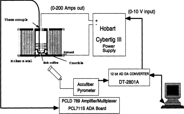
For precision operation of the stream welder it is necessary to develop a molten metal temperature controller, a molten metal replenishing system, and a stream flow rate controller. The former two have been designed and implemented as shown in Figure 7 and will be presented in detail in chapters 2 and 3.

The closed loop temperature control system uses a high temperature pyrometer for temperature sensing. The analog output from the pyrometry unit is digitized and

(18)

.JQ E co I II I' E k-I C a E U-c I ei I I A 3 5 U P o 8 a

I-CD

0)

c

E

Cu_a)

l)

4:5 a)

0-0)

ii cm c-C5

u

0) LL U -0 Aj

a

at 8 U 6) ...: - -- - - -:l::::::

(19)

o

CM 8 E a, E a)_en

c

a E

0 O

a, L0

(20)

analog signal dictates the current and hence the power into the furnace from the high bandwidth Hobart CyberTIG Im power supply.

The closed loop wire feed system is necessary to replenish the molten metal supply as it is ejected out of the furnace onto the weld seam. One of the most difficult aspects of this system is a means of sensing the molten metal level in the crucible. Presently the level is sensed by measuring the arc voltage which is proportional to the arc length. So if the molten metal level is low, the arc voltage is high. However, the voltage is also a function of the arc current that is being modulated by the temperature controller. Hence the voltage fluctuates with arc current. Another means of sensing molten metal level that was tried was measuring arc resistance, which is known since the arc voltage and current are known. It turned out that the arc resistivity is an even stronger function of arc current than the arc voltage which is why arc voltage is still the means of measuring molten metal level height: it has proven to do a satisfactory job for this stage in prototype development.

The arc voltage is preprocessed with a differencing amplifier and digitized. The digitized arc voltage is then incorporated into an on/off control scheme. If the voltage is higher than the reference voltage, wire is fed into the molten metal chamber where it melts from the heat of the surrounding metal. One of the main problems hindering the performance of this closed loop replenishing system is that the replenishing rate is relatively low. The wire cannot be fed any faster than the melting rate of the wire or it will eventually puncture a hole in the bottom of the crucible. The fact that the wire will melt faster at higher temperatures is accounted for in the on/off controller, at higher temperatures the wire is fed faster than at lower temperatures to improve performance where possible. The relationship between wirefeed rate and temperature is discussed in more detail in the molten metal level control chapter.

Before the flow control system can be developed, it is necessary to find an exit orifice material that can withstand the mechanical and thermal wear of a high temperature

molten steel flow. This problem is addressed in chapter 5 where two new furnace designs are presented.

b. Furnace Assembly

Most of the furnace assembly design was done by Steve Lee and a working

description of the first prototype is given in his thesis [Lee, 1993]. However, there have been a number of changes in this design to improve the performance of the furnace and to

(21)

cater to the molten metal temperature and replenishing control systems. AutoCAD drawings of the present state of the furnace assembly are given in Appendix A2.

As mentioned earlier, a high temperature pyrometer is used to sense temperature rather than a high temperature thermocouple (C type). There were problems with the noise as well as melting of the thermocouple at sensed temperatures above 1700 C. The

pyrometer is capable of reading temperatures up to 2000 C and can be upgraded to read up to 2700 C. To focus the pyrometer on a spot near the exit orifice, the opening in the base plate had to be enlarged. It was decide to have a "keyhole" geometry rather than a large circular hole to minimize heat transfer from the crucible to the surroundings. This keyhole shape allowed the pyrometer to focus on the crucible from an angle where it was less likely to be damaged from stray molten metal.

Additional insulation was added inside the furnace to help improve the maximum achievable temperature. Alumina felt insulation was added around the lower half of the molten metal chamber as shown in the cross section schematic. The felt is porous enough to allow the argon shielding gas to flow and perhaps even distribute the flow more evenly around the molten metal chamber causing a more uniform shielding flow around the molten metal stream. Additional insulation was also added below the crucible to reduce the effect of heat loss through the large keyhole opening in the base plate.

The wirefeed guide tube was angled to achieve higher wire melting rates which means better molten metal replenishing capabilities. The angled wirefeed improved wire

melting rates by more than 20%. This modification will be elaborated on in the molten metal replenishing system in chapter 3.

One significant operating characteristic that was changed was the operating arc voltage. This voltage was increased from 14-16V to 17-21V. The increased arc voltage increased the power input to the furnace which helped improve thermal performance. With the additional insulation mentioned above and the additional power input, the furnace was able to achieve temperatures well over 2000 C. The magnitude above 2000 C is unknown since the pyrometer cannot presently sense temperatures above this temperature.

The argon pressurization and shielding flow system was redesigned to improve control over the shielding flow. Initially, the Argon used to pressurize the molten metal chamber was also used as the shielding gas with the flow pattern shown in Figure 8a. The

reasoning behind this design was two-fold: the first reason was to ensure that the shielding flow was thoroughly preheated so it would not cool the molten metal stream.

(22)

there is negligibly more heat transfer away from the furnace and stream, but the shielding flow is now independent of the pressure within the molten metal chamber.

(23)

E s . ....l e .0 a S -I

I

\ $ ~~~~~:o 'U W cm A aL lYg v3

I

Ao

r-C) N4

0 0

(n O Cn: ._ I.I. 5

L.

US₁ A , : .: . .. | ,, :.: ..: . :.:'..:-:'

-o

CO

cn_, ._

C

LV) /

I

:::::::::::::;:::... ,>: i:!iii::: ... :c::::::iF:·:·:·: :i:i:i :·1:·:·:·:·:·i: 1 ,,,ji:·1:·: ·.·.·.·.·.·.·.·;.·.·.· ·.·. :i:i:i:R:S ·;·.·.· ·:;:·:··:·:·:·:·:;:·:;:;'·'·'·..·. J_I, p) .·.·.·.·.·.·.·.·.·.·.·.·.·.·.·:·"""' .·.·.·.·.·.·.·.·.·.·.·.·.·.·.·.·.·.·.·.· r, .·.·.·;·;·;·.··s zr;;r·;·;;·.s.. :::j::::::SI:::j:2_{· ·}_{:·:·u::::::::::n::::mas U} :::::5:·::::·:·.·; ::::: .·;· ::::::: i:::: ''''''' ·.·.· ::::::: I ''''''' '''' ::::: ·.·.._·'''''' ··· .·.·.·.·.·.·.·.·.·.·.·.·.·.·;.·.·.·:.·.· .·.·.·.·.·.· ·.·.·.·.·.·.·.·.··n··....;r;·;·;·..;..;·;·; .·.·.·.·.·.s.·...·.·.·.r ... ·.;·.·.·.·.·. ·.·.·.;· _g )::'::5:: :::::i'I:·:';'2-'' ··· :.··.·.·.s·X·"·'":.:·:·:.: .·.·.·.·2.·.·.·...·.·.;·.·. ·.·..·. :::I:::::!:I:::1::R:::::::::::::::·

i

.·.·.·.·.·.·.·.;·.·.s;;·.;·.·.·:.·.·;.·.

(24)

Chapter 2: Closed Loop Temperature Control System

A. Overview

Controlling the temperature of the molten metal being ejected from the stream welder is one of the primary objectives in developing this device. By controlling the

temperature of the ejected molten metal, we control the heat flux into the weld seam; this, in turn, determines certain properties of the weld seam (i.e. penetration depth, heat

affected zone, etc.). A schematic of components of the temperature control system is shown in Figure 9.

(25)

Nomenclature:

T - Temperature [C]

t - Time [seconds]

Vpyro - Pyrometer output voltage[V]

lout - Current output of Hobart Power Supply[A}

Varc - Arc voltage[V]

Pin - Power input from Hobart power supply [W]

l1 - Arc efficiency

Vinput - Voltage input to Hobart Power Supply[V]

K1 - Generalized thermal mass coefficient[J/C]

K2 - Generalized convective heat transfer coefficient[W/C]

Ka - Steady state relationship between Pin and T[C/W]

Ta - Time constant for the first order approximation of

plant[seconds]

To implement a digital control system with a PC, the analog temperature information from the thermocouple or pyrometer must be digitized. The signal from the pyrometer is 0-10 volts and is related to the sensed temperature by the following function:

T=500C + V 1500C

10[V]

The 0-10 volt signal is digitized by a 12-bit DT-2801 A/D D/A board and read by the program pyropid.c. To filter out some of the noise in the pyrometer signal, this program acquires 10 voltages and averages them over a time interval of about 0.03 seconds. When accounting for the execution time of the rest of the code, which also controls the wire feed rate, the resulting sample period is 0.1 seconds. The filtered temperature is then used to compute the closed loop control action with a PID control algorithm. The digital control action is then converted to an analog signal (0-lOvolts) with a D/A channel on the DT2801. This analog signal (0-10 volts) is sent to the Hobart CyberTIG III power supply where it dictates the current and hence the power into the furnace. The current out of the Hobart is related to the input signal by

(26)

Pin = ' Iout Vac

Here Tl is defined as the arc efficiency. The time constant of the Hobart power supply is

roughly 0.001 seconds, negligibly small relative to the plant thermal time constant which is why its input/output relationships are treated as static as given in the above equation.

B. Temperature Sensing: Thermocouple Versus Pyrometer

Temperature information can be acquired using either a high temperature thermocouple immersed in the molten metal chamber, or a high temperature pyrometer focused near the crucible exit orifice. There are advantages and disadvantages to both methods. The obvious benefit of using thermocouples is the relatively low initial cost, the tungsten rhenium thermocouples cost approximately $100 each (including lead extensions etc.) and the amplifier mulitplexer board (Omega PCLD 789) for processing the thermocouple signals is about $250. The Accufiber 100C pyrometer unit, on the other hand, costs roughly $6000. Neither of these prices include the A/D boards.

Since both were readily available in the LMP, both were initially incorporated in the temperature control design to see which would work best. The tungsten rhenium thermocouples worked well until the furnace was improved to a point where it could achieve temperatures in excess of 1700 C, the thermocouples started to melt at these high temperatures. These C type thermocouples are rated for a temperatures in excess of 2400 C, but this is only in an ideal inert atmosphere. Although argon is used as the

pressurizing gas, other materials such as carbon, molten steel and trace amounts of oxygen may be reacting with the tungsten rhenium alloy. Putting the thermocouple in a zirconia test tube to keep it isolated from some of these substances did not help, the thermocouple still melted within the test tube. It is yet to be determined if the

thermocouples are faulty or if a significant amount of oxygen is in the test tube. In any case, this meant that the thermocouples could not be used for closed loop control above 1700 C.

The main advantage of the pyrometer is that it is non-intrusive and hence is not directly exposed to the high temperatures within the furnace. It relies only on the infra-red

radiation collected from the object on which it is focused to measure temperature. The focal length of the Accufiber 100C is 30cm and the desired focal point is the base of the crucible, next to the exit orifice. The temperature at this location is less than the

(27)

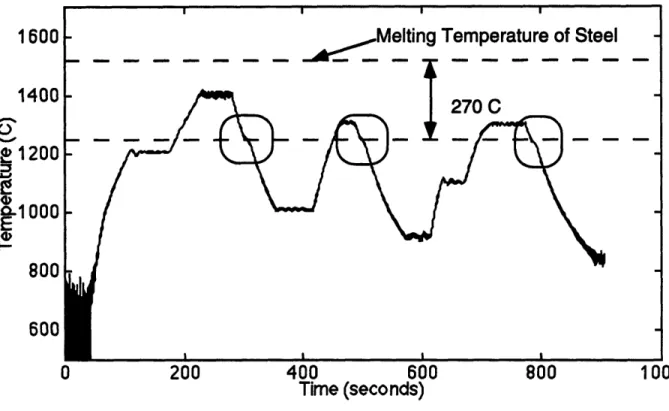
temperature within the molten metal chamber, the difference between the molten metal chamber temperature and the sensed temperature can be approximated using the following closed loop temperature response.

1600 1400 )I I 1200 a.,

0-1000

800 600 0 200 400

60

U800 Time (seconds)

Figure 10: Determination of Difference between Pyrometer Sensed Temperature and Actual Temperature within Molten Metal Chamber

(from step4894.dat)

The three circled parts of the plot most likely represent the solidification of the molten metal. Since the solidification temperature of the steel is about 1530 C it appears that the difference is about 270 C. At higher temperatures this difference between the molten metal temperature and the sensed temperature is likely to increase since temperature gradients would expectedly increase with temperature.

The reason the pyrometer is not focused directly at the exit orifice is because of the difference in emissivities of the molten steel and graphite. To sense the temperature accurately, the emissivity of the material must be known and programmed into the pyrometer unit for it to compute for temperature. The emissivity of molten steel is 0.45

(28)

--temperature measurement would change depending on whether or not molten steel was flowing.

Presently, the Accufiber Pyrometer can accurately read temperatures between 750 C and 2000 C, the upper limit on this range can be increased to 2700 C with a $1000 upgrade. Between 500 C and 750 C, the signal is extremely noisy, but this temperature range is of little interest.

Because of its higher temperature capabilities and upgradability, the Accufiber Pyrometer, rather than tungsten rhenium thermocouples, is used for the closed loop temperature control system. The thermocouples are sometimes used for lower temperature (less than 1700 C) data acquisition.

C. Temperature Dynamics of the Furnace

a. Defining the Plant

Ultimately it is desired to control the temperature of the molten metal stream by modulating the power input from the arc. In this section the focus is to determine a suitable input output relationship that accurately describes the thermal dynamics of the stream temperature in relation to the power input.

The stream temperature will be directly related to the crucible and molten metal temperatures. Figure 10 in the previous section indicates the temperature in the molten metal chamber might be significantly higher than the sensed temperature of the exterior of the crucible, and the temperature of the stream will likely be between these two temperatures. Before entering the exit orifice, the molten metal will be the same

temperature as the surrounding molten metal, but while passing through the exit orifice, there will be some cooling of the molten metal. The resulting temperature of the

emanating metal will be a function of relevant states such as flow rate, as well as temperature of the molten metal chamber and the temperature of the crucible. It should be noted here that there will be some heat transfer away from the molten stream after exiting the exit orifice and before it hits the workpiece due to both radiation and

convective heat transfer. These effects will be minimized by minimizing the distance the stream has to travel and hence, will presently be neglected.

Ideally, an estimator could be formulated to predict the emanating stream temperature given the relevant furnace states. However, formulating this estimator would lead to complicated analysis and experimentation, so as a first attempt, a more simplistic approach will be taken. The approach will be to control the sensed temperature, that of

(29)

the base of the crucible, rather than the stream. From initial observations of open loop temperature responses to steps in input power, it appears that the system behaves much like a first order system, which indicates that it is possible to use the following equation to describe the plant dynamics:

K,=-K2T+ Pi. (1)

Here K 1 is a generalized thermal mass coefficient and K2 is a generalized convective heat transfer coefficient. Both of these coefficients will be functions of temperature but for now are treated as constants. Taking the Laplace transform of eq. 1 gives the continuous transfer function describing the simplified furnace dynamics:

H(s) T(s) K,

Pi,(s) TsS + (2)

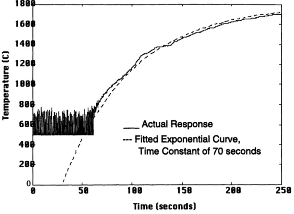
Both Ka and 'a can be determined experimentally from open loop responses to various step inputs of power. One such response is shown in Figure 11. The dashed line, which is a first order exponential with a time constant of 70 seconds, fits the response

reasonably well. However, such large step responses are not of as much concern as small steps at elevated temperatures, since this will more closely resemble an actual stream welding situation. These types of open loop responses are looked at later in this chapter.

(30)

16081 1481 1281 m 1881

mI

481 281 I /'

I~~

_I~~O

I

Actual Response

e:. uL_I t_ _ _m .... _.. .LI _ .. _.

// --- r-lea txponenial urve,

, Time Constant of 70 seconds

f

0 58 100 158 288 258

Time (seconds)

Figure 11: Open Loop Temperature Response Depicting First Order Furnace Dynamics (from feed512.dat)

b. Variations in the Plant Dynamics

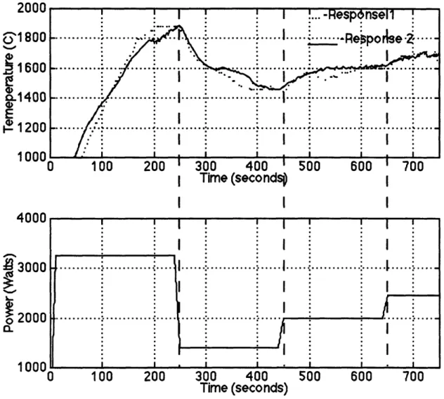
The open loop responses do not always display the almost ideal first order behavior shown in Figure 11. It has been found that there is variation in open loop responses obtained under the same experimental conditions. Figure 12a shows two responses that are subject to the same experimental conditions. The power input as a function of time for both responses is given in Figure 12b. Both experiments are carried out using the same mass of molten metal, approximately 60 g. Although these responses are similar, there are some definite differences. These differences, such as the one that occurs for the dashed line response at about 520 seconds, are not easy to explain. It could be nature of the heat source, the resistivity of the arc may fluctuate in an unpredictable manner or it could be problems with the pyrometry unit.

l

co

I

(31)

ii nfn

Q

a} 64 A. 4) 0 E 4)

4000

!I

t

3000

C

. . ...

...-...

i...I....·

1 ·.

.

ooo

2000

...

· I *I · I I 1000 0 100 200 300 400 500 600 700 Time (seconds)

Figure 12(a) Two Open Loop Temperature Responses Carried Out Under the Same Circumstances with a Molten Steel Charge of 60g,

Temperature Sensed from Base of Crucible with Pyrometer 12(b) Power Input as a Function of Time

(from weld712.dat and weld714.dat)

Both Ka and t a were found experimentally from open loop step responses in power input, like the ones shown in Figures 13 and 14. As expected, Ka and :a varied under different operating conditions such as different molten metal masses and temperature ranges. However, some of this variability can be attributed to the erratic behavior

(32)

approximated steady state temperature by the steady state power input as given by the equation below.

Ka =limso. s+ = lim" Pn(t)

It was found that ra varied from 30 seconds to 90 seconds depending on the operating temperature and amount of metal within the molten metal chamber. The value of Ka also varied anywhere from .6C/W to .89C/W. Two open loop responses are given in Figures 13 and 14. An exponential response is fitted to each response at t = 250 seconds. In Figure 13 the amount of molten metal is 50g and in Figure 14 the amount of molten metal is 80g. The value of ta in Figure 13 is 30 seconds and for Figure 14 it is 80 seconds. 1800 e 1600 1400 1200 100 1 200 1 300 400 1 500 600 1 700 I I Tike (seconds) I I I I I 800 900 1000 1nrm 0 100 200 300 400 500 600 700 800 900 1000 Time (seconds)

Figure 13 (a) Open Loop Temperature Response to Steps in Power Input, Molten Metal Charge is 50g, Temperature Sensed from Base of Crucible with Pyrometer;

(b) Input Power vs. Time (from weld617.dat) 0 O lnAn 4000 A 3000 . 2000 vvv

(33)

. E

0--4000

% 3000

-2000

0 1000

0 O n 0 200 400 600 800 1000 Time (seconds)

Figure 14 (a) Open Loop Response to Steps in Power Input, Molten Metal Charge is 80g Temperature Sensed from Base of Crucible with Pyrometer;

(b) Input Power vs. Time (from weld6172.dat)

Although there is substantial variation in both Ka and ta both are initially given nominal values of ra=5 0 seconds and Ka = 0.6 C/W. Appendix E analyzes of the effects of operating conditions on Ka and ra. The transfer function that will be used to describe the temperature dynamics of the stream welder is as follows:

T(s) =.6

H(s)= T = *6

s)

P(s) 50s + 1

It turns out that these nominal values work well in designing the closed loop

(34)

D. Control System Design

With the plant description from above it is possible to begin designing a controller. In choosing a control scheme it is necessary to eliminate any steady state error. To achieve this, integral control action must be used since this is essentially a type 0 system (no poles at the origin of s plane). With these criteria and simplicity in mind, either a proportion plus integral (PI) controller or a proportional plus integral plus derivative (PID) controller will be used. Ideally, a PID controller would not be necessary since a PI controller can arbitrarily place the closed loop pole for a first order system. However, derivative control action may help to minimize temperature disturbances.

a. PI Controller

First the option of a PI controller will be analyzed using root locus analysis and then simulation. To carry out the discrete root locus analysis we must first find the discrete equivalent (using zero-order hold reconstruction) of the continuous plant transfer function. The equivalent is given as follows:

Ho = Lz{L} =~s .0012

Hq(z) z - I Z{H(s) _ (1.6)

z S (z -. 998)

The PI controller is of the following form:

Gp, (z) = Kp(1 + T()) (1.7)

The sampling period T may range from 1 second to 0.01 seconds in the future. The sampling period will never by any faster than 0.01 seconds with the present pyrometer because its maximum sampling frequency is 100 Hz. Ultimately the sampling period will depend largely on the other tasks required of the C program controlling the whole system which will have to cater to the other control systems as well. Presently, the program is doing free running A/D D/A conversion that results in a sampling period of

approximately .1 second. The value of Ti was initially chosen to be 2 seconds since a lesser value would make the system very sensitive to the sample period. With the z transforms of the plant and the controller defined, one can perform some root locus analysis to find the best Kp given T and Ti above. The characteristic equation of the closed loop system is

(35)

GcpiHeq(Z) = 1 + Kp 0012(1.05

-(z- .998)-(z- 1)

The resulting root locus is shown in Figure 15

1 0.8 0.6 0.4 bO .M onW 0.2 0 -0.2 -0.4 -0.6 -0.8 -1 1 -0.5 0 0.5 1 Real Axis

Figure 15: Discrete Root Locus for PI Controller

Kp=148 corresponds to the break-in point on the real axis at z=.909. Ideally, from the standpoint of root locus, we would choose a Ti that is slightly more than T which would result in a break-in point close to the origin with the appropriate Kp, giving a very fast response with no overshoot. Designing this control system would be unrealistic though, it would require an enormous amount of power and the maximum available from the Hobart is only 4000 Watts.

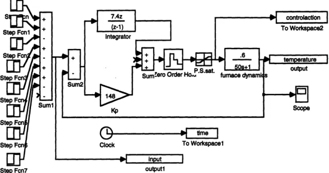
A better means of design in this case is through simulation, a block diagram of the

I - I l I

i

I . . L . . . .

(36)

Step Fcn7 outputl

Figure 16: Block Diagram of PI Controller

All of the simulations have multiple step inputs since this will be similar to the anticipated mode of operation when welding.

Some important features of the system should be noted here. One feature is that we are only able to put heat into the furnace and cannot take it out, this characteristic is accounted for in the saturation block. The minimum heat input is 40 W while the

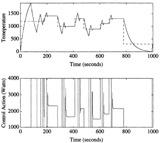
maximum is 4000W. The minimum is 40 rather than 0 because it is necessary to sustain the arc throughout the process; a current of 0 would extinguish the arc and require restarting it with the high frequency arc starter which can sometimes cause the computer to lock up. To obtain a controlled negative energy input, one could incorporate a cooling system, but this is presently deemed unnecessary since the furnace dissipates a substantial amount of heat at operating temperatures. The simulated step response of the system is shown in Figure 17. The reference input is given by the dashed line and the simulated response is given by the solid line. This response shows substantial percent overshoot even though the chosen gain value placed the closed loop root locus poles on the real axis. This discrepancy can be attributed to the saturation of the power supply which cannot be accounted for using root locus analysis.

(37)

1 An IJUU

1000

500 0 200 400 600 800 1000 Time (seconds) A f'mf%" 3000 .o 2000 0 0 200 400 600 800 1000 Time (seconds)

Figure 17: Simulated Response of Root Locus Designed PI Controller

There are a number of ways to improve this response. One would be to pick a larger Kp and a larger Ti, this would place less emphasis on the integral control action which is causing the overshoot. Another way that would have a similar effect, is to incorporate an anti-windup feature which limits the magnitude of the error within the integral. In other words, it would limit the magnitude of e' in the following equation representing the control action

uc(t) = Kp(e(t)) + P e' (t)dt

Both of these options are incorporated into the PI control scheme and tuned iteratively. T]he closed loop response improved substantially as shown in Figure 18 below. The value of Ti was increased to equal Kp and Kp was increased to 1300. The anti windup limits were fixed at (+/-)100 C.

(38)

1 Cl 10C aS Time (seconds) ig 0 8 U 0 0 ru. 0 200 400 600 800 1000 Time (seconds)

Figure 18: Simulated Response of Refined PI Controller

b. Design of PID Temperature Controller with Anti-windup

Even though this PI controller performs well, the control system might be further improved with respect to temperature disturbance rejection by using a PID controller while retaining the anti-windup feature. Disturbance rejection will likely be important to the control system given the slightly erratic nature of the open loop temperature responses given in Figure 12. The PID control law is of the following form

Tz TD(z- 1)) G,(z)= Kp(1 + 1 TZ T(z - 1) Tz

K + Kz + K(z- 1)

(Z (-1) z

The first approach in tuning this controller was to use the Ziegler-Nichols method which uses an open loop transient response to determine initial values for Kp, Ti, and Td (or Kp, Kd, and Ki). The method is depicted in Figure 19

(39)

4.. M

a-3

0

a) L E a) C t* I t d Time (seconds)

Figure 19: Necessary Parameters for Ziegler-Nichols Tuning of PID Controller

How to calculate Kp,Ki and Kd, given the parameters described in the previous figure, is shown on the following table [Ogata, 1990]:

It should be noted here that td is actually 0 since the behavior of the system is first order but here it was assigned to be 0.1 seconds, a very small value relative to the plant time constant. This was done since it is necessary that td be some finite value to use this method, and no alternative methods were found. The value of R was obtained from open loop responses and is 66.7 C/sec. Given these values of td and R, the resulting values of Kp, Ki, and Kd are shown in the table above. These values serve merely as starting points in determining the best values of Kp,Ki,and Kd. Taking Ki and Kd from above, the resulting root locus as a function of Kp is shown in Figure 20.

Controller Kp Ki Kd

Parameter

Parameter Formula 1.2/(R*td) (Kp*T)/(2*td) (Kp*.5*td)/f

Resulting Parameter 1333 667 667

(40)

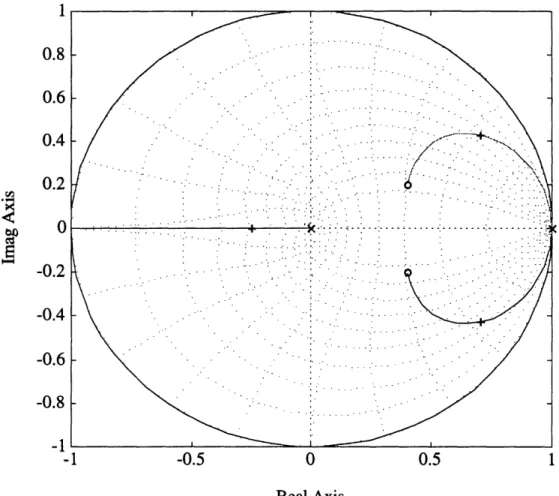
1 0.8 0.6 0.4 0.2 0 -0.2 -0.4 -0.6 -0.8 -1 -1 -0.5 0 0.5 1 Real Axis

Figure 20: Initial Root Locus for PID Controller

One can see that the root locus predicts a oscillatory response which turns out to be the case as shown in simulated response in Figure 21

r Z . | -i' * \ 6 6 \ |, + + \ * + | -' ' ' ' + ' \ . * * ' ' . . , w \ . , * , * \ \ 4 * , ^ . + , + \ '. " '. + ..' . * ''" ' + " . . " \\ 6 F F s + \ . \ e , . * 6 . . . w \ S v vo \ _ , , e ,, /+ , u ss \ / * , 6 6 ^ ,/ w ' , \ \ \ \ *-' . * 1 ' * *. * ' * 6 - - -, ,\E * * 6 s s + e e t . . . t . . * ' > . ' @ | J " ^ ' ' J . * * w . ' ' ' ' ' ' | + we ' ' ^ ,' .' +' ' ' ' ' . * z v .-4 - ' ' * " ", > . -- } : " .l ' ''-. .' 9 WF '' " ' " | 's * . @ . ., b , .- - -.\ -\ , 4 . . o - ./ : ./ 1+ I * , ; ,,, ,, \' , \ ' ', + / I | e b . \ , \ S / / ''I ' ' ' ' '* ' ' ' .' _ / / / . . . . / S S . . . S 'l . . .* * ' ' S . ' @' ',.6 6-,+,. ' '- . f-'.' . . // ,, s . , , + + / | + w / "- . ' b ' ,' / . . @ . . , . + / '' '' '' o | . / s / z S e S I i

~~~~~~~~~~~~~~~~~~i-·.·

_ J I N". VID ".10 It .9 I 1

(41)

4)

F-0 200 400 600 800 1000

Time (seconds)

Figure 21: Simulated Response with Initial Values for Kp, Ki and Kd

Using root locus analysis, the value for Ki was decreased to bring the closed loop zeros onto the real axis and dampen the response. Ki was further tuned iteratively using simulation, until a value was found that gave a suitable response (Ki=l). Better values for Kp and Kd were found in a similar fashion (Kp=1300 and Kd=500). The block diagram of the final system is shown in Figure 22.

(42)

Step Fcn7 outputl

Figure 22: Block Diagram of Final Design of Temperature Control System

The performance was greatly improved from the response shown in Figure 21, as shown in Figure 23. The overshoot appears to be less than 10% for even the large initial step to 1200 C where there is some integral wind-up. The main concern, however, will be the smaller steps like the one from 1200 C to 1400 C since this will be the more likely magnitude of control steps when welding.

(43)

I £Lf^

U

F-0 200 400 600 800 1000

Time (seconds)

Figure 23 Simulated Response of PID Controller with Anti Wind-up Feature

In comparing the performance of this PID controller with the previous PI controller, it turned out that there was little, if any, benefit in adding the derivative control. In many situations derivative control action is incorporated in furnace temperature control systems to help reduce disturbances, but in this case it had no apparent effect on disturbance rejection. Both controllers were subject to simulation with both white noise and step temperature disturbances at the output, and there was no observable difference between the two controllers. However, the PID controller will continue to be used since it has no negative effect on the system.

c. Performance of Actual Controller

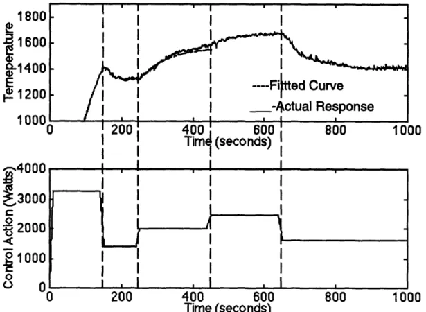
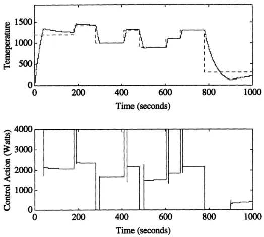
We now compare this simulated response with reality, implementing the same values of Kp, Ki, and Kd in the c code, pyropid.c, that were determined from the simulation. The actual response is shown in Figure 24.

(44)

1600 1400 G 1200 1000 800 600 dAnn 0 200 400 600 800 1000 Time(seconds)

Figure 24: Actual Response of Closed Loop PID Temperature Controller with Anti Wind Up Feature

(from step4894.dat)

The actual response is similar in to the response predicted by simulation in many

respects. It appears that the actual response has a larger time constant than the simulation which can be attributed to more molten metal within the crucible. The actual response appears well dampened with very little overshoot. There is some negligibly small steady state oscillations in the response, but the system can be fine tuned when a high degree of temperature precision becomes an issue. Overall the performance of the PID temperature controller is good at this stage in development of the steam welder.

(45)

Chapter 3: Closed Loop Molten Metal Level Control System

A. Overview

For the stream welding process to run continuously, it is necessary to replenish the molten metal supply as it is ejected out of the furnace and onto the weld seam. Another reason to maintain the molten metal at a constant level is to ensure a consistent thermal mass for the temperature control system. The method used to accomplish a constant level is a wire feed system. Solid wire is fed into the crucible where it melts from the heat of the surrounding molten metal. A schematic of the components of the molten metal level control system is shown in Figure 25:

Wire i I I I I I

Arc Molten Metal Flow

I I

Figure 25: Components of Closed-Loop Wirefeed System

The variable of interest is the height of the molten metal in the crucible, H, which should be maintained at a constant level. The state of this variable is sensed indirectly by measuring the arc voltage V. The arc voltage is proportional to the arc length h. Since the

I

I : I II

(46)

and negative electrodes of the power supply. Since the arc voltage will range anywhere from 10 to 25 volts, it is necessary to preprocess this signal to get it in a range that the DT 2801 A/D board can handle (0-10 volts). This is accomplished with a simple differencing amplifier with a gain of 0.24. The signal from the differencing amplifier is digitized by the DT2801A board. This digitized value of the arc voltage is then divided by 0.24 and incorporated into the control scheme.

The control scheme is essentially an on/off type that is implemented with the C program pyropid.c. One important aspect of the system is that the maximum wirefeed rate is limited by the melting rate of the wire being fed into the crucible. It is important not to feed faster than the wire can melt to avoid damaging the graphite crucible from steel wire poking into it. To prevent this kind of damage, the control scheme uses the sensed temperature in determining the magnitude of the 'on' control action, higher sensed temperatures mean that a higher wire feed rate can be used without damaging the

crucible.

The control action is computed every 0.1 seconds and sent to the DAC. The analog signal from the DAC is sent to the modified NA-SR wire feeder. Here the DAC input voltage is directly proportional to the steady state wirefeed rate (0-10 volts=0-70cm/sec). The fed wire then melts in the crucible, replenishing the molten metal supply.

B. Modeling the Dynamics of the Wirefeed System:

Before coming up with a suitable control strategy it was necessary to understand the dynamics of the system components mentioned above as well as the nature of the disturbances to the system. A continuous block diagram of all of the main system components is shown in Figure 26.

(47)

Temperature

r

I I 1+ I I I I ible h I I

_L_______Differe ncing Amplif ier

Computer with ADC & DAC

Figure 26: Block Diagram of Closed Loop Wirefeed System

Here an explanation is given of how the transfer functions for each component was obtained. Most are simple static functions.

The transfer function for the wire feeder is essentially that of a typical velocity controller. It was obtained from an open loop response to a step input in voltage and observing the wirefeed velocity response. This had already been done by Hale [8] who used the same wire feeder (but less modified) for some of GMA Welding research. Both the motor time constant of 0.1 seconds and gain of 70.4mm/sec/volt, determined by Hale, were verified.

Kv will be dependent on the diameter of the wire fed into the furnace since it

translates wire velocity into a volume flow rate. The relationship between these two is as follows

volume flow rate=(wirefeed velocity)*x(Rwire)2

So the resulting Kv is:

Kv=t(.00045m)2

(48)

rate into the crucible is the wirefeed volume flow rate minus the outflow from the

crucible. The relationship between this net mass inflow rate and the molten metal height is given here (it should be noted that the slight slope of the crucible wall is unaccounted for here)

dVI = R2cicbe dh

dt dt

1

h(s) = _s 1_R2_cnicible

The height then translates into an arc voltage, this relationship should be similar to the relationship between arc voltage and arc length for a TIG welding process. The possible problems with determining the height by sensing the arc voltage is that the arc voltage is also a function of arc current which fluctuates with the temperature control action. It is also a weak function of the temperature of the argon as well as the concentration of metal vapor in the arc. However the arc voltage is primarily a function of arc length and will be initially be assumed to be linearly related to arc length as the proportionality block Kr indicates. A suggested alternative was to measure the molten metal level by measuring R since both V and I are known. It turns out that R is even less reflective of height, being highly dependent on the arc current. This is apparent when the current is doubled from 100 A to 200 A, at 100 A the arc resistance is 0.16 ohms and at 200 A its 0.095 ohms. On the other hand, the voltage only changes from 16 V at 100 A to 19 V at 200 A. The value of Kr was found experimentally. The measured arc length of 4 mm resulted in an arc voltage of 13.8 Volts. Hence Kr is roughly 3.44 Volts/mm.

The differencing amplifier was constructed of a +-15 volt power supply, an LF741 operational amplifier, and some accompanying resistors. The dynamics of the amplifier can be neglected since its bandwidth is orders of magnitude higher than the rest of the system. A schematic of the amplifier is shown in Figure 27, its gain is 0.24.

(49)

+15

Vout

Rf=14.8KOhms Ri=61.5KOhms

Vl=Positive electrode voltage V2=Negative Electrode Voltage Vout=Voltage out to ADC

Figure 27: Differencing Amplifier for Arc Voltage Sensing

The block in Figure 26 which has the biggest effect on the performance of the system is the saturation block. As mentioned before, the maximum melting rate of the wire limits the maximum feed rate. To verify the damaging effect on the crucible, when feeding faster than the melting rate of the wire, a experiment was carried out where the wire was fed faster than the calculated melting rate. The temperature was maintained at

1800 C and the wirefeed saturation limit was fixed at 9.8 cm/sec, well above the 7.7 cm/sec melting rate. The arc voltage was initially at 20 when the level controller was activated, the reference voltage was set to 18 volts. The wire fed for a couple of minutes before the wire poked through the bottom of the crucible. This verified that the wirefeed rate should not exceed the melting rate of the wire. Because of this wire melting rate limitation, the wire feeder cannot replenish as quickly as the molten metal is ejected unless the ejection rate is very low (less than 19 mm3_{/sec at 1650C). It should also be}

noted here that the lower saturation limit is 0 since no negative control action is possible, this is due to the fact that mass can only be added and not withdrawn with the wire feeder. Because of the nature of this saturation, a simple on/off controller is used; something like a PID controller wouldn't improve the performance because of the upper saturation limit which is now discussed.

(50)

T - Temperature of the feed wire (K) Tmm - Temperature of the molten metal (K)

OE -T-Tmm

E - Energy (J)

t - Time (seconds)

h' - Generalized convective heat transfer coefficient (11,627W/m2K from experiment)

p - Density of feed wire (7800 kg/m3₎

c - Specific heat of feed wire (434 J/kgK) ro - radius of wire (.45mm)

As - Surface area of wire immersed in molten metal (m2) V - Volume of wire immersed in molten metal (m3₎

r - Radial coordinate of wire x - Axial coordinate of wire

k - Thermal conductivity of mild steel (60W/mK) a -k/pcp (18xl06W/mhn2 )

H - Height of Molten Metal (1cm)

The maximum wirefeed rate is dictated by the maximum rate at which the solid steel wire melts when fed into the molten metal bath. This wirefeed rate will be a function of the temperature of the molten metal, at high temperatures the melting rate will be faster which allows higher wirefeed rates without risking damage to the crucible. To get an estimate of the melting rate, some heat transfer analysis was carried out that predicts the melting rate at various temperatures. A schematic of the problem parameters is shown in Figure 28.

Molten Metal

H

(51)

Figure 28: Parameters in Analyzing Wire Melting Rate

The Problem was approached by finding the time t that it takes to melt a wire segment of length H and then dividing H by t to get an approximation of the maximum wire feed rate. The diameter of the wire is D and it is at an initial temperature Ti before immersion in a molten metal at temperature Tmm. Two methods are used to determine the time t, the lumped capacitance method or, more accurately, solving the appropriate form of the heat equation which accounts for multidimensional effects. Both methods have

convection as a boundary condition. The convective heat transfer coefficient, h', was determined experimentally at one temperature and assumed to remain constant for the range of analysis temperatures. It should also be noted that latent heat effects are accounted for in the convective heat transfer coefficient as will become apparent when explaining how the value for h' was determined. Each method gives similar results in predicting the wire melting rate as will be shown.

a. Lumped Capacitance Method

The time t can be calculated using an energy balance as follows:

h'A (T -Tmm) = pVdT dt

Here the change in internal energy of the wire segment is proportional to the heat flux across the wire due to convection. By letting O=T-Tmm:

pVc dO -8 h' A dt

Separating the variables O and t and integrating yields:

pVc ine = t

h'As f

Of is defined as the molten metal temperature minus the melting temperature of the steel, and Oi is the molten metal temperature minus the initial temperature of the wire segment. The only unknowns are h' and Oi. The value of Oi will be highly dependent on the

(52)

experimentally based on this assumption. These values of h' and Oi will be used in subsequent calculations in determining the maximum wirefeed rate for various

temperature ranges. In experimentally determining h' the temperature was held constant at 1650 C while I manually feed a 300mm length of wire as fast it melted (this was apparent from continually hitting the bottom of the crucible). The time to feed a segment of this length turned out to be 6 seconds. Hence the resulting maximum wirefeed rate is 50.8mm/sec at this temperature, and the value of h' is 11,627W/m2K (assuming Ti is 500 C).

With the values of h' and Oi as given above it is possible to estimate the maximum wire feed rate at various temperatures by simply dividing H by the expression for t given above. Using this lumped capacitance analysis the maximum wire feed rate at 1800 C is 7.7 cm/sec, at 2000 C it is 10.36 cm/sec and at 2200 C it is 13 cm/sec.

b. Accounting for Spatial Effects

To reinforce the lumped capacitance results the same problem will be solved using a more rigorous method that accounts for transient conduction in the r and x directions . Figure 29 shows a segment of wire immersed in the molten metal, again we want to find the time t after the segment is submerged when point T(O,H) reaches the melting

temperature of steel.

T(O. H.t) I I

Tr Ml

if orm

Figure 29: Schematic of Wire Segment Immersed in Molten Metal

(53)

1 aar a2T 1 aT

r ar) 2 =a

-A closed form solution of this partial differential equation can be obtained using the separation of variables technique. The result may be expressed in the following form [Incropera and Dewitt, 1990]:

T(r,x,t)-

Tmm

t)

m

l

T(r,t)-

Tmm]

Ti - Tr = 7 - TMm semi-inf inite Ti- Tmm _infinite

solid cylinder

So the two-dimensional solution is expressed as a product of one-dimensional solutions that correspond to a semi-infinite solid wall and an infinite cylinder with the same radius as the wire.

The one dimensional semi-infinite solid solution is given by the following (erf denotes the Guassian Error Function)

T(x,

t)- Tr

_'

=-~'"

_=-[erf-_'1ei

X

-

t

_erf-

(

ht4 '

+h- ]

TiJ-T semi- infz 2ie 224

L

;i

k

solid

The approximate graphical representation of this function is given in [Incropera and Dewitt, 1990] and is shown at the end of Appendix D. The graphical solution only requires the following dimensionless coefficients:

k and

x

The one dimensional infinite cylinder solution is given by the following:

[

T(t)-T

]infinit

=Cnexp(-2Fo)Jon

(54)

2 _ J_ _ _

c, =T.

j2(¢)+j2g,)

Here J 1 and Jo are Bessel functions of the first kind and the discrete values of In are the positive roots of the transcendental equation

Bi- Jo(Cn)

A graphical representation of the infinite cylinder solution at r=0 is given in the heat transfer text [Incropera and Dewitt, 1990] and also provided at the end of Appendix D. This graphical solution requires the inverse Biot and Fourier Coefficients which are as follows k 17-Bi' = = mK hr2 1 1,6 2 7 -- .00045m m K 2 4.2x10 - t at seC Fo = (.00045m)2

The value of t was solved for recursively and the results agree fairly well with the lumped capacitance method. At 2200 C the answers from each method differed the most, the lumped capacitance predicts a t of 0.078 seconds and the more rigorous method predicts a t of 0.099 seconds. Dividing H by these times yields maximum wirefeed velocities of

13cm/sec and 10cm/sec.

D. Control Scheme

Since the main factor limiting the performance of the level control system is the melting rate of the wire, the control system uses the analysis above and changes the wire feed saturation limits as a function of temperature. If this temperature feedback were not incorporated, the wire feed rate would be limited to the maximum wire feed rate at the lowest operating temperature. The wire feed rate as a function of temperature used in the C program pyropid.c, is given below:

T. - 1650 cm cm wirefeedrate = m-1650.cm + 3 cm

(55)

The wire feed rate is slightly less than the maximum calculated melting rate to allow for some margin of deviation between the calculated maximum melting rate and the actual melting rate. This measure of safety is incorporated because when the feed wire punctures the crucible a dangerous situation results, molten metal flows uncontrollably out of the furnace. Another safeguard incorporated in the program pyropid.c is that the system will only feed wire if the furnace temperature is above 1650 C.

To analyze the performance of the molten metal level controller, simulations were carried out using Simulink. Analysis techniques such as root locus are not easily applied given the saturation nonlinearity that has such a big effect on the system. The wire feeder will only be able to maintain a constant level if the flow out is less than the mass flow in from the wire feeder. At 1650 C the outflow should be less than 19.6 mm3/sec, for the wire feeder to maintain a constant level; and at 2200 C the outflow should be less than 40.2mm3/sec. A block diagram of the discrete closed loop system is shown below.

Differencing Amp

("time

Clock output 1

Figure 30: Simulation Block Diagram for Closed Loop Wirefeed Controller

The first simulation was carried out assuming that the sensed temperature is 2200 C, so if the controller is in the on state, the replenishing rate is 40.2 mm3/sec. The system is responding to a molten metal ejection rate of 100 mm3_{/sec. which starts at T=2 seconds}

(56)

controller with saturation limits restricting the magnitude of the control action. The lower magnitude is 0 for the off state and the upper magnitude is the voltage

corresponding to the feed rate at 2200 C.

The response is shown in Figure 31. When the flow starts exiting the crucible, a ramp in the arc voltage is observed as expected. After the outflow stops, the molten metal level gets back to the reference level in about 4 seconds.

20

> 15

o 10 "I 5 O Outflow: Stops

.. Stat of Outflow From Crucible...

Start of Outflow From Crucible

...

...- - -- - - - ---. . . . ...- ---...

0 2 4 6 8 10

Time(secs)

Figure 31: Simulated Closed Loop Molten Metal Level Controller Response (T=2200 C) Replenishing Rate of 40.2 mm3/sec

Another simulation shows the response at 1650 C, the flow out of the crucible is the same as the above simulation. Notice that it takes roughly twice as long to recover at this lower temperature.

(57)

~--~--~---25 20 b 15 q 10 5

n

...

... .

Crucible Outflow Stops

...

; ,

; . , . ; .

Crucible Outflow Starts

.~~~...

- -- - - -.- ---- ---- ---- --- --.- --- ---- --- --- --- -- --.-.-. .-.-. .-.-.--.-.

0 2 4 6 8 10 12 14

Time(secs)

Figure 32: Simulated Closed Loop Molten Metal Level Controller Response (T=1650 C) Replenishing Rate of 19.6 mm3_/sec

From these closed loop responses it is obvious that the wirefeed saturation melting rate limits the performance of the system under continuous, high deposition rate

circumstances. However, for intermittent welding where the time average of flow rate is low, the present system could work.

E. Actual Results

For the first closed loop molten metal level control run, no molten metal was expelled from the furnace. The reference voltage was arbitrarily set to some value that was less than the current voltage, so the wire feeder is just filling up the crucible. It was found that feeding wire into the molten metal chamber caused severe voltage fluctuations as shown in Figure 33.

(58)

25 20

}

15

10 5 D 200 250 300 350 400 Time (seconds)

Figure 33: Initial Closed Loop Level Control Response with a Replenishing Rate of 24.2 mm3/sec

(from feed512.dat)

Notice that the arc voltage is noisy to begin with, but when the wire feed system is activated the noise level increases and the average arc voltage suddenly increases too. Why the arc voltage suddenly increases is still a mystery, it may be that the wire feeding is inducing some instability in the arc that causes the arc to become spatially non

stationary which in effect increases the time averaged arc length. To eliminate the noise, a low pass RC filter was added to the output of the differencing amplifier. The cut-off frequency of the filter is 3 Hz which is 3 times the apparent characteristic frequency of the observed noise. This smoothed out the arc voltage signal dramatically as will be apparent in later responses.

For the data shown in Figure 34, the temperature reference was 1800 C and the wirefeed saturation limit was set to 3.8 cm/sec. Note that this experiment did not

incorporate the variable wirefeed limits discussed previously. No metal was ejected, the goal was simply to fill the crucible from some low level corresponding to about 19.6 V to a level that corresponded to 18.6 V. The response is shown below, the controller is activated at roughly T=165 seconds. One can see the odd behavior of the immediate increase in the arc voltage.

Development of a stream welding process

Development of a Stream Welding Process

MASTER OF SCIENCE IN MECHANICAL ENGINEERING

MASSACHUSETTS INSTITUTE OF

TECHNOLOGY

.A.C -

Development of a Stream Welding Process:

Table of Contents

0.

-02-

J

,2

r

0)

E

l)

0-0)

u

a

o

o

c

0

O

I

I

0 0

L.

-o

CO

C

I

i

0-1000

60

mI

I~~

I~~O

I~~O

Q

4000

!I

t

3000

C

. . ...

...-...

i...I....·

1

·.

.

.

ooo

2000

...

0--4000

% 3000

0 1000

i

1000

K + Kz + K(z- 1)

a-3

0

~~~~~~~~~~~~~~~~~~i-·.·

r

T(r,x,t)-

Tmm

t)

m

l

T(r,t)-

Tmm]

T(x,

t)- Tr

=-~'"

X

-

t

(

ht4 '

_I~~O

_I~~O