Effect of freestream turbulence on boundary layer loss generation

(1)

Effect of Freestream Turbulence on Boundary Layer

Loss Generation

by

Kanika Gakhar

Submitted to the Department of Aeronautics and Astronautics

in partial fulfillment of the requirements for the degree of

Master of Science in Aeronautics and Astronautics

at the

MASSACHUSETTS INSTITUTE OF TECHNOLOGY

September 2020

c

○ Massachusetts Institute of Technology 2020. All rights reserved.

Author . . . .

Department of Aeronautics and Astronautics

August 18th, 2020

Certified by . . . .

Edward M. Greitzer

H. N. Slater Professor of Aeronautics and Astronautics

Thesis Supervisor

Certified by . . . .

Choon S. Tan

Senior Research Engineer

Thesis Supervisor

Certified by . . . .

Masha Folk

Turbine Aerodynamics, Rolls Royce

Thesis Supervisor

Accepted by . . . .

Zoltan S. Spakovszky

Professor of Aeronautics and Astronautics

Chair, Graduate Program Committee

(2)

(3)

Effect of Freestream Turbulence on Boundary Layer Loss

Generation

by

Kanika Gakhar

Submitted to the Department of Aeronautics and Astronautics on August 18th, 2020, in partial fulfillment of the

requirements for the degree of

Master of Science in Aeronautics and Astronautics

Abstract

This thesis describes an analysis of the effect of freestream turbulence (FST) on turbulent boundary layer loss generation. A relation has been derived between a tur-bulence parameter, which characterizes the FST, and the increase in boundary layer dissipation coefficient. The relation gives guidelines for trade studies, for example between combustor turbulence properties and turbine performance in a typical gas turbine engine. Based on the FST length-scale, two regimes of FST influence have been defined, with consequent different functional dependencies between FST pa-rameters and boundary layer dissipation coefficient. In one regime, characterized by self-similarity of mean velocity and turbulence production profiles, the dissipation co-efficient is a function of local parameters, and can be determined using measurement data for effects of FST on skin-friction. In the second regime, the boundary layer deviates from equilibrium due to the lag between the rate of turbulence production and dissipation. For this latter case, a method has been developed to estimate the effect of FST on dissipation using a modified shear-lag model, based on the conser-vation of turbulent kinetic energy. This thesis shows that the increase in boundary layer loss due to local FST can be as high as 73%, and that non-equilibrium effects can result in an additional increase in boundary layer loss as high as 8%. Finally, the framework developed in this thesis has also been applied to an industry relevant situ-ation, quantifying the effect of combustor turbulence on high pressure turbine (HPT) performance. Example trade studies show that increasing the size of dilution ports, increasing the length of the combustor, and rearranging or re-orienting the dilution jets in cross-flow in the combustor all can help decrease HPT profile loss generation, and potentially increase stage efficiency up to 0.5%.

Thesis Supervisor: Edward M. Greitzer

Title: H. N. Slater Professor of Aeronautics and Astronautics Thesis Supervisor: Choon S. Tan

Title: Senior Research Engineer

Thesis Supervisor: Masha Folk

(4)

(5)

Acknowledgments

My journey at the Massachusetts Institute of Technology has been very rewarding. I would like to acknowledge some of the many people that took part in this journey.

First, I sincerely thank my advisors at the Gas Turbine Laboratory (GTL), Prof. Edward Greitzer and Dr. Choon Tan, for giving me the opportunity to conduct research with them. I am very grateful for their guidance and patience for the past two years. I feel very privileged for having been able to learn from them.

I express my deepest gratitude for Dr. Masha Folk, whose guidance, mentorship, and friendship has been the most rewarding takeaway from this journey. She has been a constant source of support, encouragement, and enthusiasm. With every discussion about turbulence, she got me more and more excited about the problem we were solving. I am incredibly grateful to her for sharing her technical insights, for getting in the ‘weeds’ with me, while also helping me zoom out and consider the industrial implications of my work, and most importantly, for having faith in my ideas when I had difficulty doing so myself.

This project was funded by the Rolls-Royce Whittle Fellowship and I greatly ap-preciated this financial support. I was also supported by the Jack and Vickie Kerre-brock Fellowship and the National Science Foundation Graduate Research Fellowship, which enabled me to engage with a community of scholars from diverse fields.

From Rolls-Royce, I would like to thank William Cummings for always being encouraging and sharing insightful feedback in any research or career-related discus-sions we had. I would also like to thank Dr. Jon Ebacher for his valuable input and guidance on the industry applications of this project. Special thanks to Dr. Brock Bobbit and the combustor team for their helpful insights about combustor design and turbulence. I am also grateful to Dr. Kurt Weber and the computational team for their support with debugging. I deeply appreciate their time and effort.

I am thankful to Prof. Nicholas Cumpsty for helping me view my research from new perspectives, and Lachlan Jardine for the engaging chats about turbulence, boundary layers, and dissipation. I also would like to mention the students and

(6)

staff members of GTL for the engaging conversations about fluids, engines, and a lot more. I enjoyed being part of GTL and am pleased to have met and worked with all the people in the lab.

Special thanks to Laurens Voet for helping me with numerous iterations of proof-reading, editing, and debugging; for being the first audience, and first critic, to all my presentations, ideas, and technical work; for constantly pushing me to improve and better myself, while helping me stay positive and take breaks every now and then; and most importantly, for always being there for me and encouraging me to persevere and stay motivated during these last two years. Thank you to my mentors, Dr. Kayleen Helms, Fiona Humphrey, Dr. Ann Dietrich, Christine Joseph, and Dr. Elaine Petro, who have helped me navigate the world of MIT and graduate student life. To all my long-distance friends and relatives from across the world who continue to send me encouragement and positive vibes virtually. And last but not the least, to my mother, Simmi Gakhar, my father, Sandeep Kumar, and my sister, Stuti Gakhar, for their unconditional support and love, without which I would not be where I am right now. I am incredibly fortunate to be surrounded by such a supporting and caring family.

Kanika Gakhar August 18, 2020

(7)

List of Figures

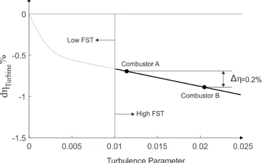
1-1 Change in lost HPT stage efficiency due to combustor turbulence, plot-ted against combustor turbulence level in terms of the TLR parameter, defined in Chapter 2. Designs A and B represent two engine-realistic combustor design configurations that are described in Chapter 8. This figure demonstrates an outcome of this work, namely, a relationship be-tween HPT performance and combustor turbulence parameters, that can be related to combustor design parameters. . . 32

2-1 Fractional increase in 𝑐𝑓 from a range of data sources. The solid blue

line in (a) represents the curve-fit proposed by Stefes [49] and in (b) represents a line of best-fit based on the data considered in this study. The ‘other measurements’ in (a) refer to skin-friction measurements from Hancock & Bradshaw [26], Thole & Bogard [51], Bott & Bradshaw [8] considered by Stefes [49] in the determination of his curve-fit. The shaded region represents uncertainty due to the scatter in 𝑐𝑓 data. . . 42

2-2 Relationship between the FST dissipation length-scale, intensity and the TLR turbulence parameter. This figure shows that the lower asymptote of our definition of high-FST is TLR = 0.01. . . 44

2-3 Skin-friction measurements in the presence of FST from a range of data sources. The solid line represents Esteban’s curve-fit for low-FST [20]. The shaded region represents a 5% uncertainty above and below the respective curve fit to account for the typical magnitude of uncertainty in 𝑐𝑓 measurements [17, 20, 22, 48]. . . 47

(14)

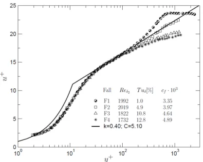
3-1 Inner-normalized mean velocity profiles of a zero-pressure gradient tur-bulent boundary layer for different turbulence intensities, 𝑇 𝑢𝛿99.5 =

1.0% − 12.8% and 1700 . 𝑅𝑒𝜃 . 2000 (Stefes and Fernholz [48]). The

solid line represents the log-law with coefficients 𝜅 = 0.40 and 𝐴 = 5.10. 62

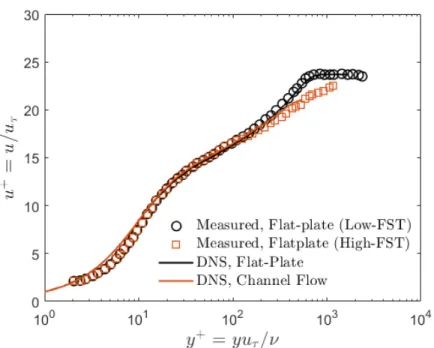
3-2 Inner-normalized mean velocity profiles for a zero-pressure gradient turbulent boundary layer over a range of turbulence intensities (𝑇 𝑢𝛿99.5 =

0.6% − 12.7%) for 2800 . 𝑅𝑒𝜃 . 5600 (Dogan [17]). The dashed line

represents the log-law with coefficients 𝜅 = 0.3884 and 𝐴 = 4.4. The solid line represents DNS channel flow computations at 𝑅𝑒𝜏 = 2000

[31]. The inset shows a close-up of the profiles for the range of 600 < 𝑦+ _{< 1500.} _{. . . .} ₆₂

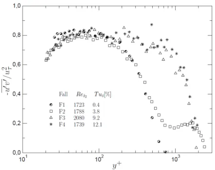
3-3 Measured inner-normalized Reynolds shear stress profiles of a zero-pressure gradient turbulent boundary layer for a range of turbulence intensities (𝑇 𝑢𝛿99.5 = 1.0% − 12.8%); 1700 . 𝑅𝑒𝜃 . 2000 (Stefes and

Fernholz [48]). . . 64

3-4 Measured inner-normalized Reynolds shear stress profiles of a zero-pressure gradient turbulent boundary layer for a range of turbulence intensities (𝑇 𝑢𝛿99.5 = 7.4%, 12.7%); 2800 . 𝑅𝑒𝜃 . 5600 (Dogan [17]).

The solid line represents DNS channel flow data at 𝑅𝑒𝜏 = 4200 [36]. . 64

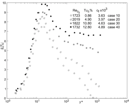
3-5 Profiles for Reynolds normal stress, Ę(𝑢′₎2+ _{in inner-scaling of a}

zero-pressure gradient turbulent boundary layer measured for a range of turbulence intensities (𝑇 𝑢𝛿 99.5 = 0.4% − 12.8%) for 1700 . 𝑅𝑒𝜃 . 2000

(15)

3-6 (i) Contour maps of the inner-normalized pre-multiplied energy spec-tra of the streamwise velocity fluctuations, 𝑘𝑥𝜑𝑢𝑢/𝑢2𝜏, for cases (a)

𝑇 𝑢 = 7.4%; (b) 𝑇 𝑢 = 8.3%; (c) 𝑇 𝑢 = 12.1%; (d) 𝑇 𝑢 = 12.7%. The or-dinates show streamwise wavelength, 𝜁𝑥, in both inner (left) and outer

(right) scaling. The abscissas show the wall normal location, 𝑦, also plotted in both inner (bottom) and outer (top) scaling. (+) indicates inner (black) and outer (white) spectral peaks [17]. (ii) Dogan’s corre-sponding mean (blue outlined marker) and variance profiles. Dashed red line: log-law with coefficients 𝜅 = 0.384 and 𝐴 = 4.4. Dot-dashed vertical lines and (+) symbols represent the locations corresponding to the spectral peaks indicated on (i) [17]. . . 67

3-7 Dogan’s variance profiles of scale-decomposed streamwise velocity fluc-tuations [17]. (a) Small scales and (b) large scales based on a cut-off wavelength filter of 𝜁+

𝑥 = 4000, which corresponds to 𝜁𝑥/𝛿 ≈ 1−2 for all

cases; filled triangle case: 𝑇 𝑢 = 7.4%, 𝑅𝑒𝜃 = 2760; filled diamond case:

𝑇 𝑢 = 8.3%, 𝑅𝑒𝜃 = 4870; filled right triangle case: 𝑇 𝑢 = 12.1%, 𝑅𝑒𝜃 =

4360; and filled square case: 𝑇 𝑢 = 12.7%, 𝑅𝑒𝜃 = 5590. . . 68

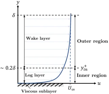
4-1 Schematic of a turbulent boundary layer illustrating the inner-region and the outer-region classification. . . 73

4-2 Contribution of the different sub-components of 𝑐𝐷(as defined in

Equa-tion 4.2) to total 𝑐𝐷, calculated using DNS profiles for flat-plate

turbu-lent boundary layers for a range of 𝑅𝑒𝜃 values [41]. This figure

quanti-fies the contribution of, and hence relative significance of, the various sub-components of 𝑐𝐷 when evaluating the uncertainty associated with

(16)

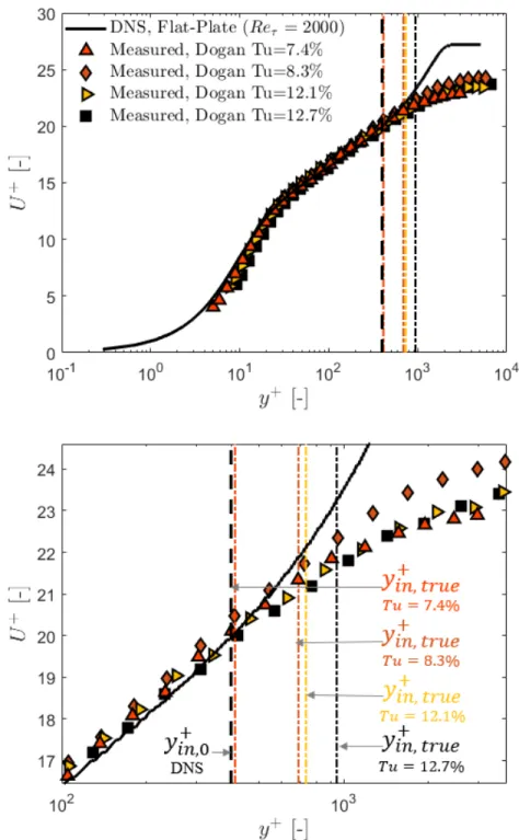
4-3 Inner-normalized mean velocity profiles for a zero-pressure gradient turbulent boundary layer over a range of turbulence intensities (𝑇 𝑢𝛿∞ =

7.4% − 12.7%) for 2800 . 𝑅𝑒𝜃 . 5600 (Dogan [17]). The solid line

represents DNS channel flow computations at 𝑅𝑒𝜏 = 2000 [31]. The

dashed vertical lines represent the limit of the inner-region, the dis-tance up to which the log-law is considered valid, 𝑦_𝑖𝑛+ ≈ 0.2𝑅𝑒𝜏, for the

various cases. The bottom figure shows a close-up of the profiles to indicate how 𝑦_{𝑖𝑛,𝑡𝑟𝑢𝑒}+ in the presence of FST deviates from the defined fixed limit of 𝑦+_𝑖𝑛,0, but is nonetheless always greater than 𝑦_𝑖𝑛,0+ . . . 75

4-4 Effect of suppressed wake in presence of FST on mean velocity gradient can be quantified by comparing flat-plate DNS data (𝑅𝑒𝜏 = 690 or

𝑅𝑒𝜃 = 1970 [46, 33]), which agrees with low-FST measurements [48],

with channel-flow DNS data (𝑅𝑒𝜏 = 540 [35]), which agrees with

high-FST measurements [48]. . . 78

4-5 Inner-normalized profiles for production of TKE, Π+ = −Ě𝑢′_𝑣′+ 𝜕𝑢+ 𝜕𝑦+, of

a zero-pressure gradient turbulent boundary layer measured for a range of turbulence intensities (𝑇 𝑢∞ = 0.4% − 12.1%) for 1700 . 𝑅𝑒𝜃 . 2000

by Stefes and Fernholz [48]. These profiles are used to justify the assumption that Π+ _{profiles can be assumed to be universal in the}

presence of FST. . . 83

4-6 Inner-normalized profiles for Reynolds shear stress, Π+ = −Ě𝑢′_𝑣′+_,

and mean velocity gradient, 𝜕𝑢_𝜕𝑦++, of a zero-pressure gradient

turbu-lent boundary layer. The colored data points represent the measured Reynolds shear stress for a range of turbulence intensities (𝑇 𝑢∞ =

0.4% − 12.8%) for 1700 . 𝑅𝑒𝜃 . 2000 by Stefes and Fernholz [48]. The

solid black line represents the mean velocity gradient profile and the dashed black line represents the Reynolds shear stress profile from DNS data for a flat-plate at 𝑅𝑒𝜃 = 1970 [33, 46]. These profiles are used to

(17)

4-7 Fractional increase in 𝑐𝐷 calculated as a function of the fractional

in-crease in 𝑐𝑓 using different methods and data sources, as listed in Table

4.1. The shaded band represents a 15% uncertainty in fractional in-crease in 𝑐𝑓 which translates to a 25% − 27% uncertainty in fractional

increase in 𝑐𝐷 using Indirect Method I (Equation 4.22). This figure

quantifies the accuracy of the two indirect methods for total 𝑐𝐷,

rela-tive to results from the direct method. . . 98

4-8 Fractional increase in sub-components of 𝑐𝐷 (based on physical loss

mechanism) calculated as a function of the fractional increase in 𝑐𝑓

using different methods and data sources, as listed in Table 4.1. This figure quantifies the accuracy of the two indirect methods for 𝑐𝐷,𝑚𝑒𝑎𝑛

and 𝑐𝐷,𝑇 𝐾𝐸, relative to results from the direct method. . . 102

4-9 Fractional increase in sub-components of 𝑐𝐷,𝑇 𝐾𝐸 (based on location of

loss generation) calculated as a function of the fractional increase in 𝑐𝑓

using different methods and data sources, as listed in Table 4.1. This figure quantifies the accuracy of the Indirect Method I for 𝑐𝐷,𝑇 𝐾𝐸,𝑖𝑛𝑛𝑒𝑟

and 𝑐𝐷,𝑇 𝐾𝐸,𝑜𝑢𝑡𝑒𝑟, relative to results from the direct method. . . 103

5-1 Velocity-defect profiles measured by Stefes et. al [48] in outer-law scaling for various FST levels. The solid line is the log-law profile: 𝑢+_{= (1/𝜅)𝑙𝑛𝑦}+_{+ 𝐶, where 𝜅 = 0.40 and 𝐶 = 5.10, and represents the}

baseline no/low-FST case. This figure demonstrates the deviation of velocity-defect profiles in FST from the baseline no/low-FST case. . . 109

5-2 Velocity-defect ( ¯𝑢𝑒− ¯𝑢)/𝑢𝜏 versus 𝑦/𝛿99.5 in no or low-FST from DNS

[41] for different streamwise locations. The figure demonstrates that velocity-defect profiles collapse in the wake-region. . . 109

(18)

5-3 Velocity-defect ( ¯𝑢𝑒− ¯𝑢)/𝑢𝜏 versus 𝑦/𝛿99.5 in combustor turbulence [22]

for different streamwise locations. The figure demonstrates the de-viation of velocity-defect profiles, greater than the 4.5% uncertainty expected for the velocity-defect measurements (indicated by shaded bands along velocity-defect profiles), in the wake-region, with FST. . 110

5-4 Integrated rate of advection of TKE, computed using Folk’s hot-wire measurements [22] in the presence of grid (low) turbulence and com-bustor (high) turbulence, and normalized using inner-units, plotted against 𝑅𝑒𝜃. This figure shows that the low-FST advection

measure-ments (representing the left-hand side of Equation 5.6, indicated by orange markers) fall within the 5% uncertainty range (set by the right-hand side of Equation 5.6, indicated by orange shaded region), thus providing evidence that a low-FST flat-plate BL can be considered to be in equilibrium. On the other hand, high-FST measurements do not satisfy Equation 5.6, and are hence, not in equilibrium. . . 113

5-5 Sketch representing control volume over which Equation 5.4 is inte-grated. Since the control volume has a single inlet and exit, and is bounded by a mean streamline on top, mass flux entering from the left side of the control volume is equal to the mass flux leaving from the right side of the control volume. The top of the control volume lies in the freestream where production of TKE is negligible. The turbulence stresses are non-zero along this streamline . . . 114

5-6 Integrated production (∫︀₀𝑦+Π𝑑𝑦+), advection (∫︀₀𝑦+[𝜕/𝜕𝑥(𝑢𝑞2_)]𝑑𝑦+_{), and}

dissipation (∫︀₀𝑦+𝜖𝑑𝑦+_{) terms of Equation 5.7, normalized using}

inner-units and plotted against the inner-normalized wall-normal distance. The profiles are obtained from high-FST measurements by Stefes [50] and Folk [22], as well as flat-plate DNS data [46, 33] for 𝑅𝑒𝜃 ∼ 2000.

The figure demonstrates that the integrated contribution of rate of advection to rate of production is not negligible. . . 116

(19)

5-7 Increase in 𝑐𝐷,𝑇 𝐾𝐸 calculated using different methods and data sources,

as listed in Table 4.1, plotted against 𝑇 𝑢3_∞/(𝐿𝑢

𝑒,∞/𝛿99.5). This figure is

used to show that Δ𝑐𝐷,𝑇 𝐾𝐸 does not scale with the function derived in

Equation 5.10.. . . 123

5-8 Increase in 𝑐𝐷,𝑇 𝐾𝐸 calculated using different methods and data sources,

as listed in Table 4.1, plotted against Δ ˜𝐹3 ∝

b 𝑇 𝑢5

∞𝑅𝑒𝜃(𝐿𝑢𝑒,∞/𝜃)(𝑐𝑓/2).

This figure is used to show that Δ𝑐𝐷,𝑇 𝐾𝐸 does not scale with the Δ ˜𝐹3

alone; the contribution of (Δ ˜𝐸∞+ Δ ˜𝑄𝐿𝑆) to Δ𝑐𝐷,𝑇 𝐾𝐸 (in Equation

5.11) cannot be neglected. . . 124

6-1 Relationship between the scaling-parameter, 𝜆, and (a) 𝑇 𝑢∞ for

se-lected values of 𝐿𝑢

𝑒,∞/𝛿, and (b) 𝐿𝑢𝑒,∞/𝛿 for selected values of 𝑇 𝑢∞,

computed using Equation 6.25. This figure demonstrates that 𝜆 de-creases below 1 (i.e. deviation from equilibrium) as 𝑇 𝑢∞increases and

𝐿𝑢_𝑒,∞/𝛿 decreases. . . 139

6-2 Relationship between the outer-region shear stress coefficient in non-equilibrium conditions and (a) 𝑇 𝑢∞ for selected values of 𝐿𝑢_𝑒,∞/𝛿, and

(b) 𝐿𝑢_𝑒,∞/𝛿 for selected values of 𝑇 𝑢∞, computed using Equations 6.25

and 6.26. . . 141

7-1 Estimated relationship between fractional increase in 𝑐𝐷, calculated

using different methods and data sources, as listed in Tables 4.1 and 7.1, and (a) empirical FST parameter, HBB, and (b) analytical FST parameter, TLR. . . 146

7-2 Fractional increase in sub-components of 𝑐𝐷 (based on physical loss

mechanism) calculated using different methods and data sources, as listed in Tables 4.1 and 7.1, plotted against the TLR parameter. . . . 147

7-3 Fractional increase in sub-components of 𝑐𝐷 (based on location of loss

generation) calculated using different methods and data sources, as listed in Tables 4.1 and 7.1, plotted against the TLR parameter. . . . 149

(20)

7-4 Fractional increase in 𝑐𝐷,𝑇 𝐾𝐸,𝑜𝑢𝑡𝑒𝑟 calculated using different methods

and data sources, as listed in Tables 4.1 and 7.1, plotted against the HBB and TLR parameters. . . 150

7-5 Estimated relationship between the fractional increase in 𝑐𝐷,𝑜𝑢𝑡𝑒𝑟,

cal-culated in equilibrium conditions using Equation 7.1a, and in non-equilibrium conditions calculated using Equation 7.2, and empirical FST parameter, TLR, for (a) selected 𝑇 𝑢∞ cases, and (b) selected

𝐿𝑢_𝑒,∞/𝛿 cases. . . 151

7-6 Estimated relationship between fractional increase in 𝑐𝐷, calculated

in equilibrium conditions using Equation 7.1a and in non-equilibrium conditions using Equation 7.2, and empirical FST parameter, TLR, for (a) selected 𝑇 𝑢∞ cases, and (b) selected 𝐿𝑢_𝑒,∞/𝛿 cases. . . 153

7-7 Fractional increase in (a) 𝑐𝐷,𝑚𝑒𝑎𝑛 and (b) 𝑐𝐷,𝑖𝑛𝑛𝑒𝑟 calculated using

dif-ferent methods and data sources, as listed in Tables 4.1 and 7.1, plotted against the TLR parameter. These figures demonstrate the validity of the derived analytical relationship between 𝑐𝐷,𝑚𝑒𝑎𝑛 and 𝑐𝐷,𝑖𝑛𝑛𝑒𝑟 and

TLR (Equation 7.1a).. . . 154

8-1 Agreement between measured and estimated values for the profile stag-nation pressure loss coefficient, 𝑌𝑝, in the presence of combustor

tur-bulence for the baseline case from Folk et al. [23]. . . 160

8-2 Change in stator profile loss due to combustor turbulence. As jet size increases, profile loss of the turbine stator decreases. Baseline is taken from Folk et al. [23], as described in Section 8.1. . . 163

8-3 Change in lost stage efficiency due to combustor turbulence. As jet size increases, efficiency of the turbine stage improves. . . 163

8-4 Change in stator profile loss due to combustor turbulence. As combus-tor length increases, profile loss of the turbine stacombus-tor decreases. . . 164

8-5 Change in lost stage efficiency due to combustor turbulence. As com-bustor length increases, the efficiency of the turbine stage improves. . 165

(21)

B-1 Suction-surface blade-loading distribution for (i) the original loading for the Harrison cascade (𝐴 = 0), and (ii) the quasi-steady model with sinusoidal variations of 𝐴 = 0.10 and 𝜆/𝑐𝑥 = 0.1785, as defined

in Equation B.1. These loading distributions are used as inputs in Equation 3.7 to generate case (3) Figure B-2.. . . 181

B-2 Loss-coefficient, 𝑌𝑝, calculated using Equation 3.7 and the Harrison

blaloading distribution from Figure B-1, for the three cases de-scribed above. The circular markers represent 𝑌𝑝 measurements by

Folk et. al [23] in the presence of grid turbulence (𝑇 𝑢∞ = 1.3%, blue

markers) and combustor turbulence (𝑇 𝑢∞ = 10%, red markers). This

figure demonstrates that the quasi-steady model cannot be used to capture the effect of FST on the loss-coefficient, and that one must account for the change in 𝑐𝐷. . . 182

C-1 Local production (Π), advection (𝑑/𝑑𝑥(𝑢𝑞2_{)), and dissipation (𝜖) terms}

of Equation 5.4, normalized using inner-units and plotted against the inner-normalized wall-normal distance. The profiles are obtained from high-FST measurements by Stefes [50] and Folk [22], as well as flat-plate DNS data [46, 33] for 𝑅𝑒𝜃 ∼ 2000. The figure demonstrates

that the local contribution of rate of advection to rate of production is negligible. . . 184

(22)

(23)

List of Tables

3.1 Experimental results showing the range of turbulence intensities and Reynolds numbers, and the definition of the inner-region within which mean velocity and Reynolds shear stress profiles were found to collapse. 61

4.1 Summary of input data and calculation method used to generate results for fractional rise in 𝑐𝐷, as plotted in Figures 4-7 - 4-9. . . 99

7.1 Summary of input data and calculation methods, in addition to those listed previously in Table 4.1, used to generate results for fractional rise in 𝑐𝐷, as plotted in Figures 7-1 - 7-7, against HBB and TLR respectively.145

8.1 Reduction in profile loss, and consequent increase in HPT stage effi-ciency for different combustor design changes (i.e. increasing combus-tor port diameter, lengthening combuscombus-tor and rearranging/re-orienting combustor jets). . . 167

(24)

(25)

Nomenclature

Acronyms

(T)BL (Turbulent) Boundary layer

DNS Direct Numerical Simulation

FST Freestream Turbulence

HBB Hancock, Bradshaw, & Blair Parameter [5]

HPT High-Pressure Turbine

NGV Nozzle Guide Vane

TKE Turbulent Kinetic Energy, per unit mass

TLR Turbulence intensity - Length scale - Reynolds number parameter, as defined by Ames [1]

ZPG Zero-Pressure Gradient

Subscripts

0 Reference value, i.e. when the boundary layer is subjected to no or low FST, as defined in Chapter2

∞ Located in freestream, i.e. where 𝑦 = 𝛿99.5

𝑒𝑞 Evaluated for boundary layer in equilibrium conditions

(26)

𝑡 Total or stagnation flow quantity

𝑤 Evaluated at the wall

Greek Letters

𝛼2 Exit flow angle

𝛿 Boundary layer thickness

𝛿* Displacement thickness, ∫︀₀𝑦∞p1 − 𝑢/𝑈∞q 𝑑𝑦 𝛿𝑒 Energy-loss thickness, ∫︀𝑦∞ 0 p𝑢/𝑈∞q r1 − (𝑢/𝑈∞) 2 s 𝑑𝑦 𝛿𝑠 Entropy thickness, 𝛿𝑠= _𝜌𝑈𝑇∞3 ∞ ∫︀𝑦∞ 0 p𝜌𝑢Δ𝑠q 𝑑𝑦

𝛿99.5 Boundary layer thickness, 𝛿99.5 = 𝑦(𝑢/𝑈∞= 0.995)

Δ𝐸𝑄 Deviation from equilibrium of turbulent boundary layer

𝜖 Rate of viscous dissipation of turbulent kinetic energy

𝜂𝑠𝑡𝑎𝑔𝑒 HPT stage efficiency

𝜆 Lag constant scaling parameter

Λ𝑢𝑢 Integral length scale (streamwise direction)

𝜇 Dynamic viscosity of the fluid

𝜈 Kinematic viscosity of the fluid

𝜑 Rate of viscous dissipation of mean kinetic energy

Π Rate of production of turbulent kinetic energy

𝜌 Density of the fluid

(27)

𝜏 Total shear-stress in the 𝑥𝑦-plane, 𝜌`𝜈𝜕𝑢/𝜕𝑦 − 𝑢′_𝑣′˘

; In Chapter 6, 𝜏 = −𝜌𝑢′_𝑣′

𝜏𝑤 Shear-stress at the wall

𝜃 Momentum-loss thickness, ∫︀₀𝑦∞p𝑢/𝑈∞q p1 − 𝑢/𝑈∞q 𝑑𝑦

𝜉 Entropy loss coefficient, 𝜉 = 𝛿𝑠

𝜎𝑐𝑜𝑠(𝛼2)𝑐

3/2 𝑝

𝑑𝜂𝑠𝑡𝑎𝑔𝑒 Change in lost HPT stage efficiency due to combustor turbulence effects

Superscripts

+ Indicates inner-scaling, also referred to inner-normalization. The vari-ables are non-dimensionalized using 𝑢𝜏 and 𝜈

¯

( ) Time-averaged quantity

˜

( ) Modified variable that accounts for FST effects

Latin Letters

¯

𝑞2 _{Turbulent kinetic energy, ¯}_𝑞2 _{= (𝑢}′₎2_{+ (𝑣}′₎2_{+ (𝑤}′₎2

9

𝑆𝑎 Rate of entropy generation per unit surface area

𝑢′_𝑣′ _{Time mean value of product of fluctuation components 𝑢}′ _{and 𝑣}′ _acting vertically to one another; −𝜌𝑢′_𝑣′ _{is also denoted as Reynolds shear} stress

𝑎1 Ratio of turbulent shear stress to TKE, 𝑎1 = 𝜏 /𝜌 ¯𝑞2

𝑐𝜏 Shear-stress coefficient

𝑐𝐷 Dissipation coefficient

𝑐𝑓 Local skin-friction coefficient, 2(𝑢𝜏/𝑈∞)2

(28)

𝑐𝑥 Axial blade chord

𝑐𝜏,𝑒𝑞 Shear-stress coefficient for equilibrium BL

𝑐𝐷,𝑖𝑛𝑛𝑒𝑟 Sub-component of 𝑐𝐷 from the inner-region of the boundary layer

𝑐𝐷,𝑙𝑎𝑚 Dissipation coefficient in laminar flow

𝑐𝐷,𝑚𝑒𝑎𝑛,𝑖𝑛𝑛𝑒𝑟 Sub-component of 𝑐𝐷,𝑚𝑒𝑎𝑛 from the inner-region of the boundary layer

𝑐𝐷,𝑚𝑒𝑎𝑛,𝑜𝑢𝑡𝑒𝑟 Sub-component of 𝑐𝐷,𝑚𝑒𝑎𝑛 from the outer-region of the boundary layer

𝑐𝐷,𝑚𝑒𝑎𝑛 Component of 𝑐𝐷 due to viscous dissipation of mean kinetic energy

𝑐𝐷,𝑜𝑢𝑡𝑒𝑟 Sub-component of 𝑐𝐷 from the outer-region of the boundary layer

𝑐𝐷,𝑇 𝐾𝐸,𝑖𝑛𝑛𝑒𝑟 Sub-component of 𝑐𝐷,𝑇 𝐾𝐸 from the inner-region of the boundary layer

𝑐𝐷,𝑇 𝐾𝐸,𝑜𝑢𝑡𝑒𝑟 Sub-component of 𝑐𝐷,𝑇 𝐾𝐸 from the outer-region of the boundary layer

𝑐𝐷,𝑇 𝐾𝐸 Sub-component of 𝑐𝐷 due to production of turbulent kinetic energy

𝐷𝑝𝑜𝑟𝑡 Combustor port diameter

𝑒 Relative fluctuating strain rate

𝐺 Non-dimensional parameter relating rate of diffusion of TKE to local shear-stress, 𝐺 ≡ ´ Ě 𝑝′_𝑣′ 𝜌 + 1 2𝑞Ě2𝑣 ′¯_/´𝜏𝑚𝑎𝑥 𝜌 ¯1/2 𝜏 𝜌

𝐻12 Shape factor (or form parameter), 𝛿*/𝜃

𝐻32 Energy shape factor, 𝛿𝑒/𝜃

𝐾𝑐 Lag constant, 𝐾𝑐= 2𝑎_𝑢𝐿1𝑈∞_𝜏 𝛿

𝐿𝜏 Shear-stress based length-scale, 𝐿𝜏 = (𝜏 /𝜌)3/2/𝜖

𝐿𝑐 Combustor length

(29)

𝑙𝑚 Mixing length-scale (characteristic length of large turbulence elements), 𝑙𝑚 = 𝜅𝑦 for 𝑦/𝛿 < 0.2; 𝜅 ∼ 0.4

𝑝 Mean (i.e. time-averaged) value of static pressure

𝑝′ Fluctuating component of static pressure

𝑅𝑒𝜏 Reynolds number based on skin-friction velocity, 𝑢𝜏𝛿99.5/𝜈

𝑅𝑒𝜃 Reynolds number based on momentum thickness, 𝑈∞𝜃/𝜈

𝑆′ Strain rate tensor

𝑇 Mean (i.e. time-averaged) value of static temperature

𝑡 Time

𝑇 𝑢 Turbulence Intensity (streamwise direction)

𝑢′, 𝑣′, 𝑤′ Components of the turbulent fluctuation velocities in the streamwise (𝑥), transverse (𝑦), and spanwise (𝑧) directions

𝑢, 𝑣, 𝑤 Mean (i.e. time-averaged) velocity component in the streamwise (𝑥), transverse (𝑦), and spanwise (𝑧) directions

𝑈∞ Mean (i.e. time-averaged) freestream velocity in the streamwise (𝑥) direction

𝑢𝜏 Skin-friction velocity, a

𝜏𝑤/𝜌

𝑥, 𝑦, 𝑧 Coordinates (𝑥, 𝑧 parallel to the wall; 𝑦 perpendicular distance from the wall

(30)

(31)

Chapter 1 Introduction

1.1 Motivation

In a gas turbine engine, the role of the combustor is to combine fuel and air efficiently. One of the ways the combustor does this is through turbulent mixing, created for example by impinging jets in cross-flow. The turbulence generated by the mixing process convects downstream to the high-pressure turbine (HPT). To optimize the performance of both of these components we should not consider their designs sep-arately; HPT performance depends on combustor turbulence and combustor design can change the level, size, and shape of turbulence.

A potential benefit in the trade-off between combustor design and HPT perfor-mance is shown in Figure 1-1, taken from the current study. The plot shows that turbine efficiency, calculated for a hypothetical HPT stage, is a function of inlet tur-bulence. The horizontal axis represents the level, size, and shape of turtur-bulence. The details of this plot will be explained later in this thesis but the key take away is that a feasible change in combustor geometry from Design A to Design B can have a +0.2% improvement in turbine stage efficiency.

Figure1-1also shows two regimes of freestream turbulence (FST) on the horizontal axis. On the left-hand side is the low-FST regime and on the right is the high-FST regime. Chapter2quantifies and explains the turbulence parameter and this threshold in detail. For now it is important only to highlight that this study will focus on the

(32)

high-FST regime. This regime most accurately represents the combustor-turbine interface in a gas turbine engine.

Figure 1-1: Change in lost HPT stage efficiency due to combustor turbulence, plot-ted against combustor turbulence level in terms of the TLR parameter, defined in Chapter 2. Designs A and B represent two engine-realistic combustor design configu-rations that are described in Chapter 8. This figure demonstrates an outcome of this work, namely, a relationship between HPT performance and combustor turbulence parameters, that can be related to combustor design parameters.

1.2 Research Objective

The objective of this study is to relate key freestream turbulence parameters, i.e. tur-bulence intensity and dissipation length-scale, to the dissipation coefficient, a measure of loss generation in boundary layers. Doing this can provide guidelines to optimize the trade between combustor turbulence and turbine aerodynamic performance.

1.3 Thesis Contributions

1. A major contribution of this study is a derived relationship between HPT stage efficiency and combustor turbulence parameters, as shown qualitatively in Fig-ure 1-1.

(33)

2. We also define regimes of the freestream turbulence impact on turbulent bound-ary layers, drawing a distinction between low-FST, which has negligible effect on boundary layer loss generation, and high-FST, which has measurable effect on boundary layer loss generation.

3. We enable the establishment of design trade-offs and optimization of perfor-mance between the combustor and HPT by quantifying the relationship between combustor design parameters and HPT performance.

4. We provide insight into the uncertainty associated with HPT stage efficiency calculations due to effects of combustor turbulence.

5. We give specific guidelines to account for the effects of freestream turbulence in computational procedures through the fundamental relationship between boundary layer loss generation and freestream turbulence parameters.

1.4 Thesis Chapter Organization

In Chapter2, we define freestream turbulence (FST) and identify the key FST param-eters needed to quantify the impact of FST on loss generation in turbulent boundary layers (TBLs). This includes characteristic FST metrics to quantify the level of FST and establish a distinction between low and high-FST conditions. Chapter 3 gives findings from literature regarding the effect of high-FST on the skin-friction coef-ficient, 𝑐𝑓, as well as other TBL parameters. We also justify the selection of the dissipation coefficient, 𝑐𝐷, as the metric for loss generation. We derive a link between skin-friction and dissipation coefficients in Chapter4with the objective of converting the measured response of boundary layers to high-FST in terms of 𝑐𝑓, to the loss met-ric 𝑐𝐷. In Chapter 5, we show evidence for and explain the importance of accounting for non-equilibrium behavior of the TBL in the presence of FST and then propose a method to account for non-equilibrium effects on 𝑐𝐷 in Chapter 6. The results of the methods derived in Chapters4and6are described in Chapter7. The results are used in example trade-studies, in Chapter8, between HPT stage efficiency and combustor

(34)

design parameters, which demonstrate application of the methodology. Chapter 9

(35)

Chapter 2 Definition of Freestream Turbulence

Levels

In this chapter, we define freestream turbulence and distinguish between low and high freestream turbulence.

2.1 Definition of Freestream Turbulence (FST)

2.1.1 Assumptions Regarding Freestream in Presence of FST

The freestream in this study is defined as the region in a wall-bounded flow be-yond which the time-averaged quantities and turbulence intensities cease to vary in wall-normal direction, 𝑦.1 _{The conceptual boundary between the freestream and the}

boundary layer is useful in distinguishing between turbulence eddies produced in the boundary layer and those produced by the external source of freestream turbulence, such as a grid or jets in cross-flow.

2.1.2 Characterization of FST

Turbulence is characterized using a number of parameters:

1_{Uniform turbulence in the 𝑦−direction implies negligible diffusion of turbulent kinetic energy,} and absence of mean-velocity gradient in the 𝑦−direction implies negligible production of turbulent kinetic energy for a two-dimensional flow.

(36)

1. Turbulence intensity: the magnitude of velocity fluctuations relative to the time-averaged freestream velocity, and hence, the average amount of turbulent kinetic energy contained in the largest eddies;

2. Length-scales: the size and turn-over rate of various eddies; defined and mea-sured differently based on the application;

3. Extent of anisotropy: a measure of the shape of the eddies (e.g. isotropic turbulence consists of spherical eddies);

4. Reynolds shear stress: a measure of the extent of symmetry of various eddies, responsible for the transfer of momentum;

5. Reduced frequency: a measure of the time-scales associated with turbulent fluctuations, relative to the time-scales associated with propagation of changes in the bulk flow.

For this study, we have selected freestream turbulence intensity, and the ratio of a characteristic freestream turbulence length-scale to a characteristic boundary layer length-scale as the two key parameters necessary to determine the effect of freestream turbulence on turbulent boundary layers (TBLs). Additionally, we consider the effect of a non-zero Reynolds shear stress in the freestream on loss-generation in TBLs under the influence of FST.

Turbulence Intensity

The turbulence intensity quantifies the magnitude of streamwise velocity fluctuations, 𝑢′, relative to the time-averaged freestream velocity, 𝑈∞, in Equation 2.1.

𝑇 𝑢∞ = a (𝑢′₎2 ∞ 𝑈∞ (2.1)

FST with higher levels of 𝑇 𝑢∞ has a greater influence on the outer-layer mixing of the boundary layer, resulting in larger near-wall gradients, a fuller velocity profile, and smaller outer-layer gradients [1].

(37)

Ratio of Characteristic FST Scale to Characteristic BL Length-Scale

The effect of FST on TBLs depends not only on the turbulence intensity level but also on the size of turbulence. We have selected the dissipation length scale as the characteristic length-scale for FST. The rationale for selecting the dissipation length scale is discussed below.

Dissipation Length Scale as Characteristic FST Length Scale:

The turbulence length scale typically reported in literature is the longitudinal integral length scale, Λ𝑢𝑢, which represents the size of large coherent structures in the stream-wise direction of the flow, i.e. of 𝑢′ fluctuations. Turbulence is also characterized in terms of a dissipation length scale, 𝐿𝑢_𝑒. This length scale physically represents the turn-over rate of large eddies, which in turn dictates the rate of decay of turbulent kinetic energy. The ratio 𝐿𝑢_𝑒/Λ𝑢𝑢is typically order of magnitude of one [5,47,51], and 𝐿𝑢

𝑒 and Λ𝑢𝑢 can be (and have been) used interchangeably. However, measurements of freestream turbulence from combustor simulators indicate that 𝐿𝑢_𝑒/Λ𝑢𝑢 > 𝑂(1) [1, 22]. Therefore, the size of an eddy in terms of the longitudinal extent of veloc-ity fluctuations and the size of an eddy in terms of the rate at which the eddy is able to pass down energy to smaller eddies are different in the presence of freestream turbulence.2

In Chapter 5, we show that loss generation in a TBL is a function of the rate of advection of freestream turbulence, and hence, the rate of dissipation of freestream turbulence. We therefore select the dissipation length scale as the characteristic length-scale of freestream turbulence. This choice of length-scale is in agreement with studies on the effect of FST on 𝑐𝑓 and heat-transfer in TBLs [1, 26].

For isotropic turbulence, the dissipation length-scale is defined in Equation 2.2

2_{The observation that the length scale associated with energy dissipation is greater than the} length scale associated with the size of an eddy is in agreement with Ames’s streamwise turbulence decay measurements [1] which show that turbulence generated using a combustor simulator, relative to grid turbulence, decays at a slower rate in the streamwise direction. Therefore, we can conclude that the rate of dissipation of energy in an eddy is lower than the amount of energy contained in the eddy in large-scale freestream turbulence generated using combustor simulators.

(38)

where 𝜖 is the dissipation rate of FST [47].

𝐿𝑢_𝑒 = 3 2

(𝑢′₎23/2

𝜖 (2.2)

Since we have assumed that the production and diffusion of turbulent kinetic energy in the freestream are negligible, the streamwise change in turbulence level can be related to the dissipation rate in the freestream using the dissipation length scale, as in Equation 2.3. − 𝑈∞ 𝑑(𝑢′₎2 𝑑𝑥 = 2 3𝜖 = (𝑢′₎23/2 𝐿𝑢 𝑒 (2.3)

Recent studies involving spectral analysis of the interaction between freestream eddies and boundary layer eddies [17, 44] characterize the effect of FST in terms of the length scale of the eddy containing most energy, 𝜁𝑥. This length scale is often referred to as the most energetic length scale but it does not contain information about the rate of decay of turbulence. Additionally, this length-scale can only be calculated from detailed spectral analysis and cannot be compared with data available from most studies. Thus, we do not use it as a metric to quantify the level of FST, although we use results from measurements of such length-scales to derive the relationship between loss generation in boundary layers and 𝐿𝑢_𝑒,∞.

There are other turbulence length scales that represent the rate of dissipation of turbulent kinetic energy, such as the Taylor micro-scale, 𝜆 =

b

15𝜈(𝑢′₎2_{/𝜖, and the} Kolmogorov scale, 𝜂 = (𝜈3/𝜖)1/4. These length scales represent the turn-over rate of the smallest eddies, whereas 𝐿𝑢

𝑒,∞ represents the turn-over rate of the largest eddies. Most of the turbulent kinetic energy is contained in the large eddies, and therefore, the momentum and energy exchange phenomena are dominated by the large eddies. Additionally, since the effects of viscosity in the freestream are small (i.e. the Reynolds number of the turbulence in the freestream is much larger than that in the boundary layer) we can limit our focus to the dissipation length-scale associated with the large eddies. Therefore, we select 𝐿𝑢

𝑒,∞ as the characteristic length-scale for freestream turbulence in this study.

(39)

Characteristic Length-Scale for BL:

We select the boundary layer thickness, 𝛿99.5 (i.e. the height at which the averaged streamwise velocity in the boundary layer is equal to 99.5% of the time-averaged streamwise velocity in the freestream), as the characteristic length-scale for the boundary layer in this study.

Observations from literature indicate that the effect of freestream turbulence on a TBL decreases as the length-scale ratio, 𝐿𝑢_𝑒,∞/𝛿, increases [26]. Traci and Wilcox [53] noted that for small length scale ratios, the rate of dissipation of turbulence in the boundary layer is increased. This is because dissipation of turbulent kinetic energy occurs at the smallest scales where the effects of viscosity are comparable to those of inertial forces associated with the turbulent fluctuations. Furthermore, Traci and Wilcox [53] stated that at larger length scale ratios, the effects of freestream turbulence on the TBL will lessen, and are expected to have little or no effect at very large length scale ratios. Therefore, we expect loss generation to be inversely proportional to the length-scale ratio, and will quantify the level of FST in terms of a metric that decreases as 𝐿𝑢

𝑒,∞/𝛿 increases.

2.1.2.1 Reynolds Shear-Stress

A non-zero Reynolds shear-stress in the freestream indicates that the turbulence ed-dies are not symmetric. This implies that turbulent momentum can be transported across the interface between the freestream and the boundary layer, which can in-fluence the generation of loss in a turbulent boundary layer. However, extensive measurements of the freestream Reynolds shear-stress cannot be found in literature. Hence, we do not include the non-zero freestream Reynolds shear-stress in the quan-titative metric that scales with the level of FST. Nonetheless, we derive a relationship between boundary layer loss generation and a non-zero freestream Reynolds shear-stress in this study. We also quantify the effect of this parameter on loss-generation for the few data points at which freestream Reynolds shear-stress measurements are available, and discuss the physical implications of the result.

(40)

2.1.3 Quantification of Level of FST

Having identified the key parameters needed to determine the effect of FST on TBLs, we select two metrics that can be used to quantify the level of FST.

Hancock-Bradshaw-Blair (HBB) parameter

Hancock and Bradshaw [27] observed that the effect of FST on the structure of a TBL increases with increasing levels of turbulence intensity and that the TBL structure is less affected at higher dissipation length-scales. They concluded that the structure of the TBL is dependent on the fluctuating strain rate, 𝑒, imposed by the freestream [27]. Since the strain rate imposed by the FST scales upon 𝑢′_∞/𝐿𝑢

𝑒,∞ and the strain rate imposed by the mean motion in the boundary layer scales upon 𝑈∞/𝛿, the relative fluctuating strain rate, 𝑒, as well as the effect of FST on the TBL structure is directly proportional to 𝑇 𝑢∞ and inversely proportional to 𝐿𝑢𝑒,∞/𝛿 [27]. Based on measurements for the increase in 𝑐𝑓 at a given 𝑅𝑒𝜃 in the presence of FST, Hancock and Bradshaw [27] devised a FST parameter, 𝛽 = 𝑇 𝑢∞/(𝐿𝑒,∞/𝛿99.5+ 2) [27]. Blair [5] added a damping term to this parameter to account for low Reynolds number effects. This modified−𝛽 parameter is known as the HBB parameter, and is defined in Equation 2.4. 𝐻𝐵𝐵 = 100 · 𝑇 𝑢∞ „ˆ 𝐿𝑢 𝑒 𝛿99.5 + 2 ˙ ´ 1 + 3𝑒−𝑅𝑒𝜃400 ¯−1 (2.4)

In Equation 2.4, 𝑅𝑒𝜃 is a Reynolds number based on the TBL momentum-thickness, 𝜃, and the time-averaged freestream velocity, 𝑈∞.

The HBB parameter is important because it has been used to correlate the effects of FST on 𝑐𝑓, and hence, it can be used in this study to translate the 𝑐𝑓 = 𝑓 (𝐻𝐵𝐵) measurements to the dissipation coefficient, 𝑐𝐷 (selected metric for loss in TBLs).

(41)

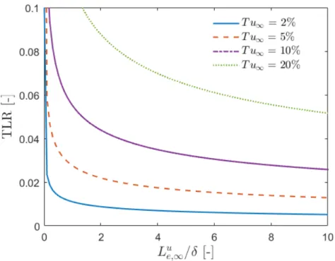
Ames’ Turbulence Intensity - Length-Scale - Reynolds Number (TLR) parameter

Ames [1] suggested using results from rapid distortion theory [32] to analyze the im-pact of large-scale turbulence (relative to the size of the boundary layer) on boundary layers. He noted that freestream perturbations with length-scales that are larger than the size of the boundary layer are less effective in enhancing skin-friction due to the inviscid effect of the wall i.e. attenuation of the normal component of turbulent fluctu-ations for wall-normal distances less than the size of the freestream eddy (𝑦 < 1.3Λ𝑢𝑢, based on Hunt’s calculations [32]). This analysis revealed that the key variables that determine the effect of FST on TBLs were turbulence intensity, Reynolds number, and the length-scale ratio.3 He derived a parameter, commonly referred to as the TLR parameter as defined in Equation 2.5, to correlate the fractional increase in 𝑐𝑓 with FST parameters. 𝑇 𝐿𝑅 = 𝑇 𝑢ˆ 𝜃 𝐿𝑢 𝑒 ˙0.33_{ˆ 𝑅𝑒} 𝜃 1000 ˙0.25 (2.5)

This parameter, derived based on physical relationships between FST and TBL pa-rameters, is used to derive functional relationships between 𝑐𝐷 and FST parameters. Ames’ assumptions in the derivation of TLR [1], and hence, the relationships with TLR derived in this study, are valid for 𝑇 𝑢∞< 0.20 and 𝑅𝑒𝜃𝑇 𝑢∞(𝐿𝑢_𝑒,∞/𝜃) > 4000.

Figures 2-1 (a) and (b) show the fractional increase in 𝑐𝑓 versus HBB and TLR parameters respectively. The shaded band in these figures represents the uncertainty due to the scatter in 𝑐𝑓 data. The curve-fits in the figures are used in following chapters to convert measurements for 𝑐𝑓 = 𝑓 (𝐻𝐵𝐵) and 𝑐𝑓 = 𝑓 (𝑇 𝐿𝑅) to 𝑐𝐷 as a function of HBB and TLR.

Although the boundary layer Reynolds number, 𝑅𝑒𝜃, is used in both Equations

2.4 and 2.5, it does not characterize the FST directly; rather, it is a parameter that can be used to characterize the state of a TBL under the effect of FST. Esteban et al.

3_{Ames’ selected the dissipation length-scale as the characteristic length-scale for FST. However,} he selected the momentum thickness, 𝜃, as the characteristic length-scale for the TBL due to the uncertainty associated with 𝛿 measurements in the presence of FST.

(42)

(a) Fractional increase in 𝑐_𝑓 plotted against the HBB parameter

(b) Fractional increase in 𝑐𝑓 plotted against the TLR parameter

Figure 2-1: Fractional increase in 𝑐𝑓 from a range of data sources. The solid blue line in (a) represents the curve-fit proposed by Stefes [49] and in (b) represents a line of best-fit based on the data considered in this study. The ‘other measurements’ in (a) refer to skin-friction measurements from Hancock & Bradshaw [26], Thole & Bogard [51], Bott & Bradshaw [8] considered by Stefes [49] in the determination of his curve-fit. The shaded region represents uncertainty due to the scatter in 𝑐𝑓 data.

(43)

[20] showed that the trend of 𝑐𝑓 with 𝑅𝑒𝜃 is maintained under the influence of FST. Therefore, the state of the TBL under the influence of FST is expected to vary with 𝑅𝑒𝜃, and the effects of 𝑅𝑒𝜃 need to be accounted for in the characteristic metrics of FST.

2.2 Definition of Low and High-FST

We first define the threshold between the low-FST and high-FST regimes based on the size, level and shape of turbulence. We then define the reference case representing the no or low-FST regime.

2.2.1 Threshold between Low and High-FST

We define the threshold for low and high-FST in terms of the TLR turbulence pa-rameter. Figure 2-2 gives the relationship between the turbulence characteristics (length-scale and intensity) and TLR.

Generally in literature, the level of turbulence is considered high when the turbu-lence intensity is greater than 5% [22]. This is near the maximum level of turbulence intensity that can be generated with conventional static grids [5, 26]. The size of turbulence is considered large when the length-scale is much larger than the size of the downstream boundary layer (e.g. 𝐿𝑢

𝑒,∞/𝛿 > 𝑂(1)).

Figure 2-2 shows that the lower asymptote of our definition of high-FST is TLR= 0.01, which will be the threshold value to discern low and high turbulence in this thesis. This threshold value is consistent with existing measurements of skin-friction on a flat plate in various levels of FST. Figure2-2 shows that for TLR < 0.01, there is very little difference in measured skin-friction from a canonical turbulent boundary layer. For TLR > 0.01 on the other hand, there is a significant rise in skin-friction. This suggests, and our analysis in this thesis will prove, that FST has a negligible effect on the boundary layer when TLR < 0.01, but a significant effect when TLR > 0.01. The aim of this thesis will be to establish the relationship between boundary layer loss and TLR for TLR > 0.01.

(44)

Figure 2-2: Relationship between the FST dissipation length-scale, intensity and the TLR turbulence parameter. This figure shows that the lower asymptote of our definition of high-FST is TLR = 0.01.

Finally, the shape of turbulence is important for quantifying the impact of FST on TBL loss generation. For asymmetric turbulence (i.e. turbulence with non-zero Reynolds shear stress), there is considerably more mixing in the flow compared to symmetric turbulence. Hence, we categorize a turbulence field having a non-zero Reynolds shear stress in the high-FST regime.

2.2.2 Sources of High-FST

This study is motivated by the effects of combustor turbulence on HPT performance. The mechanism that generates turbulence in combustors is opposing jets impinging on each other in the presence of cross-flow. The turbulence intensities at the exit of combustors are typically greater than 10%, and have been found to be as high as 30% as well [4, 10, 12, 43], much different then the grid turbulence of around 1% to 4% used in most turbine cascade and stage testing [22].

(45)

consists of a range of structure sizes, unlike grid turbulence consisting of uniform length-scales set by the grid bar-spacing. The average length-scale of turbulence generated by combustors is set by the size and spacing of the dilution holes, which is much larger than the size of the boundary layer developed on the HPT chord for most real engines [4, 12].

These attributes imply that combustor turbulence falls in the high-FST regime, and that grid turbulence is not appropriate to study the effects of combustor tur-bulence on HPT performance. In order to achieve higher turtur-bulence intensities and obtain a range of eddies of different sizes4, grids with non-uniform geometries or active grids (with moving wings or blowing of high-pressure air) have been used in exper-iments [17, 20]. Studies by Ames [1] and Folk et al. [23] have employed combustor simulators that mix incoming streamwise air and lateral jets in cross-flow, emulating the aerodynamics of a rich-burn combustor. The orientation and relative geomet-ric dimensions of such combustor simulators reflect actual combustor geometry so the turbulence generated reflects actual combustor turbulence characteristics. For instance, Ames [1] reported turbulence intensities as high as 19% at the exit of his combustor simulator test section, and Folk et al. [23] reported intensities as high as 12.6%. Ames [1] and Folk et al. [23] also measured a non-zero Reynolds shear stress in the freestream turbulence. Therefore, measurements from such studies, which result in TLR > 0.01, are referred to as high-FST measurements in this study.

2.2.3 Reference Value for No or Low-FST

2.2.3.1 Reference Value for 𝑐𝑓 in No or Low-FST Conditions

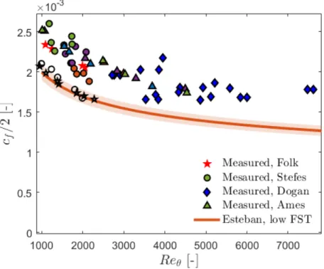
We begin by defining a no or low-FST reference value of the skin-friction coefficient, 𝑐𝑓,0, that can be used to identify and quantify the deviation of 𝑐𝑓 from 𝑐𝑓,0 at a given 𝑅𝑒𝜃 in the presence of FST. In Figure2-3, we evaluated the agreement between skin-friction measurements in FST [1, 17, 22, 48] and Esteban’s low-FST curve-fit [20].

4_{A range of eddies of different sizes is obtained because the flow produced by non-uniform or} active grids generates wakes of sizes that differ in space and time, and consequently interact at different locations downstream of the grid.

(46)

It is clear that this fit is the best choice for correlating 𝑐𝑓,0 values from literature. It is also clear that skin friction measured in high-FST is higher than in low-FST. We thus define low-FST conditions based on Esteban’s low-FST curve-fit [20] for 𝑐𝑓 measurements, as given in Equation2.6,

(2.6) 𝑐𝑓,0= 2 [𝑙𝑜𝑔(𝑅𝑒𝜃)/𝜅 + 𝐶]

−2

where

𝜅 = 0.36 and 𝐶 = 3.193

We use Equation2.6in the following chapters to quantify the rise in 𝑐𝑓, Δ𝑐𝑓 = 𝑐𝑓−𝑐𝑓,0, and hence, the rise in the dissipation coefficient in the presence of FST.

Furthermore, we classify any measurements for 𝑐𝑓 that are more than 5% greater than the value estimated using the curve-fit in Equation 2.6 (i.e. Δ𝑐𝑓/𝑐𝑓,0 > 5%) as being under the influence of high-FST, as shown in Figure 2-3. The acceptable error range of 5% (denoted by shaded band in Figure2-3) was selected based on the average uncertainty associated with 𝑐𝑓 measurements [20].

2.2.3.2 Reference Values for Other TBL Parameters, in No or Low-FST Conditions

For the purposes of this study, we define a TBL to be in no or low-FST if the time-averaged quantities and turbulence statistics of the BL agree, within the measurement uncertainty range, with values from DNS calculations (e.g. in Schlatter and Örlü [42]) having a low freestream turbulence intensity (𝑇 𝑢 = 0.1% at 𝑦 = 2𝛿).5 _{We attribute}

any deviation of the TBL structure in the presence of FST from such DNS calculations to high-FST effects.

5_{We found that such DNS calculations agree with no or low-FST measurements that correspond} to experiments conducted either in the absence of grids or by using passive grids either stationary bar grids, such as in Folk et al.’s experiments [23], or by leaving an active grid installed but with the wings statically located parallel to the flow, such as in Esteban et al. [20] and Dogan et al.’s experiments [17].

(47)

Figure 2-3: Skin-friction measurements in the presence of FST from a range of data sources. The solid line represents Esteban’s curve-fit for low-FST [20]. The shaded region represents a 5% uncertainty above and below the respective curve fit to account for the typical magnitude of uncertainty in 𝑐𝑓 measurements [17, 20, 22, 48].

2.3 Summary

The freestream turbulence intensity, 𝑇 𝑢∞, and dissipation length-scale ratio, 𝐿𝑢_𝑒,∞/𝛿 are the two key parameters characterizing the interaction between FST and TBLs. The HBB and TLR parameters, functions of both 𝑇 𝑢∞and 𝐿𝑢_𝑒,∞/𝛿, have been selected to quantify the level of FST. We classify FST with TLR> 0.01 and/or a non-zero Reynolds shear stress as high-FST.

(48)

(49)

Chapter 3 Characterization of Boundary Layer

Response to FST

This chapter motivates the need for determining the effect of FST on 𝑐𝐷 for flat-plate turbulent boundary layers, and relating 𝑐𝐷 in terms of the widely available skin-friction coefficient, 𝑐𝑓. This chapter also establishes the limit of current knowl-edge regarding boundary layer response to FST. Based on this review, three research questions are presented which will be answered in this thesis.

3.1 Measure of Boundary Layer (BL) Loss

Genera-tion

3.1.1 Definition of the Dissipation Coefficient, 𝑐

𝐷

For turbomachinery, Denton defines loss as ‘any flow feature that reduces the efficiency of a turbomachine’ [15]. Therefore, he recommends quantifying loss in turbomachines in terms of the entropy generation rate, which can be related to the loss in efficiency of a turbomachinery component. Denton [15] converts the entropy generation rate into a dimensionless dissipation coefficient, 𝑐𝐷, defined in Equation3.1.

𝑐𝐷 = 𝑇∞𝑆9𝑎

𝜌𝑈3 ∞

(50)

In Equation 3.1, 9𝑆𝑎 is the rate of entropy generation per unit surface area and 𝑇∞ is the time-average freestream static temperature. When defined in terms of entropy generation rate, 𝑐𝐷 is equal to the loss of total kinetic energy1, and can hence be expressed as follows: 𝑐𝐷 = 1 𝜌𝑈3 ∞ ∫︁ 𝑦∞ 0 s 𝜑𝑑𝑦 + 1 𝜌𝑈3 ∞ ∫︁ 𝑦∞ 0 𝜌𝜖𝑑𝑦 (3.2)

In Equation3.2, s𝜑 is the conversion of mean kinetic energy to internal energy through viscous dissipation, per unit mass and time, and is defined as follows:

s 𝜑 = 𝜇𝜕𝑢𝑗 𝜕𝑥𝑖 ˆ 𝜕𝑢𝑖 𝜕𝑥𝑗 + 𝜕𝑢𝑗 𝜕𝑥𝑖 ˙ (3.3)

and 𝜖 is the conversion of turbulent kinetic energy (TKE) to internal energy through viscous dissipation, per unit mass and time, and is defined as follows:

𝜖 = 𝜈ˆ 𝜕𝑢 ′ 𝑖 𝜕𝑥𝑗 +𝜕𝑢 ′ 𝑗 𝜕𝑥𝑖 ˙ 𝜕𝑢′ 𝑗 𝜕𝑥𝑖 (3.4)

Here, 𝑢𝑖 is the time-averaged velocity component in the 𝑖−th direction, and 𝑢′𝑖 is the fluctuating velocity component in the 𝑖−th direction.

In Equation3.2, loss is defined as the conversion of total kinetic energy to internal energy via viscous dissipation. However, as discussed in Appendix A and demon-strated by Folk [22], in the presence of FST the dissipation of total kinetic energy includes the dissipation of freestream turbulent kinetic energy. Consequently, 𝑐𝐷 as defined in Equation3.2 is not a useful performance metric for loss in a boundary layer subjected to FST. Thus, as recommended by Folk [22], we define 𝑐𝐷 as the conversion of mean kinetic energy either to internal energy via viscous dissipation (𝑐𝐷,𝑚𝑒𝑎𝑛), or to turbulent kinetic energy via production in the presence of mean velocity gradients (𝑐𝐷,𝑇 𝐾𝐸), as in Equation 3.5.

1_{For incompressible, adiabatic flow (i.e. in the absence of heat transfer and temperature} gradi-ents), a rise in entropy implies a drop in the total stagnation pressure, and hence, a drop in total kinetic energy of the flow.

(51)

𝑐𝐷 = 1 𝜌𝑈3 ∞ ∫︁ 𝑦∞ 0 s 𝜑𝑑𝑦 looooooomooooooon 𝑐𝐷,𝑚𝑒𝑎𝑛 + 1 𝜌𝑈3 ∞ ∫︁ 𝑦∞ 0 𝜌Π𝑑𝑦 loooooooomoooooooon 𝑐𝐷,𝑇 𝐾𝐸 (3.5)

In Equation 3.5, Π is the turbulent kinetic energy production rate, per unit mass and time, and represents the rate of transfer of kinetic energy from the mean flow to the turbulence. Π is defined in Equation 3.6.

Π = −𝑢′ 𝑖𝑢′𝑗

𝜕𝑢𝑗 𝜕𝑥𝑖

(3.6)

For details regarding this derivation, the reader is directed to Rotta et al. [39]. As seen in Equation3.5, 𝑐𝐷 is classified into two components, 𝑐𝐷,𝑚𝑒𝑎𝑛 and 𝑐𝐷,𝑇 𝐾𝐸, based on the physical mechanisms by which kinetic energy of the mean flow is lost. 𝑐𝐷,𝑚𝑒𝑎𝑛 is the non-dimensional rate of viscous dissipation of mean kinetic energy, s𝜑, per unit area. 𝜑 is always positive and results in the conversion of mean kinetics energy (i.e. mechanical energy) to internal energy (i.e. thermal energy) of the fluid. 𝑐𝐷,𝑇 𝐾𝐸 is the non-dimensional rate of production of turbulent kinetic energy, Π, per unit area. Π can be positive or negative, and can hence result in transfer of mean kinetic energy to turbulent kinetic energy, or vice-versa. We summarize findings from literature about the effect of FST on these mechanisms in Section 3.2.1.

As noted by Folk [22], the difference between 𝑐𝐷, as defined in Equations 3.2 and

3.5, is the difference between rate of dissipation of turbulent kinetic energy, 𝜖, and production of turbulent kinetic energy, Π. We show in Chapter 5 and Appendix A

that while the difference between dissipation and production of TKE can be neglected in no or low-FST cases, it cannot be neglect in high-FST non-equilibrium TBLs.

3.1.2 Relationship between HPT Performance and 𝑐

𝐷

Folk [23] explains that the preferred measure of loss for HPT blades in high-FST is reduced mean kinetic energy. Therefore, we select the stagnation pressure loss coefficient, 𝑌𝑝 = (𝑝𝑡,1− 𝑝𝑡,2)/(𝑝𝑡,2− 𝑝2), as the measure of loss generation in an HPT. 𝑌𝑝 can be used to quantify the integrated profile loss of an HPT blade, and hence,

Effect of freestream turbulence on boundary layer loss generation

Effect of Freestream Turbulence on Boundary Layer

Loss Generation

by

Kanika Gakhar

Submitted to the Department of Aeronautics and Astronautics

in partial fulfillment of the requirements for the degree of

Master of Science in Aeronautics and Astronautics

at the

MASSACHUSETTS INSTITUTE OF TECHNOLOGY

September 2020

c

○ Massachusetts Institute of Technology 2020. All rights reserved.

Author . . . .

Department of Aeronautics and Astronautics

August 18th, 2020

Certified by . . . .

Edward M. Greitzer

H. N. Slater Professor of Aeronautics and Astronautics

Thesis Supervisor

Certified by . . . .

Choon S. Tan

Senior Research Engineer

Thesis Supervisor

Certified by . . . .

Masha Folk

Turbine Aerodynamics, Rolls Royce

Thesis Supervisor

Accepted by . . . .

Zoltan S. Spakovszky

Professor of Aeronautics and Astronautics

Chair, Graduate Program Committee

Effect of Freestream Turbulence on Boundary Layer Loss

Generation

by

Kanika Gakhar

Abstract

Acknowledgments

Contents

List of Figures

List of Tables

Nomenclature

Chapter 1

Introduction

1.1

Motivation

1.2

Research Objective

1.3

Thesis Contributions

1.4

Thesis Chapter Organization

Chapter 2

Definition of Freestream Turbulence

Levels

2.1

Definition of Freestream Turbulence (FST)

2.1.1

Assumptions Regarding Freestream in Presence of FST

2.1.2

Characterization of FST

2.1.3

Quantification of Level of FST

2.2

Definition of Low and High-FST

2.2.1

Threshold between Low and High-FST

2.2.2

Sources of High-FST

2.2.3

Reference Value for No or Low-FST

2.3

Summary

Chapter 3

Characterization of Boundary Layer

Response to FST

3.1

Measure of Boundary Layer (BL) Loss

Genera-tion

3.1.1