Effects of IPCC SRES* emissions scenarios on river runoff: a global perspective

HAL Id: hal-00304910

https://hal.archives-ouvertes.fr/hal-00304910

HAL is a multi-disciplinary open access archive for the deposit and dissemination of sci-entific research documents, whether they are pub-lished or not. The documents may come from teaching and research institutions in France or abroad, or from public or private research centers.

L’archive ouverte pluridisciplinaire HAL, est destinée au dépôt et à la diffusion de documents scientifiques de niveau recherche, publiés ou non, émanant des établissements d’enseignement et de recherche français ou étrangers, des laboratoires publics ou privés.

runoff: a global perspective

N. W. Arnell

To cite this version:

N. W. Arnell. Effects of IPCC SRES* emissions scenarios on river runoff: a global perspective. Hydrology and Earth System Sciences Discussions, European Geosciences Union, 2003, 7 (5), pp.619-641. �hal-00304910�

Effects of IPCC SRES* emissions scenarios on river runoff:

a global perspective

Nigel W. Arnell

Tyndall Centre for Climate Change Research and School of Geography, University of Southampton, Highfield, Southampton SO17 1BJ Email: n.w.arnell@soton.ac.uk

Abstract

This paper describes an assessment of the implications of future climate change for river runoff across the entire world, using six climate models which have been driven by the SRES emissions scenarios. Streamflow is simulated at a spatial resolution of 0.5o_×0.5o _{using a}

macro-scale hydrological model, and summed to produce total runoff for almost 1200 catchments. The effects of climate change have been compared with the effects of natural multi-decadal climatic variability, as determined from a long unforced climate simulation using HadCM3. By the 2020s, change in runoff due to climate change in approximately a third of the catchments is less than that due to natural variability but, by the 2080s, this falls to between 10 and 30%. The climate models produce broadly similar changes in runoff, with increases in high latitudes, east Africa and south and east Asia, and decreases in southern and eastern Europe, western Russia, north Africa and the Middle East, central and southern Africa, much of North America, most of South America, and south and east Asia. The pattern of change in runoff is largely determined by simulated change in precipitation, offset by a general increase in evaporation. There is little difference in the pattern of change between different emissions scenarios (for a given model), and only by the 2080s is there evidence that the magnitudes of change in runoff vary, with emissions scenario A1FI producing the greatest change and B1 the smallest. The inter-annual variability in runoff increases in most catchments due to climate change — even though the inter-annual variability in precipitation is not changed — and the frequency of flow below the current 10-year return period minimum annual runoff increases by a factor of three in Europe and southern Africa and of two across North America. Across most of the world climate change does not alter the timing of flows through the year but, in the marginal zone between cool and mild climates, higher temperatures mean that peak streamflow moves from spring to winter as less winter precipitation falls as snow. The spatial pattern of changes in the 10-year return period maximum monthly runoff follows changes in annual runoff.

Keywords: SRES emissions scenarios, climate change impacts on runoff, multi-decadal variability, macro-scale hydrological model, drought frequency, flood frequency

*Intergovernmental Panel on Climate Change. Special Report on Emission Scenarios

Introduction

Changes in climate due to an increasing concentration of greenhouse gases have obvious effects on the hydrological cycle. Some parts of the world are likely to see increases in rainfall and others decreases, in some areas the timing of rainy seasons may change and the potential for evaporation is likely to increase in most places. Taken together, these climatic changes have the potential to affect river flows and groundwater recharge substantially and, hence, both the water resources available for use and the likelihood of damaging floods and droughts. There have been many catchment-scale assessments of potential changes in river flows (most recently summarised in Arnell et al., 2001),

and a small number of regional and global-scale assessments (e.g. Arnell, 1999a,b; Nijssen et al., 2001a; Vorosmarty et al., 2000; Arora and Boer, 2001). These regional and global assessments all used climate scenarios based on emissions scenarios constructed in the early 1990s.

This paper describes the implications of the IPCC’s SRES emissions scenarios (IPCC, 2000) for river flows across the world, exploring the differences between the emissions scenarios and, for a given emissions scenario, differences between the various climate models used to estimate the effects of increasing greenhouse gas emissions. Climate scenarios are constructed from six of the climate models used in the IPCC’s Third Assessment Report (IPCC, 2001),

although the number of emissions scenarios simulated varies from model to model. The effects of greenhouse gas-induced global warming are compared with natural multi-decadal variability. The paper uses a macro-scale hydrological model applied at a spatial resolution of 0.5o_{× 0.5}o _{to simulate}

streamflows across the entire world.

Methodology

The study adopted a conventional climate change impacts assessment approach. Streamflow is estimated under the current baseline (1961–1990) climate, using a macro-scale hydrological model. Climate changes are then calculated from simulations using a number of global climate models and emissions scenarios and these changes are applied to the observed baseline climate to create possible future climates. These perturbed climates are fed through the macro-scale hydrological model to determine changes in streamflow relative to the baseline.

The macro-scale hydrological model

DESCRIPTION

Streamflow is simulated at a spatial resolution of 0.5o_{× 0.5}o_,

treating each cell as an independent catchment and calculating the evolution of the components of the water balance at a daily time step. The model is an enhanced version of that described in Arnell (1999c). Model parameters are not calibrated from site measurements but are estimated from digital spatial data bases. There is no ‘tuning’ of model parameters to improve fits between simulated and observed runoff.

Precipitation falls as snow if temperature is below a defined threshold and snow melts once temperature rises above another threshold. Precipitation is intercepted by vegetation, and only that in excess of interception capacity (a function of vegetation type) falls to the ground. The rest is evaporated. Potential evaporation is calculated using the Penman-Monteith formula, with stomatal and aerodynamic resistances and leaf area dependent on vegetation type. Each cell is divided into two land-cover classes — grass and ‘not grass’; the relative proportions of the two vary with the ‘not grass’ vegetation type. Each part of the cell has the same inputs and soil properties, and the output of the two parts is summed to give total cell response.

Water that reaches the ground becomes ‘quickflow’ if the soil is saturated (this is not necessarily overland flow) and infiltrates if the soil is unsaturated. Soil moisture is depleted by evaporation and drainage to groundwater and the stream (‘slowflow’). Actual evaporation is a function of potential

evaporation and soil moisture content. The soil moisture storage capacity varies statistically across the cell or catchment, so that a variable proportion of the cell area is saturated at any one time; ‘quickflow’ is generated from this portion of the cell. This is the most important aspect of the hydrological model, as it means that streamflow can be generated from at least part of the catchment at almost any time. Conventional water balance models treat the catchment as a single unit which has a uniform soil moisture content and deficit. No quickflow, therefore, tends to be generated in summer when the soil is unsaturated, and this is unrealistic. The absolute magnitude of soil moisture storage capacity is a function of the soil texture and rooting depth of the vegetation.

The two sources of streamflow (‘quickflow’ and ‘slowflow’) are routed separately to the outlet of the cell. Although the model operates at a daily time step, streamflow is output only monthly because the routing parameters vary with catchment geology and are difficult to estimate from data available: ‘typical’ parameter values are therefore used. The model does not incorporate transmission losses into the bed of the floodplain — important in rivers in dry areas — or the evaporation of water which has flowed into wetlands or internal drainage areas. The model does not include a glacier component, so the effects on runoff of glacier melt are not considered. Model parameters are summarised in Table 1.

The model is similar in principle to the VIC model used by Nijssen et al. (2001a,b), in that it assumes that soil moisture storage capacity varies across a grid cell following a statistical distribution. It differs from VIC in its treatment of drainage from the soil. Also, Nijssen et al. (2001a,b) applied their model at a spatial resolution of 2o_{× 2}o_{, whilst}

the current model is applied at a resolution of 0.5o_{× 0.5}o_.

The model differs from those used by Vorosmarty et al. (2000) and Döll et al. (2003) primarily in its assumption, with VIC, that soil moisture storage characteristics vary across a grid cell.

Each of the 0.5o_{× 0.5}o _{grid cells is allocated to one of}

1162 discrete catchment units, defined by Klepper (1995) and refined at the University of Kassel, Germany. Catchment areas range from 2240 km2 _{(i.e. one grid cell) to just under}

2 million km2_{, with a mean of 110 000 km}2_{. Total monthly}

and annual runoff in each catchment is calculated simply by summing runoff in all the constituent 0.5o_{× 0.5}o _grid

cells. There is no routing through the catchment, because the aim of the simulations is to simulate the spatial pattern of change in runoff, not changes in streamflow at defined locations along a river network.

INPUT DATA

Climate data

The model uses time series of monthly climate data spanning the period 1961–1990 taken from the Climatic Research Unit’s (CRU) global 0.5o_{× 0.5}o _{climatology (New et al.,}

1999). In principle it would be possible to use global daily data sets based on observations or re-analysis products, but in practice this would involve the manipulation of large data files and would slow significantly the application of the model. The daily precipitation and temperature data required for the model were therefore constructed from the available monthly data using simple statistical procedures.

Daily precipitation is calculated stochastically for each cell, using the monthly precipitation total and the number of days on which rain falls. It is assumed that daily precipitation follows an exponential distribution, with the coefficient of variation of daily rainfall assumed constant across the entire globe (in the absence of real data). The occurrence of precipitation is described by a simple two-state Markov model, with transitional probabilities fixed but typical of values in Europe. The details of this temporal disaggregation are not too important, as the disaggregated daily data are rescaled to maintain the correct monthly total. Whilst the precise temporal pattern of daily rainfall affects the simulated hydrological time series, the effects in practice are small for the indicators used in the current study.

Daily temperature is needed for the snow component. It is determined by fitting a sine curve to the maximum and minimum monthly temperatures and adding random deviations around this sine curve (assumed normally distributed with a ‘realistic’ standard deviation of 2o_{C). This}

is done to allow for alternating periods of snow and rain during autumn, winter and spring.

The model is run using the time series of monthly precipitation from 1961 to 1990 to simulate a sequence of 30 years of monthly streamflows in each cell. The CRU monthly precipitation data were not adjusted to account for under-catch in areas with significant snowfall, partly because at the time of analysis consistent procedures were not available for application at the global scale, taking into account different measuring devices used in different countries, and partly because an earlier assessment (Arnell, 1999c) had found in Europe that incorporating adjustments for undercatch led to significant overestimation of runoff. However, it is likely that high latitude precipitation in particular is underestimated: Adam and Lettenmaier (2003) calculated that correcting for the under-catch of snow could increase estimated global terrestrial precipitation by 11.7%. Catchment characteristic data

The vegetation cover is important for three reasons. Firstly, the amount of precipitation intercepted is dependent on vegetation type, secondly potential evaporation varies with land cover, and thirdly soil moisture storage capacity depends on root depth. The model divides vegetation into ‘grass’ and grass’, with the characteristics of the ‘not-grass’ vegetation varying from cell to cell.

Land cover is taken from the global land cover data set produced by de Fries et al. (1998). This data set was derived from AVHRR satellite data from 1984 classified following procedures developed with the aid of Landsat training data, and has an original spatial resolution of 8 km. Land cover is divided into 13 classes. For the model application, the dominant land cover class in each 0.5o_{× 0.5}o _{cell was}

determined by overlaying a grid onto the 8 km resolution data.

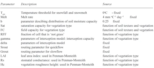
Table 1. Model parameters

Parameter Description Source

Tcrit Temperature threshold for snowfall and snowmelt 0oC - fixed

Melt Melt rate 4 mm o_C–1 _day–1 _fixed

b parameter descibing distribution of soil moisture capacity 0.25 fixed

Sat saturation capacity for vegetation type function of soil texture and vegetation

FC field capacity for vegetation type function of soil texture and vegetation

RFF fraction of cell that is ‘not grass’ function of vegetation type

gamma parameters of interception model: interception capacity function of vegetation type

delta parameters of interception model fixed

Srout routing parameter for quickflow fixed

Grout routing parameter for slowflow fixed

LAI leaf area index: used in Penman-Monteith function of vegetation type

Rs stomatal conductance: used in Penman-Monteith function of vegetation type

The model requires information on field capacity and saturation capacity, both of which are related to soil texture using empirical equations developed by Saxton et al. (1986) and used by Vorosmarty et al. (1989). The geographic distribution of soil texture classes was taken from the FAO Digital Soil Map of the World. The dominant soil class within each 0.5o_{× 0.5}o _{cell was determined by overlaying a}

grid onto the FAO polygon coverage.

VALIDATION OF SIMULATED RUNOFF

Data sources

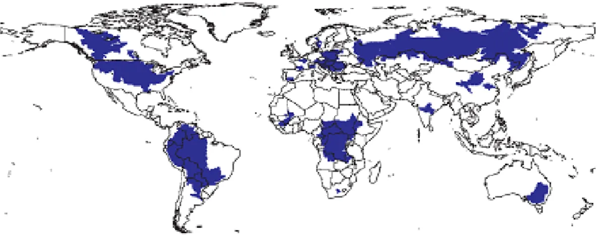
Although model parameters are not calibrated explicitly, some are based on the results of a validation exercise using European data, as described by Arnell (1999c). The ability of the model to simulate river runoff across the globe has been evaluated by comparing model estimates to observed runoff from 50 catchments (Fig. 1) held by the Global Runoff Data Centre (GRDC). Observed runoff was calculated over the period 1961–1990, but record lengths within this period ranged from 10 to 30 years with an average of 22 years. Average annual runoff

Figure 2 shows the relationship between the observed and simulated average annual runoff. The correlation coefficient between the two sets is 0.91, and the median bias is 10%. There are, however, some very large percentage overestimations in dry areas. This is largely because the hydrological model does not incorporate transmission losses along the river channel or evaporation from wetlands and depressions (as noted also by Nijssen et al., 2001 and Döll et al., 2003), but is due partly to the assumption that rain falls everywhere within a grid cell. Simulated runoff is also dependent on the input climatic data. Precipitation is likely to be underestimated in high latitude areas, and the relatively

coarse resolution of the input data also means that runoff will probably be underestimated in areas with large ranges in topography; because of the non-linear linkages between precipitation and runoff, the runoff resulting from the average precipitation will not be the same as the summed runoff resulting from the disaggregated precipitation. Finally, the observations from some of the validation catchments are of unknown quality, and the gauging stations are not necessarily located very close to the catchment outlets.

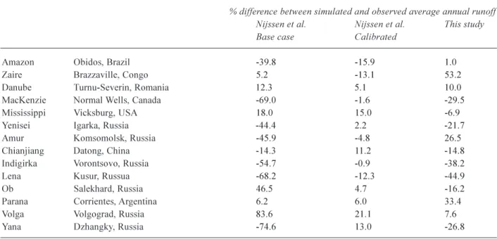
Some of the validation catchments are the same as those used by Nijssen et al. (2001b) and Table 2 compares the bias in estimated average annual runoff using the current (uncalibrated) model with that of Nijssen et al.’s uncalibrated and calibrated models. The current model is usually better than Nijssen et al.’s uncalibrated model, but usually worse than their calibrated model.

Fig. 1. Location of validation catchments

Fig. 2. Observed and simulated average annual runoff (at least 10

Table 2. Comparison with Nijssen et al. (2001b) model performance

% difference between simulated and observed average annual runoff Nijssen et al. Nijssen et al. This study

Base case Calibrated

Amazon Obidos, Brazil -39.8 -15.9 1.0

Zaire Brazzaville, Congo 5.2 -13.1 53.2

Danube Turnu-Severin, Romania 12.3 5.1 10.0

MacKenzie Normal Wells, Canada -69.0 -1.6 -29.5

Mississippi Vicksburg, USA 18.0 15.0 -6.9

Yenisei Igarka, Russia -44.4 2.2 -21.7

Amur Komsomolsk, Russia -45.9 -4.8 26.5

Chianjiang Datong, China -14.3 11.2 -14.8

Indigirka Vorontsovo, Russia -54.7 -0.9 -38.2

Lena Kusur, Russua -68.2 -12.3 -44.9

Ob Salekhard, Russia 46.5 4.7 -16.2

Parana Corrientes, Argentina 6.2 6.0 33.4

Volga Volgograd, Russia 83.6 21.1 7.6

Yana Dzhangky, Russia -74.6 13.0 -26.8

Table 3. Indicators of hydrological behaviour

Indicator Definition Scale

Average annual runoff Average annual runoff calculated over 30 years Catchment

Drought runoff Annual runoff exceeded in 90% of years Catchment

Inter-annual variability in runoff Coefficient of variation of annual total runoff Catchment

Flood runoff 10-year return period maximum monthly runoff 0.5 × 0.5o

Monthly runoff regime Mean monthly runoff 0.5 × 0.5o

Mean monthly runoff

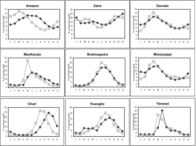
Figure 3 shows the observed and simulated monthly flow regimes for nine catchments (the same as or similar to those used by Nijssen et al., 2001b, in their Fig. 3), with runoff expressed as a percentage of the annual total. The simulated flows are unrouted, and effectively simply summed across all the 0.5o _{× 0.5}o _{grid cells within a catchment. With the}

exception of the Amazon, the simulated flow regimes are similar to the observed ones, although because they are not routed sometimes peak a month in advance. The difference between observed and simulated is greatest in the Amazon basin, because here the routing effect is greatest. The simulated regime has a similar shape to that of Nijssen et al.’s uncalibrated model.

INDICATORS OF HYDROLOGICAL BEHAVIOUR

Several indicators of hydrological behaviour are calculated, as summarised in Table 3. Some of the indicators — average

annual runoff, ‘drought runoff’ and inter-annual variability in runoff — are calculated at the catchment scale, and some — the 10-year return period maximum monthly runoff and mean monthly runoff regime — are calculated at the original 0.5o_{× 0.5}o _{scale. This is because the latter two indicators of}

behaviour are dependent not only on the magnitude of runoff, but on how it is routed along the river network. The 10-year return period maximum monthly runoff is estimated by fitting a generalised extreme value (GEV) distribution to the 30 annual maximum monthly runoff values. The ‘drought runoff’ is equal to the volume of flow exceeded in 90% of years.

Climate change scenarios

SRES EMISSIONS SCENARIOS

The IPCC SRES (Special Report on Emissions Scenarios) emissions scenarios (IPCC, 2000) supercede the IS92a

family of projections used in climate simulations until the late 1990s, and were constructed in a fundamentally different way. The starting point for each projection of future emissions was a ‘storyline’, describing the way world population, economies and political structure may evolve over the next few decades. The storylines were grouped into four scenario families and led, ultimately, to the construction of six SRES marker scenarios (one of the families has three marker scenarios, the others one each). The four families can be characterised briefly as follows:

A1: Very rapid economic growth with increasing globalisation, an increase in general wealth, with convergence between regions and reduced differences in regional per capita income. Materialist-consumerist values predominate, with rapid technological change. Three variants within this family make different assumptions about sources of energy for this rapid growth: fossil intensive (A1FI), non-fossil fuels (A1T) or a balance across all sources (A1B).

B1: Same population growth as A1, but development takes

a much more environmentally-sustainable pathway with global-scale cooperation and regulation. Clean and efficient technologies are introduced. The emphasis is on global solutions to achieving economic, social and environmental sustainability.

A2: Heterogeneous, market-led world, with less rapid economic growth than A1, but more rapid population growth due to less convergence of fertility rates. The underlying theme is self-reliance and preservation of local identities. Economic growth is regionally-oriented and, hence, both income growth and technological change are regionally diverse.

B2: Population increases at a lower rate than A2 but at a higher rate than A1 and B1, with development following environmentally, economically and socially sustainable locally-oriented pathways.

Figure 4 shows the carbon emissions associated with each emissions scenario, together with the change in global temperature under each scenario (assuming one particular energy balance model: IPCC, 2001).

Fig. 3. Observed and simulated runoff regimes in nine catchments: observed dark, simulated light

Observed dark, simulated light

Zaire 0 2 4 6 8 10 12 14 J F M A M J J A S O N D % of annual r unof f Amazon 0 2 4 6 8 10 12 14 J F M A M J J A S O N D % of annual r unof f Danube 0 2 4 6 8 10 12 14 16 J F M A M J J A S O N D % of annual r unof f Mississippi 0 2 4 6 8 10 12 14 16 18 J F M A M J J A S O N D % of annual r unof f Brahmaputra 0 5 10 15 20 25 30 J F M A M J J A S O N D % of annual r unof f MacKenzie 0 5 10 15 20 25 30 35 J F M A M J J A S O N D % of annual r unof f Chari 0 5 10 15 20 25 30 J F M A M J J A S O N D % of annual r unof f Huanghe 0 5 10 15 20 25 J F M A M J J A S O N D % of annual r unof f Yenesei 0 5 10 15 20 25 30 35 40 J F M A M J J A S O N D % of annual r unof f

The most comprehensive set of experiments has been run with HadCM3. This set includes three repetitions of the A2 emissions scenario (known as an ensemble simulation), each starting from a different initial condition, and two repetitions of the B2 emissions scenario. These ensemble scenarios give some indications of the effects of inter-annual climatic variability on the climate change signal.

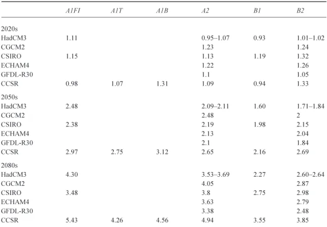
Table 5 shows the change in global average temperature relative to the 1961–1990 average under the climate change scenarios. By the 2080s, the differences in the magnitude of temperature changes as simulated by a given model under the different emissions scenarios are clear, with A1FI producing the greatest increase, followed by A2, A1B, A1T, and B2, while B1 produces the smallest increase. For a given emissions scenario, the CCSR/NIES2 model produces the greatest increase in temperature, and GFDL_R30 the least: under the A2 emissions scenario the difference between the two is 1.6o_{C by the 2080s. (Note that two of the GCMs}

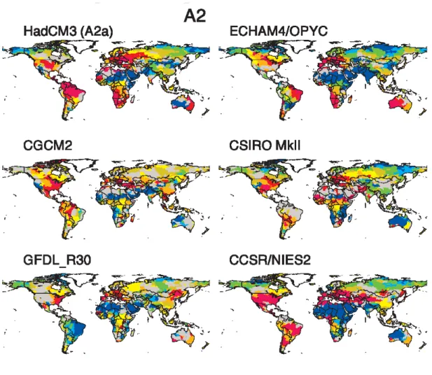
cited in IPCC (2001) but without data on the IPCC-DDC at CRU produce lower increases in temperature than GFDL_R30). In each case, temperature increases are greatest at high latitudes. Figure 5 shows the percentage change in annual precipitation under the A2 emissions scenario and each climate model by the 2050s. The patterns of change for each model are very consistent — suggesting that even by the 2050s the different emissions scenarios produce similar climate changes, and that the broad patterns produced reflect the atmospheric forcing rather than climatic variability — and there is a strong degree of consistency between the climate models. This has been explored in more detail by Giorgi et al. (2001), who showed very considerable consistency in patterns of regional climate change over the 21st century.

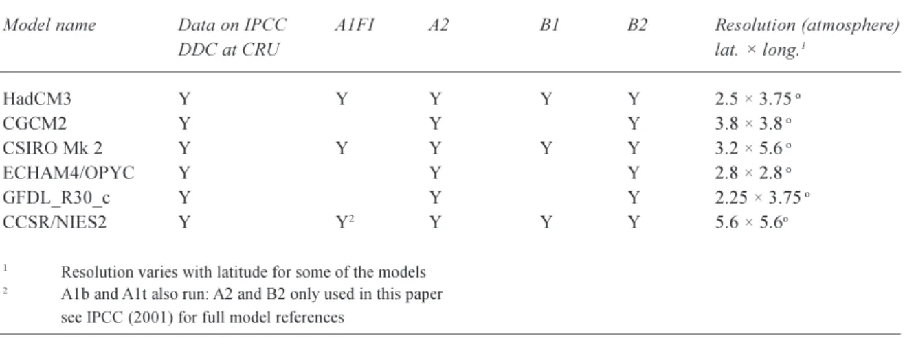
Table 4. Summary of climate change experiments using the SRES emissions scenarios, with summary data on the

IPCC-DDC emissions

Model name Data on IPCC A1FI A2 B1 B2 Resolution (atmosphere)

DDC at CRU lat. × long.1

HadCM3 Y Y Y Y Y 2.5 × 3.75 o CGCM2 Y Y Y 3.8 × 3.8 o CSIRO Mk 2 Y Y Y Y Y 3.2 × 5.6 o ECHAM4/OPYC Y Y Y 2.8 × 2.8 o GFDL_R30_c Y Y Y 2.25 × 3.75 o CCSR/NIES2 Y Y2 _{Y Y Y 5.6 × 5.6}o

1 _{Resolution varies with latitude for some of the models} 2 _{A1b and A1t also run: A2 and B2 only used in this paper}

see IPCC (2001) for full model references Fig. 4 Global emissions and changes in average temperature

associated with each SRES emissions scenario

CLIMATE SCENARIOS

The effects of these emissions scenarios on regional climates have been determined using a number of global climate models. The Third Assessment Report of the IPCC (IPCC, 2001) describes the results from nine climate models run with two or more of the SRES emissions scenarios: these models are summarised in Table 4. Data for all the model runs are held at the IPCC’s Data Distribution Centre, and summary data for six (indicated in Table 4) are available (as of May 2003) from the DDC website at the Climatic Research Unit (ipcc-ddc.cru.uea.ac.uk). Only the six models for which summary data were available were used in the current study.

Temperature change: IPCC SRES scenarios

0 1 2 3 4 5 1990 2000 2010 2020 2030 2040 2050 2060 2070 2080 2090 2100 oC r e la ti ve t o 1990

APPLYING SCENARIOS

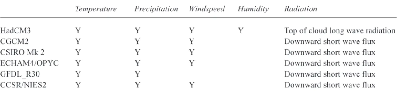
Table 6 shows the variables available for each climate model: all were expressed as 30-year monthly mean values, calculated for the baseline period (1961–1990), the 2020s (2010–2039), the 2050s (2040–2069) and the 2080s (2070– 2099). Each climate model provided changes in monthly mean precipitation and temperature, and all but GFDl-R30 provided windspeed. Change in vapour pressure was only available for the HadCM3 simulations, so for the other climate models it was assumed that relative humidity remained constant and future vapour pressure was estimated from future temperature and baseline relative humidity. None of the scenario sets provides data on net radiation at the surface, and approximate procedures had to be applied to create net radiation scenarios. Net radiation under the HadCM3 scenarios was estimated by assuming that top of cloud long wave radiation (tclw) was a surrogate for cloud cover, applying changes in tclw to CRU observed cloud cover data, and calculating net radiation using standard empirical formulae (Shuttleworth, 1993). Net radiation under the CSIRO, CGCM2, ECHAM4, GFDL-R30 and CCSR/NIES2 scenarios was determined by applying the

changes in surface short-wave radiation to baseline downward short-wave radiation (estimated using standard empirical formulae) and calculating changes in net long-wave radiation due to changes in temperature and humidity (again using standard formulae).

The changes in the mean monthly climate variables were applied to the CRU 0.5o_{× 0.5}o _{1961–1990 monthly time}

series (New et al., 1999) to create perturbed 30-year time series representing climate around the three study time horizons (2020s, 2050s and 2080s). Changes to precipitation and windspeed were applied as percentages, whilst changes to temperature, vapour pressure and net radiation were applied in absolute terms. Because the same changes were applied to each year of the 30-year baseline time series, the relative variability in climate from year to year remains unchanged. In particular, the coefficient of variation of monthly rainfall remains constant. No changes were made to the daily sequencing of rainfall and temperature.

The GCM resolution scenarios were applied by making the same percentage or absolute changes to all the 0.5o_{× 0.5}o

grid cells lying within an individual GCM grid cell. The resulting changes in climate vary across each GCM grid

Table 5. Increase in global average temperature (o_{C) relative to 1961–1990}

A1FI A1T A1B A2 B1 B2

2020s HadCM3 1.11 0.95–1.07 0.93 1.01–1.02 CGCM2 1.23 1.24 CSIRO 1.15 1.13 1.19 1.32 ECHAM4 1.22 1.26 GFDL-R30 1.1 1.05 CCSR 0.98 1.07 1.31 1.09 0.94 1.33 2050s HadCM3 2.48 2.09–2.11 1.60 1.71–1.84 CGCM2 2.48 2 CSIRO 2.38 2.19 1.98 2.15 ECHAM4 2.13 2.04 GFDL-R30 2.1 1.84 CCSR 2.97 2.75 3.12 2.65 2.16 2.69 2080s HadCM3 4.30 3.53–3.69 2.27 2.60–2.64 CGCM2 4.05 2.87 CSIRO 3.48 3.8 2.75 2.98 ECHAM4 3.63 2.79 GFDL-R30 3.38 2.48 CCSR 5.43 4.26 4.56 4.94 3.55 3.85

Table 6. Variables from the climate change experiments

Temperature Precipitation Windspeed HumidityRadiation

HadCM3 Y Y Y Y Top of cloud long wave radiation

CGCM2 Y Y Y Downward short wave flux

CSIRO Mk 2 Y Y Y Downward short wave flux

ECHAM4/OPYC Y Y Y Downward short wave flux

GFDL_R30 Y Y Downward short wave flux

CCSR/NIES2 Y Y Y Downward short wave flux

All variables presented as monthly mean values calculated over 30 years

cell (all 0.5o_{× 0.5}o _{cells have the same changes in monthly}

precipitation, for example, but effects on annual precipitation depend on the distribution of precipitation through the year in the individual cells), but there are still some discontinuities at GCM cell boundaries.

More sophisticated spatial and temporal downscaling techniques could, in principle, have been applied, but they would have required calibration for each of the 65 000 0.5o_{× 0.5}o _{grid cells and would have simply added smoothed}

detail to the initial GCM climate changes.

Changes in potential evaporation are driven by changes in temperature, net radiation, vapour pressure and windspeed. In practice, changes in windspeed have relatively little effect, and changes in temperature have a greater effect on potential evaporation than changes in net radiation. Under the HadCM3 scenarios, relative humidity decreases across much of the world but increases in some areas, particularly at high latitudes, and has a large effect on potential evaporation. The assumption that relative humidity remains constant for the other scenarios, therefore, tends to mean that they result in smaller increases in potential evaporation than the HadCM3 scenarios.

Catchment vegetation properties (leaf area index, interception storage capacity and root depth) were assumed constant over all simulations, and it was assumed that the net effect of CO2 enrichment on evaporation is negligible at the catchment scale. Reductions in stomatal conductance are assumed to be offset by increases in plant leaf area. Catchment land cover is also assumed unchanged.

Natural multi-decadal climatic

variability

CLIMATIC ANOMALIES DUE TO MULTI-DECADAL VARIABILITY

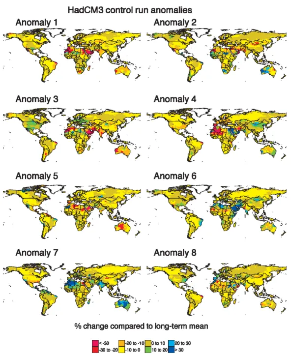
Climate change due to increasing concentrations of greenhouse gases must be seen in the context of natural multi-decadal variability. A long ‘control-run’ experiment has been run with HadCM3 (Gordon et al., 2000), starting from 1860 and finishing in 2100, assuming no change in greenhouse gas concentrations. Eight scenarios for 30-year mean monthly temperature and precipitation were constructed from this long control run, starting with the period 1860–1889. The precise pattern of multi-decadal variability depends of course on which 30-year period is taken as the baseline, but the maximum temperature anomaly over land is always less than ±1o_{C, with all but high latitudes}

generally showing anomalies of less than 0.25o_{C. The natural}

multi-decadal variability effect on mean temperature is therefore considerably smaller than the climate change

effect, under all the emissions scenarios, at least from the 2050s. The 30-year mean annual precipitation anomalies are less than 10% in all but very arid areas, and individual anomaly patterns are very different from those caused by climate change: there is no clear latitudinal variability as shown in Fig. 5.

These eight sets of 30-year mean monthly temperature and precipitation were expressed as departures from the simulated 1961–1990 average, to create eight ‘natural variability’ scenarios. It was assumed that windspeed, net radiation and relative humidity remained constant in each scenario.

VARIABILITY IN AVERAGE ANNUAL RUNOFF

These eight scenarios were used to create eight sets of simulated 30-year hydrological time series. Figure 6 shows the change in catchment average annual runoff under the natural variability scenarios, expressed as a change from the average calculated over all eight scenarios (in other words, the anomaly between each 30-year mean and the mean calculated over 240 years), and is indicative of the types of spatial pattern of change in runoff due to multi-decadal variability: anomalies calculated with respect to individual 30-year periods can be larger than those shown in Fig. 6, particularly in dry regions.

One measure of multi-decadal variability in a catchment is the standard deviation of anomalies, but this varies depending on which time period is used as the baseline. Figure 7 shows the average standard deviation of percentage change in average annual runoff, calculated using each of the eight 30-year time periods successively as the baseline period. This is less than 10% across most of the world, but is higher in drier catchments.

Effect of climate change

AVERAGE ANNUAL CATCHMENT RUNOFF

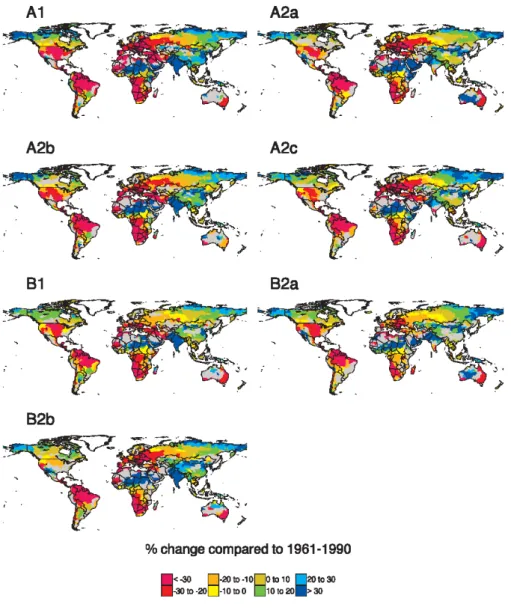
Figure 8 shows the percentage change in average annual catchment runoff by the 2050s, under the seven HadCM3-based scenarios, with changes less than the standard deviation of 30-year average annual runoff (Fig. 7) shown in grey. Figure 9 shows the change in average annual catchment runoff by the 2050s with all six climate models and the A2 emissions scenario. By the 2020s approximately a third of all catchments have a ‘substantial’ (i.e. greater than the standard deviation) increase in runoff, a third have a substantial decrease, and a third show no substantial change (Table 7). By the 2050s the number with no substantial change reduces to between 20 and 30%, and it falls to between 10 and 30% by the 2080s. The HadCM3 patterns

Fig. 6. Percentage change in 30-year average annual runoff due to natural multi-decadal climatic variability

shown in Fig. 8 are broadly similar to those produced when HadCM3 was run with the IS92a emissions scenario (Arnell, 1999a), although they are more similar to each other than to the IS92a pattern: this is largely because the SRES emissions scenarios include sulphate emissions whilst the simulation with the IS92a emissions scenario did not.

A visual inspection of Figs. 8 and 9 suggests that there is a generally strong degree of consistency in change in runoff, with little difference in the pattern of change between emissions scenarios. Table 8 shows the correlations between all the simulated absolute changes in runoff by the 2050s

across the 1163 catchments (unweighted by catchment area). For each climate model, correlations are generally very high between runs with different emissions scenarios, suggesting that the projected pattern of change for a given model varies little between emissions scenario. Within the HadCM3 scenario set, there is no clear difference in correlations within the two groups of ensemble members (A2a, A2b and A2c, and B2a and B2b) and amongst all seven scenarios. Correlations between climate models are generally weaker than correlations between emissions scenarios; the closest correspondences were between HadCM3 and ECHAM4.

Fig. 7. Standard deviation of percentage change in average annual runoff, calculated as the average using each of the 30-year time periods

successively as the baseline period

Fig. 9. Percentage change in average annual runoff by the 2050s: A2 emissions

Figure 10 shows the degree of consistency in the estimated direction of change in average annual runoff across the eight simulations using the A2 emissions scenario (three HadCM3 runs, with one each from ECHAM4, CSIRO, CGCM2, GFDL_R30 and CCSR/NIES2). Areas where more than half of the simulations show a significant decrease in runoff (greater than the standard deviation of natural multi-decadal variability) include much of Europe, the Middle East, southern Africa, North America and most of South America. Areas with consistent increases in runoff include high latitude North America and Siberia, eastern Africa, parts of arid Saharan Africa and Australia, and south and east Asia. Correlations and consistency maps, however, only take into account the pattern of change, and not its magnitude. It can be expected from Fig. 4 that, for a given climate model

and location, the magnitude of change should be decrease from A1FI through A2 and B2, with the smallest changes under B1 and the divergence increasing from the 2020s to the 2080s. More specifically, it can be hypothesised that the greatest range in change in average annual runoff across the world will occur under A1FI (the greatest increases and the greatest decreases), and the smallest range will occur under B1. A good generalised measure of the variability in change in runoff across the world is its standard deviation. Percentage changes in runoff across the 1163 catchments are highly skewed with some very large percentage changes in dry areas, so Fig. 11 shows the standard deviation in absolute change across the 1163 catchments. By the 2020s there is little difference in standard deviation with emissions scenario (for a given climate model), implying that not only

Table 7. Percentage of catchments with increase or decrease in average annual runoff

2020 2050 2080

increase no change decrease increase no change decrease increase no change decrease

HadCM3-a1 40 31 29 40 18 41 42 10 48 HadCM3-a2a 34 32 33 40 21 39 39 14 47 HadCM3-a2b 39 31 30 40 19 42 40 13 47 HadCM3-a2c 33 32 35 38 21 42 40 12 48 HadCM3-b1 36 33 31 36 23 40 40 19 41 HadCM3-b2a 38 30 32 41 22 37 41 18 41 HadCM3-b2b 38 34 28 42 24 34 42 18 39 CSIRO-a1 33 41 26 39 29 32 42 24 34 CSIRO-a2 37 40 22 40 30 31 43 20 37 CSIRO-b1 39 37 25 40 28 31 42 27 32 CSIRO-b2 36 36 28 42 32 26 42 24 34 CGCM-a2 32 38 30 27 27 45 23 22 55 CGCM-b2 29 36 35 26 37 37 24 29 47 ECHAM4-a2 42 25 33 43 20 37 49 13 38 ECHAM4-b2 42 26 32 45 19 37 45 17 38 GFDL-a2 46 35 19 46 25 30 52 19 29 GFDL-b2 44 36 20 43 32 25 48 27 25 CCSR-a2 35 33 32 46 12 42 45 9 46 CCSR-b2 39 29 33 48 15 37 44 14 42

Note: “increase” and “decrease” denote changes greater than the standard deviation of natural multi-decadal variability in average annual runoff

Table 8. Correlation between absolute change in average annual runof f across 1163 catchments

is largely determined by the pattern of change in precipitation, tempered by variations in the increase in potential evaporation. Figure 12 shows the change in annual runoff by the 2050s under the HadCM3 scenario, assuming (i) change in precipitation and potential evaporation, (ii) change in precipitation only and (iii) change in potential evaporation only. In effect, the increase in potential evaporation reduces increases in runoff due to higher precipitation in some areas — principally high latitudes — and more than offsets the effect of an increase in precipitation in many mid-latitude areas such as large parts of North America and Europe.

CHANGE IN VARIABILITY IN FLOW FROM YEAR TO YEAR

The climate change scenarios used in this study assume no change in the relative variability in climate from year to year. Nevertheless, because of the non-linear linkages between rainfall and runoff, the scenarios may result in changes in the relative variability in flows from year to year. The coefficient of variation (CV) of catchment annual runoff varies geographically, ranging from around 0.2 in humid regions to between 0.6 and 1.0 in dry parts of southern Africa and Australia (the CV in annual runoff at smaller spatial scales is larger). Natural multi-decadal variability results in differences in the CV of annual runoff from the 1961–1990 baseline of less than 4% across much of the world, but ranging up to 15% in dry regions.

Figure 13 shows the effect of the HadCM3 scenarios on the CV of catchment annual runoff by the 2050s, and shows that climate change generally increases the relative variability of runoff by more than would be expected due to natural multi-decadal climatic variability. The HadCM3 scenarios, for example, result in increases in CV of around 15% across much of Europe and western Russia, and around 25% in the Amazon basin. CV decreases by up to 10% in a few catchments in western and northern Africa and, under some emissions scenarios, central North America. There is no apparent general relationship between the direction of change in mean runoff and the direction of change in CV, and the change is CV is related more to how the high and low annual runoff extremes are altered by climate change. The decrease in CV in central North America under some scenarios, for example, occurs because the largest annual runoff value is reduced by considerably more than the mean.

CHANGE IN THE FREQUENCY OF CATCHMENT ‘DROUGHT’ RUNOFF

Changes in average catchment runoff (Fig. 8), together with changes in the relative variability of catchment runoff from are the patterns of change similar between the emissions

scenario, but the magnitudes of change are similar too. By the 2050s, there is still little clear difference between the emissions scenarios for CSIRO, but some suggestions with HadCM3 that A1FI produces the greatest and B1 the smallest effect, and with GFDL_R30 that A2 has a greater effect than B2. By the 2080s, there is a clear gradation from A1FI through A2 and B2 to B1 with HadCM3, and clear differences between A2 and B2 for the other models.

The spatial pattern of change in runoff for a given scenario

2050 s Had CM3 -a1 Had CM 3-a 2a Had CM3 -a 2b Had CM 3-a 2c Had CM 3-b 1 Had CM3 -b 2a Had CM 3-b 2b CSIRO -a 1 CSIRO -a 2 CS IRO-b1 CS IRO-b2 CGCM -a2 CGCM -b 2 ECH AM 4-a 2 ECH AM 4-b 2 GFDL -a 2 GFDL -B 2 CCSR-A 2 CCS R-B 2 H a d C M 3 -a 1 1. 0 0 H a dC M 3 -a 2a 0 .89 1.0 0 H adC M 3 -a 2 b 0. 9 7 0 .87 1. 0 0 H a dC M 3 -a 2c 0 .91 0.9 3 0 .91 1 .00 H a dCM 3 -b1 0 .93 0.8 5 0 .95 0 .90 1.0 0 H adC M 3 -b 2 a 0. 8 5 0 .93 0. 8 4 0. 8 8 0 .81 1. 0 0 H ad C M 3 -b 2b 0 .95 0.9 0 0 .95 0 .91 0.9 3 0 .83 1.0 0 C S IR O -a 1 0. 3 1 0 .15 0. 3 3 0. 1 8 0 .25 0. 2 3 0 .21 1. 0 0 CS IR O -a 2 0 .10 0.0 5 0 .13 0 .07 0.1 1 0 .09 0.0 6 0 .77 1.0 0 CS IR O -b1 0 .26 0.0 5 0 .26 0 .12 0.2 0 0 .13 0.1 3 0 .83 0.6 9 1 .00 CS IR O -b2 0 .20 0.0 8 0 .24 0 .13 0.2 0 0 .17 0.1 2 0 .86 0.8 6 0 .81 1.0 0 CG CM -a 2 0. 3 2 0 .38 0. 2 7 0. 3 3 0 .27 0. 3 4 0 .35 0. 0 9 0 .06 0. 1 0 0 .04 1 .00 CG C M -b 2 0. 4 2 0 .44 0. 4 0 0. 4 1 0 .37 0. 3 5 0 .45 0. 1 6 0 .11 0. 2 0 0 .09 0 .84 1. 0 0 E C H A M 4 -a 2 0. 4 6 0 .36 0. 4 0 0. 3 7 0 .38 0. 3 8 0 .38 0. 2 1 -0 .0 1 0. 2 1 0 .07 0 .28 0. 1 8 1. 0 0 E C H A M 4 -b 2 0. 4 5 0 .34 0. 3 9 0. 3 5 0 .38 0. 3 4 0 .37 0. 2 2 0 .01 0. 2 5 0 .09 0 .28 0. 2 1 0. 9 4 1 .00 G F D L -a 2 -0 .3 9 -0 .4 4 -0 .3 6 -0 .4 7 -0 .3 8 -0 .3 8 -0 .3 8 0. 1 1 0 .13 0. 1 6 0 .15 -0 .0 9 -0 .0 5 -0 .2 0 -0 .1 4 1 .00 G F D L -B 2 -0 .3 4 -0 .4 2 -0 .3 3 -0 .4 2 -0 .3 3 -0 .3 0 -0 .3 6 0. 0 7 0 .04 0. 1 4 0 .09 -0 .1 4 -0 .0 8 -0 .2 0 -0 .1 4 0 .75 1. 0 0 CC S R -A 2 0 .30 0.2 4 0 .30 0 .27 0.2 4 0 .25 0.2 5 0 .28 0.1 2 0 .22 0.1 9 0.2 5 0 .25 0 .23 0.2 0 -0.0 1 -0 .08 1. 00 CCS R-B2 -0 .02 -0.1 2 0 .01 -0 .06 -0.0 6 -0 .08 -0.0 7 0 .22 0.0 9 0 .19 0.1 6 0.0 5 0 .10 -0 .03 -0.0 6 0.2 7 0 .17 0. 83 1.0 0

Fig. 11. Standard deviation of absolute change in average annual runoff across the 1163 catchments, by scenario and time horizon

Standard deviation (mm) of catchment runoff change: 2020s

0 10 20 30 40 50 60 70 80 90 100 Ha dCM 3 -a 1 H a dC M3 -A 2 H a dC M3 -A 2 H a dC M3 -A 2 Ha dc m 3 -B 1 Ha dc m 3 -B 2 Ha dc m 3 -B 2 CS IRO -A 1 CS IRO -A 2 CS IRO -B 1 CS IRO -B 2 CG CM -A 2 CG CM -B 2 EC H A M 4 -A 2 EC H A M 4 -B 2 GF D L -A 2 GFD L -B 2 CCS R-A 2 CC S R -B 2 s d ( m m c h ang e)

Standard deviation (mm) of catchment runoff change: 2050s

0 20 40 60 80 100 120 140 160 180 200 Had C M3 -a 1 Ha dCM 3 -A 2 Ha dCM 3 -A 2 Ha dCM 3 -A 2 Had c m 3 -B 1 Ha dc m 3 -B 2 Ha dc m 3 -B 2 CS IRO -A 1 CS IRO -A 2 CS IR O -B 1 CS IR O -B 2 CG C M -A 2 CG C M -B 2 E CHA M 4 -A 2 E CHA M 4 -B 2 GFD L -A 2 GF D L -B 2 CC S R -A 2 CC S R -B 2 sd (m m ch a n g e )

Standard deviation (mm) of catchment runoff change: 2080s

0 50 100 150 200 250 300 Ha dCM 3 -a 1 H a dC M 3 -A 2 H a dC M 3 -A 2 H a dC M 3 -A 2 Ha dc m 3 -B 1 H a dc m 3 -B 2 H a dc m 3 -B 2 CS IR O -A 1 CS IR O -A 2 CS IRO -B 1 CS IRO -B 2 CG CM-A 2 CG CM -B 2 EC H A M 4 -A 2 EC H A M 4 -B 2 GF D L -A 2 GF D L -B 2 CCS R -A 2 CCS R-B 2 s d ( mm c h an ge)

year to year (Fig. 13), mean that the frequency of occurrence of “drought” river flows is likely to change in the future. The rather crude indicator of drought used in this study is the 10-year return period annual minimum catchment runoff: catchment runoff is below this value in 10% of years.

The top part of Fig. 14 shows the pattern of change in drought runoff under two scenarios — HadCM3-A2a and HadCM3-B2a — by the 2050s. These patterns of change are similar to the change in average annual catchment runoff, although the percentage changes are slightly greater. The bottom part of Fig. 14 shows the percentage of years that watershed annual runoff is less than the baseline drought runoff for the same two scenarios. Where the percentage is less than 10% droughts are less common that at present. Under these scenarios, the percentage of years with runoff below the current drought runoff is increased to around 30% across much of southern Africa, Europe and the Amazon basin (a factor of three increase), and to around 20% across large parts of North America.

CHANGES IN FLOW TIMING

A change in climate has the potential to alter the timing of flows through the year, as well as the magnitude of flows and the range between high and low flows. This change in timing may occur because the timing of the rainy season alters, or — more generally — because the proportion of precipitation falling as snow, and hence being stored on the catchment, declines due to higher temperatures.

Figure 15 shows the mean monthly runoff regimes for a number of 0.5o_{× 0.5}o _{grid cells, under the baseline climate}

and the HadCM3 A1FI scenario for the 2050s (the same cells were shown in Arnell (1999b)). The two cells with maritime climates — southern England and Italy — show little change in the timing of flows through the year, but an increase in the seasonal variation, particularly in the English cell. There is a substantial change in the timing of flow in the cells in Belarus and the north east USA, with large increases in winter runoff and the snowmelt-induced peak moving a month earlier. This is less apparent in the Great Plains cell, and the month of maximum runoff does not change in the west Russian cell. In these two cases, winter temperatures are so low that increasing temperatures do not result in significantly earlier snowmelt. The other cells show no clear change in the timing of maximum or minimum runoff. Similar patterns are found with the other climate models, although the magnitudes of change in monthly runoff differ.

CHANGE IN MAXIMUM MONTHLY RUNOFF

The 10-year return period maximum monthly runoff, estimated from the 0.5o_{× 0.5}o _{data by fitting a general}

extreme value (GEV) distribution, was used as a generalised measure of ‘flood’ magnitudes. In practice, flood peak values are not necessarily closely correlated with monthly runoff totals, but changes in the magnitude of the 10-year maximum monthly runoff do give an indication of potential changes in flood magnitude. In the hydrological simulations, daily rainfall is generated stochastically from monthly rainfall, given an estimate of the number of days rain falls in a month. The estimated number of rain-days is assumed unchanged

Fig. 12. Percentage change in average annual runoff by the 2050s, under the HadCM3 A2a scenario, assuming (i) change in precipitation and

in all simulations (because the scenarios give no information on changes), and the effects of a constant or increasing amount of rain falling on fewer rain days are not accounted for. The modelling approach adopted therefore is likely to underestimate the effect of climate change on flood flows, particularly where the climate change has a large effect on rainfall frequency.

The spatial pattern of change in the 10-year maximum monthly runoff is broadly similar to the pattern of change in average annual runoff (see Fig. 16 for two scenarios),

Fig. 13. Percentage change in the coefficient of variation of catchment annual runoff by the 2050s (HadCM3)

although the relationships between the percentage changes depend on how rainfall changes through the year. For example, flood magnitudes are reduced more when rainfall falls throughout the year than when a decrease in rainfall in one season is partially offset by an increase in the flood-generating season. Changes in flood magnitude are small relative to natural multi-decadal variability across much of Europe, and reductions in flood peaks are much smaller than the reductions in average runoff across Amazonia.

Fig. 14. Change in ‘drought’ runoff: percentage change in 10-year return period annual runoff, and percentage of years that watershed annual

runoff is below the current 10-year return period annual runoff

Conclusions

CAVEATS

This paper describes an analysis of the implications of the IPCC SRES emissions scenarios for river flows across the world, using a number of climate models to create scenarios for change in climate which are then fed into a macro-scale hydrological model operating at a spatial resolution of 0.5o_{× 0.5}o_{. Before summarising the key conclusions and}

implications, it is important to review the limitations of the study.

These fall into two main categories, concerning the climate change scenarios and the hydrological model. The key caveats associated with the climate change scenarios are:

l The scenarios represent just the change in monthly mean

climate: changes in year-to-year variability can be expected to occur and to influence changes in both mean and extreme streamflows.

l The scenarios have not been interpolated down to the

0.50o_{× 0.5}o _{resolution used in the hydrological model,}

so there are some discontinuities at GCM cell boundaries.

l The scenarios that do not specify changes in relative

humidity tend to produce smaller increases in potential evaporation than those that do.

The key caveats associated with the hydrological model are:

l A sensitivity analysis exploring the implications of

model parameter uncertainty on projected changes in river flows has not been carried out. However, an analysis using an earlier version of the model at the European scale (Arnell, 1999b) showed the simulated changes in streamflow are relatively insensitive to different values of model parameters, except in semi-arid and semi-arid areas. Estimated changes in runoff in these regions are therefore most uncertain.

l The calculations assumed no net direct effect of CO₂

enrichment on evaporation at the catchment scale. This assumption is justifiable at present, but CO2 enrichment

could reduce catchment evaporative demands, leading to smaller reductions in runoff and greater increases in runoff than simulated in the present analysis.

Fig. 15. Average monthly runoff under current and 2050s climates (HadCM3-A1FI) for individual grid cells SE England 0 10 20 30 40 50 J F M A M J J A S O N D Italy 0 10 20 30 40 50 J F M A M J J A S O N D Belarus 0 10 20 30 40 50 60 J F M A M J J A S O N D W Russia 0 10 20 30 40 50 60 J F M A M J J A S O N D Thailand 0 50 100 150 200 J F M A M J J A S O N D E China 0 20 40 60 80 100 120 140 J F M A M J J A S O N D Great Plains 0 2 4 6 8 10 12 J F M A M J J A S O N D NE USA 0 20 40 60 80 100 120 140 160 J F M A M J J A S O N D SE Brazil 0 50 100 150 200 J F M A M J J A S O N D Ghana 0 10 20 30 40 50 60 J F M A M J J A S O N D South Af rica 0 5 10 15 20 25 30 J F M A M J J A S O N D Tanzania 0 50 100 150 200 250 J F M A M J J A S O N D

Fig. 16. Percentage change in the 10-year return period maximum monthly runoff

transmission losses along arid-zone river channels or the evaporation of water that flows into internal drainage areas, and thus tends to overestimate runoff in dry regions: it therefore overestimates runoff in these areas and underestimates the percentage effect of climate change on the amount of water in rivers in these areas. Finally, the model does not include a glacier melt component, so underestimates future runoff in catchments below melting glaciers.

l The potential additional effects of land cover change

over the next few decades are not included. These trends will of course depend on the socio-economic characteristics associated with each storyline and emissions scenario.

l The model probably underestimates the effects of climate change on high flow magnitudes, partly due to the monthly resolution of the output streamflow and

partly because the potential effects of changes in the number of rain days and intense rainfalls are not incorporated. Simulated changes in monthly mean and annual runoff are the most credible.

l The simulated runoff is not routed along the river

network, because the aim of the study is to determine the spatial pattern of the effects of climate change, not to estimate streamflows at defined locations along a river.

GENERALISED CONCLUSIONS AND IMPLICATIONS

By the 2020s, the effects of climate change on average annual runoff are typically greater than the effects of natural multi-decadal variability in approximately two-thirds of the world, and by the 2080s this has increased to between 70 and 90%. The comparison between the effects of climate change and multi-decadal variability allows the

identification of regions which might be expected to feel the effects of climate change earliest.

The different climate models and emissions scenarios explored produce broadly consistent changes in runoff, with increases in high latitudes, east Africa and south and east Asia, and decreases in southern and eastern Europe, western Russia, north Africa and the Middle East, central and southern Africa, much of North America, most of South America, and south and east Asia. These conclusions are broadly consistent with those of other studies which have examined rivers world-wide (e.g. Nilsson et al., 2001a; Smith and Lazo, 2001). There is little difference in the pattern of change in runoff between the four SRES emissions scenarios considered, for a given climate model, even by the 2080s, and the greatest differences in pattern are between climate models. There is little difference in the magnitudes of change in average annual runoff by the 2050s, and only with the HadCM3 scenarios is it possible to show that the A1FI scenario has the greatest effect, followed by A2, then B2 and finally B1. The limited differences between the emissions scenarios, for a given climate model, implies that — at least until the 2050s — all experiments with a given climate model can be seen as an ensemble of simulations, regardless of actual emissions scenario used.

The spatial pattern of change in runoff for a given scenario is largely driven by the pattern of change in precipitation, modified by the effect of the consistent increase in potential evaporation. In high latitude areas the effect of the higher potential evaporation is to reduce increases in runoff. In mid-latitude areas increases in potential evaporation more than offset the effects of increased precipitation.

Even though the climate scenarios assumed no change in the relative variability of input precipitation, the coefficient of variation of annual runoff increased in most catchments under most scenarios, due to the non-linear linkages between precipitation and runoff. Changes in CV were most influenced by changes in the magnitude of the extreme high and low runoff years. Where average annual runoff decreased, the frequency with which annual runoff was below the current 10-year return period minimum runoff increased substantially, and by the 2050s runoff would be below this ‘drought’ runoff around three times more frequently in parts of Europe and southern Africa, and twice as frequently across much of North America.

The most widespread effect of climate change on river flows is to change the volume of flows and the range in seasonal variability, with the magnitude of change in any one catchment varying considerably between climate models. Across substantial parts of the northern hemisphere increased temperatures mean that a smaller proportion of precipitation falls as snow and that the season of peak flows

is brought forward from spring to winter. This effect is greatest in the marginal zone between cold dry continental regions (where most precipitation still falls as snow by the end of the 21st century) and milder regions where currently little precipitation falls as snow. It results in a large flow regime shift across eastern Europe, mid-latitude North America and the northern parts of east Asia. This change in timing is broadly consistent between climate models, as it depends on temperature rather than precipitation changes. The approach and hydrological model are less suitable for estimating changes in high flows, but the model results indicate that the broad pattern of change in flood peaks will follow the change in average runoff. There are, however, parts of the world — Amazonia and parts of Europe, for example — where a reduction in annual runoff is not accompanied by a similar reduction in flood magnitudes

The implications of these changes in runoff for global and regional water resources are examined in Arnell (2003).

Acknowledgements

This paper is based on work funded by the UK Department for the Environment, Food and Rural Affairs (DEFRA), project number EPG/1/1/70. Climate baseline data and HadCM3 climate change scenarios were provided through the Climate Impacts LINK project by Dr David Viner. The other climate scenarios were taken from the IPCC Data Distribution Centre website ipcc-ddc.cru.uea.ac.uk.

References

Adam, J.C. and Lettenmaier, D.P., 2003. Adjustment of global gridded precipitation for systematic bias. J. Geophys.

Res.-Atmos., 108 (D9), art. no. 4257.

Arnell, N.W., 1999a. Climate change and global water resources.

Global Environ. Change 9, S31–S49.

Arnell, N.W., 1999b. The effect of climate change on hydrological regimes in Europe: a continental perspective. Global Environ.

Change 9, 5–23.

Arnell, N.W., 1999c. A simple water balance model for the simulation of streamflow over a large geographic domain. J.

Hydrol., 217, 314–335.

Arnell, N.W., 2004. Climate change and global water resources: SRES emissions and socio-economic scenarios. Global Environ.

Change. In press.

Arnell, N.W., Liu, C. et al., 2001. Hydrology and water resources.

Climate Change 2001: Impacts and Adaptations. Contribution of Working Group II to the Third Assessment Report of the Intergovernmental Panel on Climate Change, J. McCarthy and

O. Canziani (Eds.). Cambridge University Press, Cambridge, UK.

Arora, V.K. and Boer, G.J., 2001. Effects of simulated climate change on the hydrology of major river basins. J. Geophys.

Res., 106, 3335–3348.

Döll, P., Kaspar, F. and Lehner, B., 2003. A global hydrological model for deriving water availability indicators: model tuning and validation. J. Hydrol., 270, 105–134.

Giorgi, F., Whetton, P.H. et al., 2001. Emerging patterns of simulated regional climate changes for the 21st century due to anthropogenic forcings. Geophy. Res. Letters 28, 3317–3320. Gordon, C., Cooper, C. et al., 2000. imulation of SST, sea-ice

extents and ocean heat transports in a coupled model without flux adjustments. Climate Dynamics 16, 147–168.

IPCC (Intergovernmental Panel on Climate Change), 2000. Special

Report on Emissions Scenarios. Cambridge University Press,

Cambridge, UK.

IPCC, 2001. Climate Change 2001: The Science of Climate

Change. Report of Working Group 1 to the Third Assessment

Report of the Intergovenmental Panel on Climate Change. Cambridge University Press, Cambridge.

New, M., Hulme, M. and Jones, P.D., 1999. Representing twentieth century space-time climate variability. Part 1: development of a 1961-1990 mean monthly terrestrial climatology. J. Climate,

12, 829–856.

Nijssen, B., O’Donnell, G.M., Hamlet, A.F. and Lettenmaier, D.P., 2001a. Hydrologic sensitivity of global rivers to climate change.

Climatic Change 50, 143–175.

Nijssen, B., O’Donnell, G.M., Lettenmaier, D.P., Lohmann, D. and Wood, E.F., 2001b. Predicting the discharge of global rivers.

J. Climate, 14, 3307–3323.

Saxton, K.E, Rawls, W.J., Romberger, J.S. and Papendick, R.I., 1986. Estimating generalised soil water characteristics from texture. Trans. Am. Soc. Agric. Engrs., 50, 1031–1035. Shuttleworth, W.J., 1993.. Evaporation. Handbook of Hydrology,

D.R. Maidment (Ed.). McGraw Hill, New York. 4.1–4.53. Smith, J.B. and Lazo, J.K., 2001. A summary of climate change

impact assessments under the US Country Studies Programme.

Climatic Change, 50, 1–29.

Vorosmarty, C.J., Moore, B., Grace, A.L. et al., 1989, Continental scale models of water balance and fluvial transport: an application to South America. Global Biogeochem. Cycles 3, 241–265.

Vorosmarty, C.J., Green, P., Salisbury, J. and Lammers, R.B., 2000. Global water resources: vulnerability from climate change and population growth. Science, 289, 284–288.