PSFC/RR-05-3
DKE: a fast numerical solver for the 3-D relativistic
bounce-averaged electron Drift Kinetic Equation
Joan Decker
1and Y Peysson
2Association EURATOM-CEA sur la Fusion
CEA-Cadarache, F-13108 Saint Paul-lez-Durance, France
Plasma Science and Fusion Center
Massachusetts Institute of Technology, Cambridge, MA 02139, USA
March 2, 2005
1Email: jodecker@alum.mit.edu 2Email: yves.peysson@cea.fr
bounce-averaged electron Drift Kinetic Equation
Joan Decker1 and Y Peysson2
Association EURATOM-CEA sur la Fusion
CEA-Cadarache, F-13108 Saint Paul-lez-Durance, France
Plasma Science and Fusion Center
Massachussetts Institute of Technology, Cambridge, MA 02139, USA March 2, 2005
1Email: jodecker@alum.mit.edu 2Email: yves.peysson@cea.fr
A new original code for solving the 3-D relativistic and bounce-averaged electron drift kinetic equation is presented. It designed for the current drive problem in tokamak with an arbitrary magnetic equilibrium. This tool allows self-consistent calculations of the bootstrap current in presence of other external current sources. RF current drive for arbitrary type of waves may be used. Several moments of the electron distribution function are determined, like the exact and effective fractions of trapped electrons, the plasma current, absorbed RF power, runaway and magnetic ripple loss rates and non-thermal bremsstrahlung. Advanced numerical techniques have been used to make it the first fully implicit (reverse time) 3-D solver, particularly well designed for implementation in a chain of code for realistic current drive calculations in high βp plasmas. All the details of the physics background and the numerical scheme are presented, as well a some examples to illustrate main code capabilities. Several important numerical points are addressed concerning code stability and potential numerical and physical limitations.
1 Introduction 4
2 Tokamak geometry and particle dynamic 7
2.1 Coordinate system . . . 7 2.1.1 Momentum Space . . . 7 2.1.2 Configuration Space . . . 7 2.2 Particle motion . . . 11 2.2.1 Arbitrary configuration . . . 11 2.2.2 Circular configuration . . . 18
3 Kinetic description of electrons 22 3.1 Boltzman equation; Gyro- and Wave-averaging . . . 22
3.2 Guiding-Center Drifts and Drift-Kinetic Equation . . . 25
3.2.1 Drift Velocity from the Conservation of Canonical Momentum . . . 26
3.2.2 Drift Velocity from the Expression of Single Particle Drift . . . 28
3.2.3 Case of Circular concentric flux-surfaces . . . 29
3.2.4 Steady-State Drift-Kinetic Equation . . . 30
3.3 Small drift approximation . . . 30
3.3.1 Small Drift Ordering . . . 32
3.4 Low collision limit and bounce averaging . . . 32
3.4.1 Fokker-Planck Equation . . . 32
3.4.2 Drift-Kinetic Equation . . . 33
3.5 Flux conservative representation . . . 35
3.5.1 General formulation . . . 35
3.5.2 Dynamics in Momentum Space . . . 39
3.5.3 Dynamics in Configuration Space . . . 41
3.5.4 Bounce-averaged flux calculation . . . 43
3.5.5 Up to first order term: the Drift Kinetic equation . . . 44
3.6 Moments of the distribution function . . . 47
3.6.1 Flux-surface Averaging . . . 47
3.6.2 Density . . . 49
3.6.3 Current Density . . . 51
3.6.4 Power Density Associated with a Flux . . . 56
3.6.6 Ohmic electric field . . . 63
3.6.7 Fraction of trapped electrons . . . 64
3.6.8 Runaway loss rate . . . 68
3.6.9 Magnetic ripple losses . . . 69
3.6.10 Non-thermal bremsstrahlung . . . 72
4 Detailed description of physical processes 80 4.1 Collisions . . . 80
4.1.1 Linearized collision operator . . . 80
4.1.2 Electron-electron collision operators . . . 82
4.1.3 Electron-ion collision operators . . . 87
4.1.4 Bounce Averaged Fokker-Planck Equation . . . 89
4.1.5 Bounce Averaged Drift Kinetic Equation . . . 92
4.2 Ohmic electric field . . . 95
4.2.1 Conservative Form for the Ohmic Electric Field Operator . . . 97
4.2.2 Bounce Averaged Fokker-Planck Equation . . . 97
4.2.3 Bounce Averaged Drift Kinetic Equation . . . 99
4.3 Radio frequency waves . . . 100
4.3.1 Conservative formulation of the RF wave operator . . . 100
4.3.2 RF Diffusion coefficient for a Plane Wave . . . 106
4.3.3 Integration in k-space . . . 106
4.3.4 Incident Energy Flow Density . . . 110
4.3.5 Narrow Beam Approximation . . . 111
4.3.6 Normalized Diffusion Coefficient . . . 113
4.3.7 Bounce Averaged Fokker-Planck Equation . . . 114
4.3.8 Bounce Averaged Drift-Kinetic Equation . . . 116
4.3.9 Modeling of RF Waves . . . 118 5 Numerical calculations 121 5.1 Bounce integrals . . . 121 5.2 Grid definitions . . . 123 5.2.1 Momentum space . . . 124 5.2.2 Configuration space . . . 125
5.2.3 Time grid definition . . . 126
5.3 Discretization procedure . . . 127
5.3.1 Zero order term: Fokker-Planck equation . . . 127
5.3.2 First order term: Drift kinetic equation . . . 129
5.4 Zero order term: the Fokker-Planck equation . . . 130
5.4.1 Momentum dynamics . . . 130
5.4.2 Spatial dynamics . . . 138
5.4.3 Grid interpolation . . . 140
5.4.4 Discrete description of physical processes . . . 157
5.4.5 Collisions . . . 157
5.4.6 Ohmic electric field . . . 166
5.5.1 Grid interpolation . . . 169
5.5.2 Momentum dynamics . . . 176
5.5.3 Discrete description of physical processes . . . 185
5.6 Initial solution . . . 188
5.6.1 Zero order term: the Fokker-Planck equation . . . 188
5.6.2 Up to first order term: the Drift Kinetic equation . . . 189
5.7 Boundary conditions . . . 196
5.7.1 Zero order term: the Fokker-Planck equation . . . 196
5.7.2 Up to first order term: the Drift Kinetic equation . . . 217
5.8 Moments of the Distribution Function . . . 221
5.8.1 Flux discretization for moment calculations . . . 221
5.8.2 Numerical integrals for moment calculations . . . 224
6 Algorithm 229 6.1 Matrix representation . . . 229
6.1.1 Zero order term: the Fokker-Planck equation . . . 229
6.1.2 Up to first order term: the Drift Kinetic equation . . . 231
6.2 Inversion procedure . . . 233
6.2.1 Incomplete matrix factorization . . . 233
6.2.2 Zero order term: the Fokker-Planck equation . . . 238
6.2.3 Up to first order term: the Drift Kinetic equation . . . 242
6.3 Normalization and definitions . . . 242
6.3.1 Temperature and density . . . 242
6.3.2 Time . . . 244
6.3.3 Momentum, velocity, and kinetic energy . . . 244
6.3.4 Maxwellian electron momentum distribution . . . 245
6.3.5 Poloidal flux coordinate . . . 246
6.3.6 Drift kinetic coefficient . . . 247
6.3.7 Momentum convection and diffusion . . . 247
6.3.8 Radial convection and diffusion . . . 248
6.3.9 Fluxes . . . 250
6.3.10 Current density . . . 251
6.3.11 Power density . . . 251
6.3.12 Electron runaway rate . . . 251
6.3.13 Electron magnetic ripple loss rate . . . 252
6.3.14 Units . . . 253
7 Examples 254 7.1 Ohmic conductivity . . . 255
7.2 Runaway losses . . . 258
7.3 Lower Hybrid Current drive . . . 261
7.4 Electron Cyclotron Current drive . . . 273
7.4.1 Introduction . . . 273
7.4.3 Electron trapping effects . . . 275
7.4.4 Momentum-space dynamics . . . 278
7.4.5 Coupling to propagation models . . . 278
7.4.6 Conclusion . . . 280
7.5 Fast electron radial transport . . . 280
7.6 Fast electron magnetic ripple losses . . . 289
7.7 Maxwellian bootstrap current . . . 294
8 Conclusion 306 9 Acknowledgements 309 A Curvilinear Coordinate Systems 310 A.1 General Case (u1, u2, u3) . . . 310
A.1.1 Vector Algebra . . . 310
A.1.2 Tensor Algebra . . . 315
A.2 Configuration space . . . 315
A.2.1 System (R, Z, φ) . . . 315
A.2.2 System (r, θ, φ) . . . 318
A.2.3 System (ψ, s, φ) . . . 321
A.2.4 System (ψ, θ, φ) . . . 325
A.3 Momentum Space . . . 328
A.3.1 System ¡pk, p⊥, ϕ ¢ . . . 328
A.3.2 System (p, ξ, ϕ) . . . 331
B Calculation of Bounce Coefficients for Circular Concentric FS 335 B.1 Calculation of λ(ξ0) . . . 335
B.1.1 Series Expansion . . . 335
B.1.2 Calculation of the Integrals J2m. . . 336
B.1.3 Truncated Expression . . . 338
B.2 Calculation of s∗ . . . 338
B.3 Calculation of {Ψ} . . . 340
B.4 Calculation of ∆b . . . 340
C Effective trapped fraction for Circular Concentric FS 342 D Cold Plasma Model for RF Waves 349 D.1 Cold Plasma Model . . . 349
D.1.1 Wave Equation and Dispersion Tensor . . . 349
D.1.2 Dispersion Relation . . . 350
D.1.3 Polarization components . . . 351
D.1.4 Power flow . . . 352
D.1.5 Conclusion . . . 352
D.2 Lower Hybrid Current Drive . . . 352
D.2.1 Electrostatic Dispersion Relation . . . 352
D.2.3 Lower Hybrid Waves . . . 353 D.2.4 Polarization . . . 354 D.2.5 Determination of Θb,LHk . . . 355 D.2.6 Determination of ΦLHbP . . . 355 D.2.7 Determination of ΦLH bT . . . 356 D.2.8 LH Diffusion Coefficient . . . 358
D.3 Electron Cyclotron Current Drive . . . 360
D.3.1 Polarization . . . 361
D.3.2 Determination of Θb,ECk . . . 361
D.3.3 Determination of ΦEC b in the low density limit. . . 363
D.3.4 EC Diffusion Coefficient . . . 363
E Alternative discrete cross-derivatives coefficients 367
2.1 Coordinates systems ¡pk, p⊥, ϕ¢and (p, ξ, ϕ)for momentum dynamics . . . . 8
2.2 Coordinates system (R, Z, φ). . . . 9
2.3 Coordinates system (r, θ, φ). . . . 9
2.4 Coordinates system (ψ, s, φ). . . 10
2.5 Guiding center velocity definition . . . 11
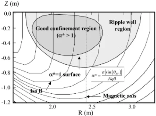
3.1 Domain in configuration space where magnetic ripple well takes place for Tore Supra tokamak . . . 70
3.2 Directions of incident electron and emitted photon with respect to the local magnetic field direction . . . 74
5.1 Grid definition for the momentum dynamics . . . 124
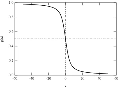
5.2 Chang and Cooper weightingfunction . . . 150
5.3 Lower Hybrid boundary problem . . . 204
5.4 Trapped domain and related flux connections . . . 207
5.5 Momentum flux connections for grid point 1 in the trapped region . . . 208
5.6 Momentum flux connections for grid point 4 in the counter-passing region . 209 5.7 Heuristic magnetic ripple modeling. The trapped/supertrapped boundary varies as well as the collision detrapping threshold are both functions of the radial location . . . 211
5.8 Trapping and detrapping process induced by radial transport . . . 215
5.9 Trapped domain for the first order distribution g . . . 219
6.1 Qualitative shape of matrix bB for the Fokker-Planck equation . . . 231
6.2 Qualitative shape of matrix bG for the drift kinetic equation . . . 233
6.3 Typical arrangement of non-zero matrix coefficients in the first 2000 columns and rows in matrix bN corresponding to the Fokker-Planck equation . . . 235
6.4 Values of the non-zero matrix coefficients after diagonal preconditionning for matrix bN0 corresponding to the Fokker-Planck equation. Dot points correspond to pitch-angle process at constant p, while full line for slowing-down process at constant ξ0. By definition values of all coefficients on the main diagonal are one . . . 235
6.5 Matrix factorization principle. Dashed areas correspond to non-zero coeffi-cients. . . 236
6.6 Reduction of the non-zero elements for the bL and bU matrices, by increasing δlu. Values of δlu are indicated on the top of each subfigure. For δlu= 10−2,
the inversion becomes instable. . . 238
6.7 Memory storage requirement reduction by increasing the δluparameter, for the Lower Hybrid current drive problem. The rate of convergence towards the steady state solution is given, using the biconjugate gradients stabilized method to solve the system of linear equations. Here only a local analysis is considered at a given radial position . . . 239
7.1 Normalized Ohmic resistivity as function of the inverse aspect ratio ² . . . . 257
7.2 Contour plot of the electron distribution function at ² = 0.31623 . . . 259
7.3 Contour plot of the stream lines at ² = 0.31623 . . . 259
7.4 Electron distribution function averaged over the perpendicular momentum direction at ² = 0.31623. Parallel and perpendicular temperatures of the electron distribution function are also shown . . . 260
7.5 Normalized Ohmic runaway rate as function of the inverse aspect ratio ² . . 261
7.6 Variations of the Lower Hybrid current and power densities, ratio between the RF and collision absorbed power density, and the current drive effi-ciency with the grid size. Here uniform pitch-angle and momentum grids are considered. Detailed aspect of the simulation are given in the text . . . 263
7.7 Variations of the memory storage requirement and the time elapsed for kinetic calculations with the grid size. Here uniform pitch-angle and mo-mentum grids are considered. Detailed aspect of the simulation are given in the text . . . 264
7.8 Variation of the current drive efficiency with the upper mometum limit of the integration domain . . . 265
7.9 Variation of the current drive efficiency with the main ion charge in the plasma . . . 266
7.10 Variation of the current drive efficiency with the amplitude of the quasilinear diffusion coefficient for the Lower Hybrid current drive problem . . . 268
7.11 Contour plot of the electron distribution function for DLH = 10 . . . 268
7.12 Contour plot of the electron distribution function for DLH = 2 . . . 269
7.13 Contour plot of the electron stream function for DLH = 2 . . . 269
7.14 Contour plot of the electron distribution function at ² = 0.31623 . . . 271
7.15 Contour plot of the Lower Hybrid quasilinear diffusion coefficient at ² = 0.31623 . . . 272
7.16 Electron distribution function averaged over the perpendicular momentum direction at ² = 0.31623. The perpendicular and parallel temperatures are also shown . . . 272
7.17 ECCD in DIII-D (ρ = 0.1, DEC = 0.15, Nk = 0.3, Y = 0.98). Output density (a), normalized current density (b), normalized absorbed power density (c), normalized current drive efficiency (d), ratio of power absorbed to power lost on collisions (e), as a function of grid size (np= nξ). . . 274
7.18 ECCD in DIII-D (ρ = 0.1, DEC = 0.15, Nk = 0.3, Y = 0.98). Output density (a), normalized current density (b), normalized absorbed power density (c), normalized current drive efficiency (d), ratio of power absorbed to power lost on collisions (e), as a function of momentum grid limit pmax
(np= 10pmax, nξ= 100). . . 276 7.19 ECCD in DIII-D (DEC = 0.15, Nk = 0.3, Y = 0.98). Output density
(a), normalized current density (b), normalized absorbed power density (c), normalized current drive efficiency (d), ratio of power absorbed to power lost on collisions (e), as a function of the inverse aspect ratio ² = r/Rp; temperatures, densities and Zeff are kept constant across the plasma. . . 277 7.20 ECCD in DIII-D (ρ = 0.1, DEC= 0.15, Nk = 0.3, Y = 0.98). 2D electron
distribution function (a), parallel distribution function (b) and perpendicu-lar temperature (c); blue thin lines represent finit, red thick lines represent f0, and green dashed contours represent DEC. . . 279
7.21 ECCD in DIII-D (θb = 0, PEC = 1 MW, Nk = 0.3, fEC = 110 MHz).
Current and power densities deposition profiles. 3D calculation with np = nξ = 100, nψ = 26. . . 280 7.22 Radial grid for 3-D JET current drive simulation. Circles correspond to the
normalized poloidal flux coordinate ψ, while crosses correspond to normal-ized radius ρ . . . 281 7.23 Pitch-angle grid for 3-D JET current drive simulation. . . 282 7.24 Momentum grid for 3-D JET current drive simulation. . . 282 7.25 Momentum grid step for 3-D JET current drive simulation. Circles
corre-spond to the flux grid, while stars to the distribution function half-grid . . 283 7.26 Ion and electron temperature and density profiles, and effective charge
pro-file used for calculating the JET magnetic equilibrium with HELENA. Here hydrogen and tritium densities are zero (pure deuterium plasma) . The poloidal flux coordinate ψ as function of the normalized radius ρ in the equatorial mid-plane corresponds to the magnetic equilibrium code output . 283 7.27 2 − D contour plot of the poloidal magnetic flux surfaces as calculated for
JET tokamak by the code HELENA . . . 284 7.28 Momentum dependence of the relativistic Maxwellian distribution function
at ρ ' 0.36, and relation between velocity v and momentum p. The devia-tion from the main diagonal indicates that above p = 4, relativistic effects become important . . . 285 7.29 2 − D contour plot in momentum space of the Lower Hybrid quasilinear
dif-fusion cofficient at ρ ' 0.36. The relativistic curvature of the lower bound of the resonance domain avoid intersection with the region of trapped elec-trons. The two full straight lines correspond to trapped/passing boundaries at that radial position . . . 286 7.30 On the left side, 2 − D contour plot of the radial diffusion rate at ρ ' 0.36.
The velocity threshold corresponds to a kinetic energy of 35 keV approxi-mately in the M KSA units. On the right side, the velocity dependence of D(0)ψ at ξ0 = 1 . . . 286
7.31 Relative particle conservation of the drift kinetic code for the 3 − D JET Lower Hybrid current drive simulation . . . 287 7.32 Flux surface averaged power density profiles for collision, RF and Ohmic
electric field absorption for the 3 − D JET Lower Hybrid current drive simulation. . . 288 7.33 Flux surface averaged current density profiles for the 3 − D JET Lower
Hybrid current drive simulation. . . 288 7.34 2 − D contour plot of the electron distribution function at ρ ' 0.36 for JET
Lower Hybrid current drive . . . 289 7.35 Electron distribution function averaged over the perpendicular momentum
direction at ρ ' 0.36 for JET Lower Hybrid current drive. The perpendic-ular and parallel temperatures are also shown . . . 290 7.36 2 − D contour plot of the electron distribution function at ρ ' 0.78 for JET
Lower Hybrid current drive . . . 290 7.37 Electron distribution function averaged over the perpendicular momentum
direction at ρ ' 0.78 for JET Lower Hybrid current drive. The perpendic-ular and parallel temperatures are also shown . . . 291 7.38 Ion and electron temperature and density profiles, and effective charge
pro-file used for calculating the Tore Supra magnetic equilibrium with HE-LENA. Here hydrogen and tritium densities are zero (pure deuterium plasma) . The poloidal flux coordinate ψ as function of the normalized radius ρ in the equatorial mid-plane corresponds to the magnetic equilibrium code output292 7.39 2 − D contour plot of the poloidal magnetic flux surfaces as calculated for
Tore Supra tokamak by the code HELENA . . . 292 7.40 Flux surface averaged current density profiles for the 3 − D Tore Supra
Lower Hybrid current drive simulation. . . 293 7.41 Magnetic ripple loss rate profile for Tore Supra tokamak in Lower
Hybrid-current drive regime, as calculated by two different methods (see the text for more details) . . . 293 7.42 2 − D contour plot of the electron distribution function at ρ ' 0.44 for Tore
Supra Lower Hybrid current drive . . . 294 7.43 Electron distribution function averaged over the perpendicular momentum
direction at ρ ' 0.44 for Tore Supra Lower Hybrid current drive. The perpendicular and parallel temperatures are also shown . . . 295 7.44 Bootstrap current profile given in the Lorentz model limit by the drift
ki-netic code and different analytical formulaes . . . 298 7.45 Effective trapped fraction as given by the by the drift kinetic code in the
Lorentz limit and by coefficient L31from analytical expression (see the text
for more details) . . . 298 7.46 Exact trapped fraction as given by the by the drift kinetic code in the
Lorentz limit and by analytical expression (see the text for more details) . . 299 7.47 Pitch-angle dependence of ef(0) and g(0)at ρ ' 0.4354 , as given by the drift
7.48 First order distribution Fk(1)0 averaged over the perpendicular momentum direction p⊥ as fonction of pk at ρ ' 0.4354 , as given by the drift kinetic code and analytical expressions, for the Lorentz model limit . . . 300 7.49 Contour plot of ef(0) at ρ ' 0.4354 , as given by the drift kinetic code for
the Lorentz model limit . . . 301 7.50 Contour plot of g(0) at ρ ' 0.4354 , as given by the drift kinetic code for
the Lorentz model limit . . . 301 7.51 Bootstrap current profile given by the drift kinetic code for the Tore Supra
magnetic configuration and different corresponding analytical formulas (see the text for more details) . . . 302 7.52 Effective trapped fraction as given by the by the drift kinetic code and the
HELENA magnetic equilbrium code for the tokamak Tore Supra . . . 302 7.53 Exact trapped fraction as given by the by the drift kinetic code for the
tokamak Tore Supra . . . 303 7.54 Pitch-angle dependence of ef(0) and g(0)at ρ ' 0.4354 , as given by the drift
kinetic code for the tokamak Tore Supra . . . 303 7.55 First order distribution Fk(1)0 averaged over the perpendicular momentum
direction p⊥ as fonction of pk at ρ ' 0.4354 , as given by the drift kinetic code for the tokamak Tore Supra . . . 304 7.56 Contour plot of ef(0) at ρ ' 0.4354 , as given by the drift kinetic code for
the tokamak Tore Supra . . . 304 7.57 Contour plot of g(0) at ρ ' 0.4354 , as given by the drift kinetic code for
the tokamak Tore Supra . . . 305 B.1 Bounce averaging coefficient λ . . . 339 C.1 Bootstrap current coefficient κ as a function of the highest terms M and N
kept in the series. . . 347 C.2 Bootstrap current coefficient κ as a function of the highest terms M and N
7.1 Ohmic conductivity as function of the e-e collision model . . . 256 7.2 Ohmic conductivity as function of the effective charge using the linearized
e-e collision model . . . 256 7.3 Runaway rate as function of the effective charge using the Maxwellian e-e
collision model . . . 258 7.4 Lower Hybrid current drive efficiencies ηLH in a pure hydrogen plasma from
various 2 − D relativistic Fokker-Planck codes . . . 267 7.5 Lower Hybrid current drive efficiencies (A · m/W ) in a pure hydrogen plasma
Introduction
The determination of the electron distribution function has a crucial importance in the tokamak plasma physics, since the toroidal current density profile that is mainly driven by electrons is intimately linked to the magnetic equilibrium and confinement performances [1]. Therefore, accurate and realistic calculations must be carried out, with the additional requirement of an optimized numerical approach, in order to reduce as much as possible both memory storage and computer time consumptions. The latter point is especially important, since kinetic calculations must be incorporated in a chain of codes for self-consistent determination of all plasma properties [2].
In this document, an extensive presentation of the fast solver for the linearized elec-tron drift kinetic is presented. This is a completely new tool based on previous numerical developments [3], that is designed for realistic calculations of the electron distribution function in the plasma region where the weak collision banana regime holds. It incorpo-rates the major physical ingredients that must be taken into account for describing the corresponding physics in a fusion reactor, namely relativistic corrections, trapped particle effects, arbitrary magnetic equilibrium for high βp regimes. For this purpose, both zero and first order kinetic equations with respect to the small drift approximation are solved, which allows to determine self-consistently boostrap current with any type of external current source (RF, Ohmic,...) at any point of the momentum space, and not only at the trapped-passing boundary as done in a previous attempt [4]. Basically, the code gives access to the neoclassical physics dominated by collisions between charged particles, for non-Maxwellian electron distribution functions. Therefore, it is particularly well suited for accurate current drive estimates in advanced tokamak regimes, including ITER, where locally, bootstrap current may strongly interplay with external current sources (ITB, edge pedestal in H-mode. . . )
Besides these physical properties, the code offer also the possibility to incorporate any type of fast electron radial transport (collision, turbulence or wave induced), which may be a key ingredient for the local control of plasma properties [5]. Written in a fully con-servative form, the code naturally conserve the electron density, but also momentum for the current drive problem, keeping first order term of the Legendre polynomial expansion of the Beliaev-Budker collision operator [6]. As usual, several useful moments of the elec-tron distribution function are calculated, namely the current density, the absorbed power, the fraction of trapped electrons, the magnetic ripple losses [7] and the bremsstrahlung
emission [8].
Advanced numerical techniques have been used, so that memory storage requirement can be strongly reduced, while keeping fast convergence rate. For this purpose the elec-tron Drift Kinetic equation is solved by the standard finite difference technique, which has proven so far to be the fastest numerical approach among all possible alternative tech-niques. Furthermore, this method is particularly well suited when large discontinuities of the diffusion or convection rates have to be considered, a case that occurs frequently when kinetic and ray-tracing calculations are coupled.
Since in most cases, the steady-state solution is seeked with respect to the largest time scale (collision or fast electron radial transport)1, the appropriate technique is the well
known upwind time differencing, corresponding to the fully implicit time scheme, whose characteristic is to be almost unconditionally stable with respect to the time step value ∆t. Nevertheless, the code offers also the possibility to investigate time dependent problems, with the usual Crank-Nicholson time differencing, which enables accurate time evolution. The bounce-averaged Drift Kinetic equation is basically a 3 − D problem, 2 − D in momentum space (slowing down, pitch-angle) et 1 − D in configuration space (radial dimension). Up to now, in order to reduce memory storage requirements, the numerical time scheme was based on the operator splitting technique, where both momentum and spatial dynamics evolved separately. If this approach turns out to be very fruitful, it has the drawback to slow down considerably the convergence towards the steady state solution, since only small time steps may be used for numericaly stable convergence. Therefore, the advantage to use fully implicit time scheme for each sub-space in hindered by this strong limitation, especially when radial transport of fast electrons must be taken into account. In order to avoid this problem, a fully implicit time scheme is considered, where both momentum and spatial dynamics are simultaneaously considered, so that no limitation occurs on the time step, which may be several order of magnitude larger than the collision reference time. However, this method requires a new technique for matrix inversion, in order to keep memory storage at an acceptable level. Indeed, with usual mesh sizes, the standard LU matrix factorization techniques does not hold anymore since matrices requirement may reach several giga-Bytes. An alternative approach is therefore absolutely necessary.
This critical point has been addressed by using advanced inversion techniques, based on incomplete LU factorization with drop tolerance. Since most of the off-diagonal coefficients of the matrices L and U are very small, one may take advantage to remove them so that the sparsity of the matrices can be greatly enhanced. Memory storage requirements can be therefore reduced drastically by one or two orders of magnitude with this pruning method, depending upon the initial matrix preconditioning, while only coefficients that are relevant of the physics problem here addressed are kept. Furthermore, computer time consumption can be also reduced, since the number of non-zero coefficients is considerably reduced. This method is similar to the strongly implicit method used for factorizing nine diagonal matrices [9], except that in this case, no restriction takes place regarding the number of diagonals. However, to take full benefit of this approach, the non-zero elements 1The energy transport time scale is usually on order on magnitude larger than the largest characteristic
time for current drive calculations, except in tokamaks of small size, where time ordering here considered in the model must be likely revisited
of the matrix which is inverted must lie predominantly along diagonals. Therefore, it may be applied for solving the zero and first order bounce-averaged Fokker-Planck equations, whose structures are well suited for this purpose, though coefficients arrangement can be complex, owing to the radial dependence of the internal trapped-passing boundary in momentum space, especialy when transport in configuration space has to be considered.
This approach has been very successfuly implemented for the electron Drift Kinetic problem in tokamaks, using the MatLab language, which provides a built-in function for incomplete LU factorization with drop tolerance, and several very efficient iterative inversion tools, like the Conjugate Gradient Squared method for solving the system of linear equations. It is important to recall that this method is also available in FORTRAN programming language2, under the package name SPARSEKIT that has also parallel
pro-cessing capabilities [10]. Moreover, the very compact MatLab programming syntax allows to design the code structure in an original way, using multidimensional objects that de-scribe simultaneously momentum and configuration space dynamics, but also wave-particle interaction. This makes the code particularly robust and easy to maintain.
In the document, the physics and numerics issues of the code are detailed, and an extensive discussion of the underlying assumptions is presented. A specific attention is paid to derive matrix coefficients in a fully consistent manner, a crucial issue especially for an accurate and robust estimate of the current drive efficiency for the various methods used in tokamaks. Some examples are shown to illustrate code performances, though still numerous possibilities remain to be investigated but are beyond the purpose of this document.
Aside from present day code capabilities, it is important to notice that the new nu-merical approach, here used, gives access to new physics domains that have never been studied accurately like wave-induce radial transport [11]. Furthermore, since the algorithm used is fast and stable, possible extensions to 4 − D problems may be foreseen like in the plateau collision regime (current drive at the very plasma edge), as well as studies of the difficult problem of electrons that are locally trapped at different spatial positions, like in stellarator. In addition the code may be extended quite in a straightforward manner to the multi-species problem, taking into account for example of the non-linear damping of the α-particles produced by fusion reactions on the electron population. However, the ion physics requires to perform orbit-averaging instead of bounce-averaging, because of the large banana width of some particles, a challenging issue for kinetic solver based on a finite difference technique. Such a requirement is crucial for describing torque induced by waves. Nevertheless, beside this difficulty, the code is already fully designed to take benefit from parallel processing, if the dynamics of various species must be studied. In particular, non-uniform momentum and pitch-angle grids are already implemented, so that refined calculations can be performed for the ions at low velocity, while accurate ones up to relativistic energies may be considered for the electrons.
2Useful informations are available on the website of Pr. Yousef Saad at the following internet address
Tokamak geometry and particle
dynamic
2.1
Coordinate system
General and specific properties of curvilinear coordinate systems are detailed in Appendix A. In this work, vectors are written in bold characters, like v, except unit vectors, which are covered with a hat, like bv.
2.1.1 Momentum Space
Because we consider gyro-averaged kinetic equations, it is important to use coordinates with rotational symmetry in order to reduce the dimensionality of the problem. Two different momentum space coordinates system are considered here:
• First, the cylindrical coordinate system¡pk, p⊥, ϕ ¢
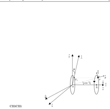
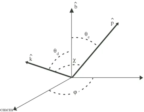
, where pk is the component of the momentum along the magnetic field, and p⊥ is the component perpendicular and ϕ is the gyro-angle. This system is defined in (A.212) and shown in Fig. 2.1. The cylindrical coordinate system is the natural system for wave-particle interaction, or also the effect of the electric field.
• Second, the spherical coordinate system (p, ξ, ϕ), where pis the magnitude of the momentum, and ξ is the cosine of the pitch-angle. This system is defined in (A.247) and shown in Fig. 2.1 as well. The spherical coordinate system is the natural system for collisions. It is the primary system, used in the Drift Kinetic code, for an accurate description of collisions.
2.1.2 Configuration Space
The particular toroidal geometry of tokamaks requires to use specific coordinates, in order to make use of symmetry properties such as axisymmetry, and takes into account the flux-surface magnetic configuration. Three different configuration space coordinates systems are considered here:
cmcm b p || ⊥ ξ O cos–1ξ p p|| ϕ p⊥ ϕ x y z
Figure 2.1: Coordinates systems ¡pk, p⊥, ϕ ¢
and (p, ξ, ϕ)for momentum dynamics
• First, the toroidal coordinate system (R, Z, φ), where R is the distance from the axis of the torus, and Z the distance along this axis . This coordinates system and the corresponding local orthogonal basis vectors
³ b R, bZ, bφ
´
are defined in (A.61) and shown in Fig. 2.2. This coordinate system conserves the largest generality in the magnetic geometry.
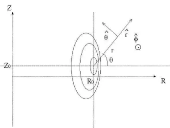
• Second, the poloidal (polar) coordinate system (r, θ, φ) assumes the existence of a toroidal axis at constant position (Rp, Zp) which is typically the plasma magnetic axis, corresponding to the position of an extremum of the poloidal magnetic flux ψ (which can be arbitrarily chosen as ψ = 0). This coordinates system and the corresponding local orthogonal basis vectors
³ b r, bθ, bφ
´
are defined in (A.94) and shown in Fig. 2.3.
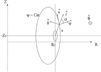
• Third, the flux coordinate system (ψ, s, φ) is the natural system when we describe particles which are confined to a given flux surface ψ. This coordinates system and the corresponding local orthogonal basis vectors
³ b ψ, bs, bφ
´
are defined in (A.136) and shown in Fig. 2.4. The vector bψ is perpendicular to the flux surface, while bs is parallel to the surface, and included in the poloidal plane. The distance s is the length along the poloidal magnetic field lines. We can choose its origin as being at the position of minimum B-field amplitude within a flux-surface.
B (ψ, s ≡ 0) = min
s {B (ψ, s)} = B0(ψ) (2.1)
Note that from now on, and all along this paper, the subscript 0 refers to quantities evaluated at the position of minimum B-field on a given flux-surface. The direction
cmcm
Figure 2.2: Coordinates system (R, Z, φ).
cmcm
cmcm
Figure 2.4: Coordinates system (ψ, s, φ).
of evolution of s is counter-clockwise and the limits smin(ψ) and smax(ψ) are set at
the position of maximum magnetic field
B (ψ, s ≡ smin) = B (ψ, s ≡ smax) = max {B (ψ, s)} = Bmax(ψ) (2.2)
• The system (ψ, θ, φ) is an alternative to the previous system, which is used to im-plement numerically the calculation of the bounce coefficients. One advantage is that the θ grid is now independent of ψ, which simplifies the numerical calcula-tions. On the other hand, the contravariant vectors ∇ψ and ∇θ are not orthogonal, and therefore are not respectively colinear with the covariant vectors ∂X/∂ψ and ∂X/∂θ. The properties of this curvilinear system are detailed in Appendix A. We also define, for geometrical purposes, a flux-function ρ (ψ) which coincides with the normalized radius on the horizontal Low Field Side (LFS) mid-plane. Indeed, in an axisymmetric system, using the functions R (ψ, θ) and Z (ψ, θ), we define ρ (ψ) as
ρ (ψ) = R (ψ, 0) − Rp
Rmax− Rp (2.3)
with 0 ≤ ρ ≤ 1 by construction, and where Rmax = R (ψmax, 0) is the value of
R on the separatrix as it crosses the mid-plane. Here ap = Rmax− Rp is defined arbitrarily as the plasma minor radius since this definition merges with the exact one for circular concentric flux-surfaces. The 2 − D outputs from the axisymmetric equilibrium code HELENA are given on the (ψ, θ) grid [12]. The system (ψ, θ, φ) will be used from now on.
cmcm b s φ v|| vs cos–1BP B
Figure 2.5: Guiding center velocity definition
2.2
Particle motion
2.2.1 Arbitrary configurationTransit or Bounce Time
Normalized Expression The transit, or bounce time, is defined as the time for a passing particle to complete a full orbit in the poloidal plane, and for a trapped particle to complete half a bounce period. Note that this is possible only in the approximation of zero banana width. Otherwise, the bounce motion would be no longer symmetric in the forth and back motions, and both would need to be accounted for. We define then
τb(ψ) = Z smax smin ds |vs| = Z smax smin ds ¯ ¯vk¯¯ B BP (2.4)
where vs is the guiding center velocity along the poloidal field lines, and vk is its velocity parallel to the magnetic field. B is the magnitude of the magnetic field, while BP is the magnitude of its poloidal component as shown in Fig. 2.5. The limits smin and smax are
defined in (2.2) for passing electrons, and are the positions, along the field lines, of turning points for trapped electrons.
The differential arc length ds along the poloidal field line is generally expressed in curvilinear coordinates ¡u1, u2, u3¢as (A.13)
ds = q
gijduiduj (2.5)
where the gij are the metric coefficients, defined in (A.12). In the (ψ, θ, φ) coordinates, the variations dψ and dφ are essentially zero along the poloidal field line. As a consequence, (2.5) becomes
The velocity and momentum are related through the relativistic factor γ (p) introduced in Sec. 6.3.3, and therefore, we have
vk v '
pk
p = ξ (2.7)
in the weak relativistic regime of tokamak plasmas, where the pitch-angle cosine ξ is defined in (A.247) We get τb(ψ) = v |ξ2π 0| Z θmax θmin dθ 2π √ g22ξξ0BB P (2.8)
where ξ0 is the pitch angle cosine at the position θ0 of minimum B-field
θ0 ≡ θ (B = B0(ψ)) (2.9)
and the limits θmin and θmax will be calculated in the next subsection.
The bounce time can be normalized as such: τb(ψ, ξ0) = 2πRv |ξpeq (ψ) 0| λ (ψ, ξ0) (2.10) with λ (ψ, ξ0) = eq (ψ)1 Z θmax θmin dθ 2π √ g22 Rp ξ0 ξ B BP (2.11) and e q (ψ) ≡ Z 2π 0 dθ 2π √ g22 Rp B BP (2.12)
The bounce time is normalized to the transit time of particles with parallel momentum only, such that λ (ψ, ±1) = 1.
The covariant metric element g22 is given by (A.10)-(A.12), which is in the (ψ, θ, φ) system becomes (A.192)
g22= |J∇ψ × ∇φ|2= ¯¯ r ¯ bψ · br ¯ ¯ ¯ (2.13) Consequently, the normalized bounce time takes the form
λ (ψ, ξ0) = eq (ψ)1 Z θmax θmin dθ 2π 1 ¯ ¯ ¯ bψ · br ¯ ¯ ¯ r Rp B BP ξ0 ξ (2.14) with e q (ψ) = Z 2π 0 dθ 2π 1 ¯ ¯ ¯ bψ · br ¯ ¯ ¯ r Rp B BP (2.15)
Particle Motion in the Magnetic Field The particle motion along the magnetic field lines exhibits one constant of the motion, the energy (or the total momentum p), and an adiabatic invariant, the magnetic moment µ. They are given by the equations
p2= p2⊥+ p2k (2.16)
µ = p
2
⊥
2meB (2.17)
such that, as a function of the moment component¡pk0, p⊥0 ¢
at the location θ0of minimum
B-field, we have p2⊥+ p2k = p2⊥0+ p2k0 (2.18) p2 ⊥ B (ψ, θ) = p2 ⊥0 B0(ψ) (2.19) Using the transformation (A.250-A.251) from¡pk, p⊥
¢ to (p, ξ), the system (2.18-2.19) becomes p2= p20 (2.20) 1 − ξ2 B (ψ, θ) = 1 − ξ2 0 B0(ψ) (2.21) We get an expression for ξ as a function of ξ0:
ξ (ψ, θ, ξ0) = σ q 1 − Ψ (ψ, θ)¡1 − ξ2 0 ¢ (2.22) where σ = sign (ξ0) = sign
¡
vk¢, and Ψ (ψ, θ) is the ratio of the total magnetic field B to its minimum value B0
Ψ (ψ, θ) ≡ B (ψ, θ)
B0(ψ) (2.23)
The trapping condition is given by |ξ0| < ξ0T(ψ) , where ξ0T(ψ) is the pitch angle,
defined at the minimum B0(ψ) on a given flux-surface, such that the parallel velocity of
the particle vanishes at the maximum Bmax(ψ). An expression for ξ0T(ψ) can then be
obtained from (2.22): setting ξ (ξ0T, B = Bmax(ψ)) = 0, we get
ξ20T(ψ) = 1 − B0(ψ)
Bmax(ψ) (2.24)
The turning points are
θmin(ψ, ξ0) =
¯ ¯ ¯
¯ θT min−π for trapped particlesfor passing particles (2.25) θmax(ψ, ξ0) =
¯ ¯ ¯
We can determine the turning angles θT min(ψ, ξ0) and θT max(ψ, ξ0) as the position
where ξ (ψ, θ, ξ0) = 0. At this position, we have B = Bb(ψ, ξ0), where Bb(ψ, ξ0) is then
given by (2.22) Bb(ψ, ξ0) = B0(ψ) 1 − ξ2 0 (2.27) so that θT min(ψ, ξ0) = θ (B = Bb|θ < θ0) [2π] (2.28) θT max(ψ, ξ0) = θ (B = Bb|θ > θ0) [2π] (2.29) where θ0 is given by (2.9).
Calculation of λ (ψ, ξ0) From the Output Data of Equilibrium Codes The nu-merical calculation of λ (ψ, ξ0) can be carried from the output of any magnetic equilibrium
code. In the kinetic code here considered, we use HELENA for magnetic flux surface cal-culations [12], since it is used in the the CRONOS tokamak simulation package [2].
Data are assumed to be the parametrization of the flux-surfaces R (ψ, θ) and Z (ψ, θ), and the three components of the magnetic field BR(ψ, θ), BZ(ψ, θ) and Bφ(ψ, θ). From these components we derive directly the toroidal and poloidal components of the field, as well as the total field:
BT(ψ, θ) = |Bφ(ψ, θ)| BP(ψ, θ) = q B2 R(ψ, θ) + BZ2 (ψ, θ) B (ψ, θ) = q B2 T (ψ, θ) + BP2 (ψ, θ) (2.30) and also Rp = R (0, θ) (2.31) Zp = Z (0, θ) (2.32)
We also have an expression for r r (ψ, θ) =
q
(R (ψ, θ) − Rp)2+ (Z (ψ, θ) − Zp)2 (2.33) and, using relation
b r = ³ b r · bR ´ b R + ³ b r · bZ ´ b Z = µ R (ψ, θ) − Rp r ¶ b R + µ Z (ψ, θ) − Zp r ¶ b Z (2.34)
that can be easily deduced from vector relation in Fig. 2.2, we get an expression for the scalar product b ψ · br = ³ ∇ψ · bR ´ (R (ψ, θ) − Rp) + ³ ∇ψ · bZ ´ (Z (ψ, θ) − Zp) r |∇ψ| (2.35)
In a toroidal axisymmetric geometry, the magnetic field can be expressed generally as B = I (ψ) ∇φ + ∇ψ × ∇φ (2.36) so that BT = |I (ψ)| |∇φ| = |I (ψ)| R (2.37) BP = |∇ψ| |∇φ| = |∇ψ|R (2.38) We also have BT = I (ψ) ∇φ = Bφφb (2.39) BP = ∇ψ × ∇φ = −BPbs (2.40) and therefore ∇φ × BP = ∇φ × (∇ψ × ∇φ) = |∇φ|2∇ψ (2.41) so that ∇ψ = ∇φ × BP |∇φ|2 = R bφ × BP (2.42)
and we have the projections ³ ∇ψ · bR ´ = R bR · bφ × BP = −RBZ (2.43) ³ ∇ψ · bZ ´ = R bZ · bφ × BP = RBR (2.44)
Finally, the expressions for the normalized bounce time λ and eq that are used in numerical calculations are
λ (ψ, ξ0) = q (ψ)e1 Z θmax θmin dθ 2π B h (R − Rp)2+ (Z − Zp)2 i Rp|BR(Z − Zp) − BZ(R − Rp)| ξ0 ξ (2.45) with e q (ψ) = Z 2π 0 dθ 2π B h (R − Rp)2+ (Z − Zp)2 i Rp|BR(Z − Zp) − BZ(R − Rp)| (2.46) where R, Z, BR, BZ and B are functions of (ψ, θ), and ξ is a function of (ψ, θ, ξ0) given by
(2.22).
Safety Factor q (ψ) The (averaged) safety factor q is defined in Ref. [13] in a general way as q (ψ) = I (ψ) 4π2 δV δψ R−2® (2.47)
It can be expressed as q (ψ) = I (ψ) Z 2π 0 dθ 2π Z 2π 0 dφ 2π J R2 (2.48)
where the Jacobian J is given by (A.195)
J = |∇ψ × ∇θ · ∇φ|−1 = Rr |∇ψ| ¯ ¯ ¯ bψ · br ¯ ¯ ¯ = r BP 1 ¯ ¯ ¯ bψ · br ¯ ¯ ¯ (2.49) where (2.40) is used We obtain q (ψ) = I (ψ) Z 2π 0 dθ 2π 1 ¯ ¯ ¯ bψ · br ¯ ¯ ¯ r BPR2 (2.50) and, using (2.36), we finally have
q (ψ) = Z 2π 0 dθ 2π 1 ¯ ¯ ¯ bψ · br ¯ ¯ ¯ r R BT BP (2.51)
The expression of q (ψ) and its relation to eq (ψ) in the simplified case of circular con-centric flux-surfaces will be addressed in sub-section 2.2.2.
Using (2.33) and (2.35), we find the expression
q (ψ) = Z 2π 0 dθ 2π h (R − Rp)2+ (Z − Zp)2 i BT R |BR(Z − Zp) − BZ(R − Rp)| (2.52) that is convenient for the numerical evaluation.
Toroidal Extent of Banana Orbits
We are interested in calculating the toroidal extent of banana orbits, that is, the toroidal angle corresponding to the path done by a trapped particle between two turning points. It is given by
∆φ = φmax− φmin=
Z φmax φmin
dφ (2.53)
and can be expressed as a function of the length element dl along the path, using (A.198) ∆φ = Z l(φmax) l(φmin) dl (φ) dφ dl (φ) = Z l(φmax) l(φmin) dl (φ) R (2.54)
The poloidal and toroidal elements are related through the local angle of the magnetic field, dl (φ) dl (θ) = BT BP (2.55) so that ∆φ = Z l(φmax) l(φmin) dl (φ) dφ dl (φ) = Z l(θmax) l(θmin) 1 R BT BPdl (θ) (2.56)
Using (A.197), we get
∆φ = Z θmax θmin dθ ¯¯ 1 ¯ bψ · br ¯ ¯ ¯ r R BT BP (2.57) Defining the integral
qT (ψ, ξ0) = Z θmax θmin dθ 2π 1 ¯ ¯ ¯ bψ · br ¯ ¯ ¯ r R BT BP (2.58)
we find that the toroidal extent of banana orbits is ∆φ
2π = qT (ψ, ξ0) (2.59)
Note that at the trapped/passing limit, we have lim
ξ0→ξ0T ∆φ
2π = qT (ψ, ξ0T) = q (ψ) (2.60)
Therefore, we retrieve the interpretation of the safety factors, which is the number of toroidal rotations ∆φ/2π for one poloidal rotation.
Bounce Average
In order to reduce the dimension of kinetic equations, it is important to define an average over the poloidal motion, which anihilates the term that accounts for the time evolution of the variations of the distribution function along the field lines. The natural average is
{A} = 1 τb " 1 2 X σ # T Z smax smin ds |vs|A (2.61)
where the sum over σ applies to trapped particles only.
It can be rewritten in terms of the normalized bounce time λ using expression (2.11) {A} = 1 λeq " 1 2 X σ # T Z θmax θmin dθ 2π √ g22 Rp B BP ξ0 ξ A (2.62) or {A} = 1 λeq " 1 2 X σ # T Z θmax θmin dθ 2π 1 ¯ ¯ ¯ bψ · br ¯ ¯ ¯ r Rp B BP ξ0 ξ A (2.63)
using relation (2.13).
Another expression uses the output data from equilibrium codes. Following the work in the previous section, we find
{A} = 1 λeq " 1 2 X σ # T Z θmax θmin dθ 2π B h (R − Rp)2+ (Z − Zp)2 i Rp|BR(Z − Zp) − BZ(R − Rp)| ξ0 ξ A (2.64) or explicitely {A} = Z θmax θmin dθ 2π B h (R − Rp)2+ (Z − Zp)2 i Rp|BR(Z − Zp) − BZ(R − Rp)| ξ0 ξ −1 × " 1 2 X σ # T Z θmax θmin dθ 2π B h (R − Rp)2+ (Z − Zp)2 i Rp|BR(Z − Zp) − BZ(R − Rp)| ξ0 ξ A (2.65)
The bounce averaging of momentum-space operators in the kinetic equations leads to a set of coefficients that all have a similar structure, denoted λk,l,m and λk,l,m, which are
define as (µ ξ (ψ, θ, ξ0) ξ0 ¶k Ψl(ψ, θ) µ R0(ψ) R (ψ, θ) ¶m) = λk,l,m(ψ, ξ0) λ (ψ, ξ0) (2.66) and σ ( σ µ ξ (ψ, θ, ξ0) ξ0 ¶k Ψl(ψ, θ) µ R0(ψ) R (ψ, θ) ¶m) = λk,l,m(ψ, ξ0) λ (ψ, ξ0) (2.67) where R0(ψ) ≡ R (ψ, θ0) (2.68)
Note that by definition, λ0,0,0 = λ. In addition,
λk,l,m= ¯ ¯ ¯
¯ λ0k,l,m for passing particlesfor trapped particles (2.69)
2.2.2 Circular configuration
Parametrization of the Flux-Surfaces
In this case, we have ψ = ψ (r) and therefore it is easier to work in the (r, θ, φ) coordinate to account for the symmetry in the problem. The normalized radius is
ρ (ψ) = r ap (2.70) We have now b ψ = br (2.71) so that (A.113) √ g22= r (2.72)
Magnetic Field The toroidal field is
BT(r, θ) = |I (r)|
R (r, θ) (2.73)
and the poloidal field is
BP(r, θ) = |∇ψ (r)|R (r, θ) (2.74) where |∇ψ (r)| = ¯ ¯ ¯ ¯dψ (r)dr ¯ ¯ ¯ ¯ = a1 p ¯ ¯ ¯ ¯dψ (ρ)dρ ¯ ¯ ¯ ¯ (2.75)
is now only a function of r or ρ. The total field is then
B (r, θ) = q
I2(r) + |∇ψ (r)|2
R (r, θ) (2.76)
and can be written as
B (r, θ) = B0(r)R (r, θ)R0 (2.77) with B0(r) = q I2(r) + |∇ψ (r)|2 R0 (2.78)
Consequently, we ratio of magnetic fields Ψ as defined in (2.23) becomes Ψ (r, θ) = R0 R (r, θ) (2.79) and B BP = q I2(r) + |∇ψ (r)|2 |∇ψ (r)| = s 1 + I2(r) |∇ψ (r)|2 (2.80) is a function of r only. Safety factor
The safety factor given by expression (2.51) becomes q (r) = Z 2π 0 dθ 2π r R BT BP = r Rp BT BP Z 2π 0 dθ 2π Rp R (2.81)
The averaged value of Rp/R is evaluated in (B.27). It gives Z 2π 0 dθ 2π Rp R = 1 q 1 − (r/Rp)2 (2.82)
so that q (ψ) = q 1 1 − (r/Rp)2 r Rp BT BP (2.83)
Note that in the factor q
1 − (r/Rp)2 is usually neglected, which is valid only in the large aspect ratio approximation, i.e. when the inverse aspect ratio ² defined as
² = r
Rp (2.84)
is much less than unity. Particle Motion Using relation (A.95),
R (r, θ) = Rp+ r cos θ (2.85)
and recalling that the minimum B-field B0 corresponds to the poloidal angle value in that case
θ0 = 0 (2.86)
we find
Rmin(r) = Rp− r = Rp(1 − ²) (2.87)
Rmax(r) = Rp+ r = Rp(1 + ²) = R0(r) (2.88)
Therefore, the expression (2.79) becomes
Ψ (ρ, θ) = 1 + ²
1 + ² cos θ (2.89)
and using relation (2.77)
Bmax(r) = B0(r)1 + ²1 − ² (2.90)
expression (2.24) is
ξ0T2 (r) = 2²
1 + ² (2.91)
The pitch-angle cosine ξ is then given by combining relations (2.22 ) and (2.89) ξ (r, θ, ξ0) = σ r 1 − 1 + ² 1 + ² cos θ ¡ 1 − ξ2 0 ¢ (2.92) and the the turning angles are obtained from expression (2.27), or in the present notation
B (r, θT) = Bb(r, ξ0) = B1 − ξ0(r)2 0
(2.93) Using relation (2.89), one obtains
B0(r) 1 + ² 1 + ² cos θT = B0(r) 1 − ξ2 0 (2.94)
and then ξ02 = 1 −1 + ² cos θT 1 + ² = ² (1 − cos θT) 1 + ² (2.95) so that θT = arccos · 1 −2ξ02 ξ2 0T ¸ (2.96) and finally by symmetry
θT min= −θT (2.97)
θT max= θT Bounce Time
Using (2.72), the normalized bounce time reduces to λ (r, ξ0) = q²e Z θmax θmin dθ 2π ξ0 ξ B BP (2.98)
with, using definition (2.15)
e q (r) = ² Z 2π 0 dθ 2π B BP (2.99) Because B/BP only a function of r, as seen in (2.80), and can be taken out of the integrals, we get finally
λ (r, ξ0) = Z θmax θmin dθ 2π ξ0 ξ (2.100)
This integral can be performed analytically in a series expansion whose coefficients are calculated in (B.1). Note that in the case where BT À BP and in the large aspect ratio approximation ² ¿ 1, we have eq (r) → q (r), which explains the notations, and the introduction of pseudo safety factor like eq. Other new definitions of pseudo safety factors will be introduced throughout the next sections, based on similar arguments.
Kinetic description of electrons
3.1
Boltzman equation; Gyro- and Wave-averaging
In the kinetic description, electrons are described by a distribution function f (r, p, t), which gives the density in phase space of particles with a momentum p at a position r and at time t. The particle conservation equation in phase space is the Boltzmann equation
∂f ∂t + v · ∇rf + qe[E (r, t) + v × B (r, t)] · ∇pf = ∂f ∂t ¯ ¯ ¯ ¯ C (3.1) where ∂f ∂t ¯ ¯ ¯ ¯ C ≡ C (f ) (3.2)
is the collision operator. The fields E (r, t) and B (r, t) are assumed to consist of time-independent macroscopic fields E (r) and B (r) and fields associated with plane waves.
E (r, t) = E ( r) + Z e Ekei(k·r−ωt)dk (3.3) B (r, t) = B (r) + Z e Bkei(k·r−ωt)dk (3.4)
Because we are interested in solving the kinetic equation on the bounce and collisional time scales, we need to average over the faster time scales, which are the gyromotion and the wave oscillation.
Performing a time-averagingR02π/ωdt of the equation (3.1) removes the fast wave time scale from the equation, to give
∂f ∂t + v · ∇rf + qe £ E (r) + v × B (r)¤· ∇pf = ∂f ∂t ¯ ¯ ¯ ¯ C − Z 2π/ω 0 dt X k ³ qe h e Ek+ v × eBk i · ∇pf ´ (3.5)
where
f = Z 2π/ω
0
dt f (3.6)
is the wave-period averaged distribution function. The time derivative in the first term of (3.5) implicitely refers to times longer than the wave period ω.
Under the assumption of a strong magnetic field, such that the gyrofrequency Ωe Ωe= qeB
γme
(3.7) is much larger than both the collisional frequency and the bounce frequency, we can expand the distribution function
f = f0+ f1+ f2+ · · · (3.8)
with a small parameter
δ ∼ ωb Ωe
∼ νc Ωe
(3.9) The zero order equation becomes
qev × B (r) · ∇pf0 = 0 (3.10)
We have, in the¡pk, p⊥, ϕ¢space defined in Appendix A,
v = p
γ¡pk, p⊥ ¢
me
(3.11) with the momentum being given by relation (A.214)
p = pkbk + p⊥⊥b (3.12)
and the gradient by expression (A.239) ∇pf = ∂p∂f k b k + ∂f ∂p⊥⊥ +b 1 p⊥ ∂f ∂ϕϕb (3.13)
In this system, by definition,
B (r) = B (r) bk (3.14)
so that the gyromotion operator becomes
qev × B (r) · ∇p = Ωe ³ p × bk ´ · ∇pf = −Ωe∂ϕ∂ (3.15)
The equation (3.10) becomes consequently ∂f0
and therefore f0 is independent of ϕ. The first order equation is ∂f0 ∂t + v · ∇rf 0+ qeE (r) · ∇pf0+ qev × B (r) · ∇pf1 = ∂f0 ∂t ¯ ¯ ¯ ¯ C − Z 2π/ω 0 dt X k ³ qe h e Ek+ v × eBk i · ∇pf ´ (3.17) The last term in the equation (3.17) has been calculated by Lerche for a uniform plasma, in the form of a quasilinear operator Q¡f¢. We can rewrite
C¡f0¢= ∂f0 ∂t ¯ ¯ ¯ ¯ C (3.18) Q¡f0¢= − Z 2π/ω 0 dt X k ³ qe h e Ek+ v × eBk i · ∇pf ´ (3.19) Performing the gyro-averaging R02πdϕ on the kinetic equation (3.17), we find, using (3.16), that Z 2π 0 dϕ ∂ ef0 ∂t = ∂ ef0 ∂t (3.20) and Z 2π 0 dϕ v · ∇rf0 = Z 2π 0 (dϕ v) · ∇rf0= vgc· ∇rf0 (3.21) where vgc is the electron velocity along the guiding center.
Concerning the electric field, we decompose the gradient in momentum space using (3.13) Z 2π 0 dϕ qeE (r) · ∇pf0 = qeE (r) · Z 2π 0 dϕ · ∂f0 ∂pkbk + ∂f0 ∂p⊥ b ⊥ + 1 p⊥ ∂f0 ∂ϕϕb ¸ (3.22) = qe ∂f0 ∂pkE (r) · bk +qe∂p∂f0 ⊥E (r) · Z 2π 0 dϕ b⊥ +qe p⊥ E (r) · Z 2π 0 dϕ∂f0 ∂ϕϕb (3.23) and, using Z 2π 0 dϕ b⊥ = 0 (3.24) Z 2π 0 dϕ∂f0 ∂ϕϕ = −fb 0 Z 2π 0 dϕ∂ bϕ ∂ϕ = f0 Z 2π 0 dϕ b⊥ = 0 (3.25) we obtain Z 2π 0 dϕ qeE (r) · ∇pf0 = qeEk(r) ∂f0 ∂pk (3.26)
The gyromotion term is averaged to zero Z 2π 0 dϕ qev × B (r) · ∇pf1 = −Ωe Z 2π 0 dϕ ∂f1 ∂ϕ = 0 (3.27)
so that we get finally ∂ ef0 ∂t + vgc· ∇rfe0+ qeEk ∂ ∂pk (r) ef0 = C ³ e f0 ´ + Q ³ e f0 ´ (3.28) This equation is called electron drift-kinetic equation. Renaming the guiding-center distribution function f0 = f¡r, pk, p⊥, t
¢
, E (r) = E (r) and B (r) = B (r) , we get ∂f
∂t + vgc· ∇f = C (f ) + Q (f ) + E (f ) (3.29) where we define an electric field operator
E (f ) = −qeEk(r) ∂
∂pkf (3.30)
Implicitely, the time scale here considered is so that t À (2π/ω, 2π/Ωe) .
3.2
Guiding-Center Drifts and Drift-Kinetic Equation
As shown in previous section, for axisymmetric plasmas, the electron drift kinetic equation may be expressed in the general form
∂f
∂t + vgc· ∇f = C (f ) + Q (f ) + E (f ) (3.31) where f = f (p, ξ, ψ, θ, t) is the guiding-center distribution function.
In tokamaks, it can be shown that the guiding center velocity vgcmay be decomposed
into a fast parallel motion along the field lines, and a vertical drift velocity vD across the magnetic flux surfaces
vgc= vkbb + vD (3.32)
From the general expression (2.36) of the magnetic field B,
B = I (ψ) ∇φ + ∇ψ × ∇φ (3.33)
one obtains in the (ψ, s, φ) coordinates system, B = I (ψ)
R φ −b |∇ψ|
R bs (3.34)
As shown in Appendix A, the gradient in (ψ, s, φ) coordinates is ∇ = ∇ψ ∂ ∂ψ + ∇s ∂ ∂s + ∇φ ∂ ∂φ = ∇ψ ∂ ∂ψ + bs ∂ ∂s + b φ R ∂ ∂φ (3.35)
and recalling that the constants of the motion are the total energy (or momentum p) as defined in (2.16) and the magnetic moment µ as given by relation (2.17), following conservations laws ∂µ ∂s = 0 (3.36) ∂ ∂s h p2k+ 2µBme i = 0 (3.37) are satisfied.
3.2.1 Drift Velocity from the Conservation of Canonical Momentum
The toroidal canonical momentum is also a constant of the motion because of axisymmetry. It is expressed as
Pφ= R [γmevφ+ qeAφ] (3.38)
where Aφ is the toroidal component of the vector potential. From the relation
B = ∇ × A (3.39)
and the expression (A.171) of a rotational in (ψ, s, φ) coordinates, we get B = · 1 R ∂ ∂s(RAφ) − 1 R ∂ ∂φ(As) ¸ b ψ + · 1 R ∂ ∂φ(Aψ) − |∇ψ| R ∂ ∂ψ(RAφ) ¸ b s + · |∇ψ| ∂ ∂ψ (As) − |∇ψ| ∂ ∂s µ Aψ |∇ψ| ¶¸ b φ (3.40) with Aψ = A · bψ (3.41) As = A · bs (3.42) Aφ = A · bφ (3.43)
In axisymmetric plasma, this reduces to
B = 1 R ∂ ∂s(RAφ) bψ −|∇ψ| R ∂ ∂ψ(RAφ) bs + · |∇ψ| ∂ ∂ψ (As) − |∇ψ| ∂ ∂s µ Aψ |∇ψ| ¶¸ b φ (3.44) so that Bs = −|∇ψ|R ∂ψ∂ (RAφ) (3.45)
In addition, we know from expression (3.34) that
Bs= −|∇ψ|R (3.46)
so that be obtain
∂RAφ
∂ψ = 1 (3.47)
Because the toroidal canonical momentum is a constant of the motion, we have
vgc· ∇Pφ= 0 (3.48)
which can be decomposed into
vgc· ∇ (Rγmevφ) + vgc· ∇ (qeRAφ) = 0 (3.49) Using relation (A.169), we get
vgc· ∇ (qeRAφ) = vgc· " ∇ψ ∂ ∂ψ + bs ∂ ∂s+ b φ R ∂ ∂φ # (qeRAφ) (3.50)
which in axisymmetric systems gives
vgc· ∇ (qeAφ) = qevgc· · ∇ψ∂RAφ ∂ψ + bs ∂RAφ ∂s ¸ (3.51) Since Bψ = 0, we have from relation (3.44) ∂ (RAφ) /∂s = 0 and therefore, using expression (3.47),
vgc· ∇ (qeAφ) = qevgc· ∇ψ (3.52)
The only velocity accross the flux-surfaces is the drift velocity we are looking for, so that we get, using relation (3.32)
vgc· ∇ (qeAφ) = qevD· ∇ψ (3.53) and the equation (3.49) becomes
qevD· ∇ψ = −vgc· ∇ (Rγmevφ) (3.54) Assuming a priori that¯¯vk¯¯ À |vD|, a condition that holds in tokamaks, this equation reduces to vD· ∇ψ = −q1 e vk BB · ∇ (Rγmevφ) = −vk ΩeB · ∇ (Rvφ) (3.55)
where we used that ∂γ/∂s = 0 because of the conservation of energy. The toroidal velocity is related to the parallel velocity by
vφ= Bφ B vk =
I (ψ)