Operational dependability model generation

(1)

HAL Id: tel-03177207

https://tel.archives-ouvertes.fr/tel-03177207

Submitted on 26 Mar 2021

HAL is a multi-disciplinary open access

archive for the deposit and dissemination of sci-entific research documents, whether they are pub-lished or not. The documents may come from teaching and research institutions in France or abroad, or from public or private research centers.

L’archive ouverte pluridisciplinaire HAL, est destinée au dépôt et à la diffusion de documents scientifiques de niveau recherche, publiés ou non, émanant des établissements d’enseignement et de recherche français ou étrangers, des laboratoires publics ou privés.

Changyi Xu

To cite this version:

Changyi Xu. Operational dependability model generation. Automatic. Université de Lyon, 2020. English. �NNT : 2020LYSEI129�. �tel-03177207�

(2)

THÈSE de DOCTORAT DE L’UNIVERSITÉ DE LYON

opérée au sein de

I’Institut National des Sciences Appliquées de Lyon

Ecole Doctorale

160 Électronique, Électrotechnique, Automatique

Spécialité/ discipline de doctorat :

Automatique

Soutenue publiquement le 16/12/2020, par:

Changyi XU

Operational Dependability Model Generation

Devant le jury composé de :

KOBI Abdelssamad Professeur (Université d'Angers) Rapporteur

BERRUET Pascal Professeur (Université Bretagne Sud) Rapporteur

LANUSSE Agnes Ingénieur Chercheur (CEA) Examinatrice

BRINZEI Nicolae Maître de conférences (Université de Lorraine) Examinateur

NIEL Eric Professeur (INSA Lyon) Directeur de thèse

(3)

(4)

Acknowledges

This research work was carried out between 2015 and 2020 at the Laboratory Ampere. I would like to express my heartfelt gratitude to all those whole helped me during the completion of this thesis. Without their support and encouragement, this thesis could not be finished.

First and foremost, I owe a special debt of gratitude to my supervisor, Professor Eric NIEL, for his invaluable help. He has walked me through all the stages of this PhD research and thesis writing. I really appreciate his rigorous scientific attitude and his profound accumulation of academic knowledge. His patient guidance and valuable suggestion is the wealth of my life. I also gratefully acknowledge the help of my co-supervisor, Professor Emil DUMITRESCU, who has offered me expert guidance in my academic study. He brought me a positive way of working, especially an optimistic attitude towards life. Without his great devotion of time or his insightful criticism, the completion of this thesis would not have been possible.

Second, I would give my hearty thanks to Mahya RAHIMI, Xiaoshan LU, Tahereh VAEZI, Xiaokang ZHANG, Teng ZHANG, Fei LIU and all the other faculty members in Laboratory Ampere. Their precious suggestions and valuable help in various aspects made me feel like home. Special thanks for Chao ZHANG, Lianxin HU, Lianxin’s wife Ruijuan LIU, Xiao LI, Weigang FAN, Nan ZHANG and all my friends in France. We lived together, we helped each other, and we witnessed every smile and every drop of tear. Each moment is my valuable memory.

Third, my sincere gratitude would go to my beloved family and relatives, for their selfless help and solicitude in all sorts of ways. Much indebted to my parents, they have given me my life, they educated me with their life savings, they have supported me in each stage, especially, at any cost，they are always being prepared to raise me up at every moment I am failing down. Also, here expresses the mourning for my grandparents HE&CHANG, who built a big family where members look for each other for every silver lining and every happiness, who brought me up and made my childhood joyous and carefree. As the distance returning home was too long, I could not attend my grandfather's funeral in time, which makes me regretful in the rest of my life. May the past rest in peace, the living predicament.

Last but not the least, I cherish for my motherland-China the liveliest feeling of affection and gratitude. I am grateful for China Scholarship Council for supporting my research and living in France.

(5)

(6)

Abstract

Assessing complex industrial systems to be on dependable service is what the engineers and researchers have long been aiming for. Recent advanced researches in the Model-based safety assessment, especially the Structre Analysis and Component Modeling, provide the practicable methodologies to assess the dependability, yet a lack of the framework which is able to assess both the structure and the various behaviors of the components in one uniformed model retains them to achieve the excellent assessment. Moreover, as the system’s operations are not considerable in the models, the service in the aspect of operational dependability is not able to be assessed both in quality and in quantity. Although several existing assessment tools have already show their potential to model the various behaviors in the form of n-state models or consider the operations as repair priority to be event sequence in the model, fusing ‘structure’, ‘various behaviors’ and ‘operations’ is still a challenge, highlighting a need for one viable framework that bridge the gap among them both by quality or quantity. In this research, a formal model generation approach is studied to bridge this gap, which is able to assess the system operatinal dependability by considering the system structure, various behaviors, and operations. Here, the composition of the component models is introduced in order to generate a global model of the system, the total breakdown states are identified according to the resulted failure expression for the purpose to fully consider the system’s structure, and the operational dependability is further realized by quality by applying the trajectory specifications, while by quantity by developing a cost evaluating technology termed Capacity Calculation Fault Tree. In the end, a demonstration of a miniplant system illustrates the wide potential of this research for guaranteeing the dependable service of complex industrial systems.

KEYWORDS: Model-based safety assessment, Operational dependability, Dependability model

(7)

(8)

Résumé

L'objectif à long terme des ingénieurs et des chercheurs est d'évaluer la fiabilité des systèmes industriels complexes. Les évaluations de la sécurité fondées sur des modèles effectuées ces dernières années, en particulier les études d'analyse structurelle et de modélisation des composants, fournissent des méthodes pratiques d'évaluation de la fiabilité,Toutefois, l'absence d'un cadre permettant d'évaluer simultanément la structure et les comportements des différents éléments d'un modèle unifié n'a pas permis d'obtenir d'excellentes évaluations. En outre, les opérations du système n'étant pas pris en compte dans le modèle, il n'est pas possible d'évaluer la qualité et la quantité du service en termes de fiabilité du opérations. Cette invention concerne un procédé de génération de modèle formalisé qui permet d 'évaluer la fiabilité du fonctionnement du système en tenant compte de sa structure, de ses divers comportements et de ses opérations. La composition du modèle de composant est introduite pour générer un modèle global du système. Afin de tenir pleinement compte de la structure du système, l 'état total de défaillance du système est déterminé sur la base de l' expression de défaillance obtenue. Sur le plan qualitatif, la fiabilité opérationnelle est encore renforcée par l'application des spécifications de trajectoire.Et, Sur le plan quantitif, il est renforcée par la mise au point d'une technique d'évaluation des coûts appelée arbre de calcul de capacité. Enfin, l'exemple d'un système industriel illustre l'énorme potentiel qu'offre l'étude pour garantir la fiabilité des services fournis par les systèmes industriels complexes.

MOTS CLÉS: Évaluation de la sécurité fondée sur des modèles, Fiabilité opérationnelle, Génération

(9)

(10)

List of Figures

Figure 1 Dependable systems design flow ... 7

Figure 2 RAM Markov chain model ... 9

Figure 3 system：structure and service ... 11

Figure 4 series structure system ... 13

Figure 5 Parallel structure system ... 14

Figure 6 Cold redundancy structure ... 15

Figure 7 Warm redundancy structure ... 15

Figure 8 Vote structure system ... 16

Figure 9 Series-Parallel Structure ... 17

Figure 10 Mixed Structure... 17

Figure 11 Basic reliability CTMC models from structure definitions ... 20

Figure 12 composition operation of interactive Markov chain ... 22

Figure 13 State combination ... 23

Figure 14 Interaction of Petri Net ... 25

Figure 15 Petri Net model generation based on structure and FtA... 26

Figure 16 transformation between Stochastic Petri Net and CTMC ... 28

Figure 17 BDMP ... 30

Figure 18 Overview of AltaRica 3.0 project ... 31

Figure 19 Time indicators calculation by GRIF CTMC ... 33

Figure 20 Fault tree Analysis ... 33

Figure 21 RBD assessment approach ... 34

Figure 22 Petri Net Assessment Approach for Redundancy system ... 35

Figure 23 framework of proposal ... 41

Figure 24 framework of GRA generation... 42

Figure 25 framework of operational dependability ... 43

Figure 26 Model translation between CTMC and EDA ... 46

(13)

Figure 28 TBS identification for Reliability CTMC establishment ... 52

Figure 29 Benchmark: Consideration of Higher-level Reliability ... 56

Figure 30 "G1 has the priority to repair" Model Specifying ... 59

Figure 31 Downtime Maintenance specifying approach ... 64

Figure 32 Priority to repair specifying approach ... 65

Figure 33 First failed first repaired specifying approach ... 59

Figure 34 Management specifying benchmark for DM, PtR and FFFR ... 66

Figure 35 ‘and’ gate of CCFT for parallel structure ... 68

Figure 36 ‘or’ gate of CCFT for series structure ... 69

Figure 37 power plant system ... 70

Figure 38 GRA generation with specifications ... 72

Figure 39 CCFT modeling... 73

Figure 40 System dynamic capacity simulation (without management requirement) ... 75

Figure 41 Simulation of the system production capacity with management requirement ... 75

Figure 42 Mini Plant system... 83

Figure 43 components in miniplant ... 84

Figure 44 CCFT for miniplant ... 86

Figure 45 Specification Automata based on the management requirements ... 87

Figure 46 Simulation for G2G3 ... 90

Figure 47 Simulation for G4... 90

Figure 48 Simulation for PtR4(1)(2) and PtR5(3)(4) ... 90

Figure 49 Simulation for FFFR67 ... 91

Figure 50 Simulation method of Management requirement effectiveness ... 92

Figure 51 Simulation for PtR4 ... 93

Figure 52 simulation for PtR5 ... 94

(14)

List of Tables

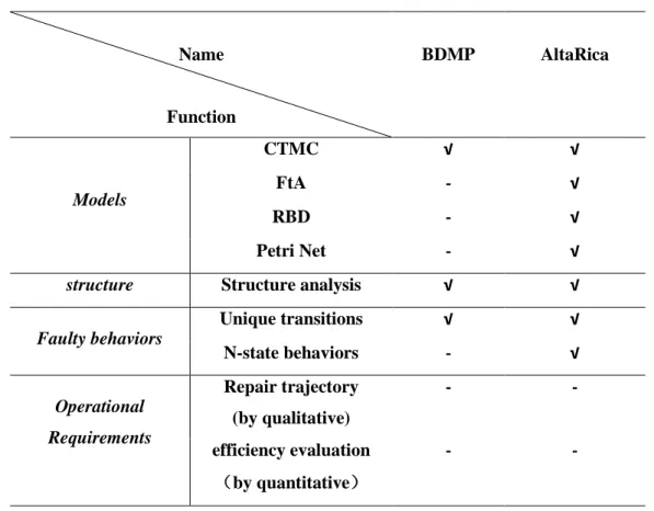
Table 1 Review of the model generation approaches ... 38

Table 2. Transition function of the composition result ... 48

Table 3. AP association function ... 50

Table 4. AP conjunction by the CTMC composition operation ... 51

Table 5. Management requirement satisfying transition function of SPA1 ... 62

Table 6. CCFT Validation of system sys1 ... 70

Table 7 CCFT Validation of system Sys2 ... 69

Table 8 Parameters of the components in power plant system ... 71

Table 9 CCFT Result ... 73

(15)

(16)

Research Motivation

Industrial systems are expected to fulfill their function while providing qualitative operation guarantees and reasonable confidence about their availability. They involve a large number of interacting components. Behaviors are by nature distributed, and the outputs of some components are fed into the inputs of the other components, according to a predefined structure. The structure of an industrial system covers two aspects. A functional aspect, where components interact in order to provide a global functionality, tackled by design engineers, whose concern is mainly providing the correct service in the expected time. Yet, the inherent complexity of these systems also comes from the number of constituting components and their individual reliability. Component failures may lead to unpredictable situations, synonym of malfunctioning or, for critical systems, to the serious hazard. Thus, a dysfunctional aspect concentrates a large part of the design efforts, and brings additional complexity to the system: additional components are supplied as backup and their operation needs accurate specification that is independent of the functional requirements of the global system. This design effort is compulsory in order to provide continuous operation guarantees and avoid the total breakdown. Moreover, the probability and impact of each failure, on the one hand, and of possible sequences of failures on the other hand, need to be accurately evaluated, so that appropriate maintenance actions can be scheduled. Hence, it appears to be interesting to associate operational requirements to conventional dependability requirements in order to assess typical service or recovery policies. This is the object of the operational dependability assessment.

Mathematical models have shown interesting features for analyzing failure mechanisms, and system dependability evaluation, which is the original intention of Model Based Safety Assessment, abbreviated MBSA[1, 2]. The word ‘safety’ in this context is a synonym to the dependability. In MBSA, the system is expressed by its faulty model. Based on this model, time-based indicators may be computed to assess the system’s operational dependability, such as the meantime to failure (MTTF), the meantime to repair (MTTR) and the mean time between failures (MTBF). Alternatively, availability, reliability and maintainability probabilities can also be computed.

Failures and repairs can be naturally sensed as events, occurring within a complex scenario. Hence, the discrete-event system modeling approach appears to be well suitable for expressing dysfunctional system models. Mature approaches rely on Stochastic Petri Nets[3] or Markov Processes[4], for indicators calculation, model checking or even simulation.

The BDMP (Boolean Logic Driven Markov Process) approach provides fault-tree based modeling in order to generate the underlying dysfunctional behaviors as a Markov process[5]. One of the BDMP’s

(17)

advantages is that it makes failure sequences explicit. For instance, the cold redundancy architectures are accurately modeled, because the redundant component failure may only occur after the failure of the primary component, and this is expressed by an appropriate failure sequence.

AltaRica[6] provides a powerful modeling solution under the form of guarded transition systems. AltaRica provides modeling flexibility through an opening towards other modeling languages, such as AADL, SysML and Event-B, for the purpose of enlarging the modeling domain and enhancing the safety assessment.

Beyond the approaches enumerated above, safety-critical systems need to be assessed according to four aspects: reliability, availability, maintainability and safety (RAMS)[1]. The reliability is the ability that a system continuously delivers its expected mission within a given time duration, without any failure occurrence. The availability is the ability that a system continuously delivers its expected mission within a given time duration, considering recoverable breakdowns. The maintainability denotes the ability that the system recovers from the totally broken down to be able to contribute to its attempted mission within a given time duration. The safety denotes the ability of the system to be harmless to human beings within a given time duration.

MBSA provides accurate reliability assessment work environment, provided that the underlying model complies with three requirements:

1. It is able to describe the whole dysfunctional behaviors. For a complex industrial system, involving several interacting components, each component should be modeled according to its dysfunctional behavior. The global behavior is obtained from the combination of local behaviors, according to a systematic structure which is designed for delivering the system service;

2. It is able to target specific configurations, and provide mechanisms to associate dysfunctional trajectories to these configurations, in order to compute dependability indicators. These configurations are usually modeled by states. For instance, a component model may feature several nominal operating states, such as idle, working, besides the breakdown state;

3. It is able to integrate additional requirements, such as qualitative or quantitative aspects. Qualitative requirements may be featured by precedence constraints or priorities. For example, in case several components are waiting for repair, the most important components should have the priority to be repaired first. Quantitative aspects are mostly related to costs of repair trajectories. Additional estimations of the resulting “health” of the repaired system may also be considered.

In order to guarantee the accuracy of the assessment, these aspects need to be expressed and handled formally. Yet, no research results exist up to now, offering dependability assessment features and handling in parallel the operational consideration of dependability. For example, the model generated from GRIF [7] or from AltaRica is short of an extension for these operational considerations.

(18)

In turn, BDMP is able to consider failure sequences starting with a trigger event, and also considers complex behaviors of the components (for example, success rate to turn on, and the behavior of ‘reconfiguration’), but does not provide the ability to integrate repair trajectory requirements.

This is why, the motivation of this research is to provide a unified approach for dependability assessment of structured systems taking into account trajectory requirements. Several formal modeling and transformation steps are advocated, handling successively the system’s structure and behavior.

The first step consists of a macroscopic assessment relying on the structure of the system at hand. The aim of this step is to identify how local component faults may impact on a possible global breakdown. Fault tree Analysis (FtA) is applied for the structural analysis and produces a failure statement for the global system, under the form of a logic expression. This expression illustrates the global breakdown configurations of the system at hand.

The failure of several certain components is necessary enough to cause the whole system broken down, which issues the minimal cut set. The combination of all the minimal cut sets constitutes the failure logic expression of this system.

The second step aims at relating exhaustively the global breakdown configurations to the component behaviors and local breakdowns which may collectively lead to a global breakdown. Each component behavior is modeled formally as a state based discrete event system. The global system behavior is obtained formally by combining the local behaviors of all components, by applying a state of the art composition operation. The global model obtained contains all the local component behaviors, and is able to exhibit any global breakdown configuration.

At this point, specific services such as repair requirements can be integrated. These are defined as behavioral models, possibly describing desired repair sequences or priorities, or other operational behaviors. The third step produces a global model which features these resulting behaviors in addition to the preceding one.

The fourth step aims at targeting global breakdown configurations in the behavioral model: the global breakdown statement is formally related to the system behavior, by an appropriate labeling procedure. The resulting labeled behavioral model features all the possible scenarios, containing local breakdowns and leading to a global breakdown.

Face to operational dependability, four objectives can be tackled:

1. Operational Reliability, by assuming no disturbance at the initial state and the accessibility to a total breakdown state, while including specific requirements for service or recovery;

2. Operational Maintainability, by considering that the system is initially totally broken down and the accessibility to a system healthily working state, including specific requirements for service or

(19)

recovery;

3. Operational Availability, by considering that the system is initially working, possibly experiencing failures and recoveries and including specific requirements for service or recovery;

4. Operational Safety, by providing a system design which implies no harmful situations for its human environment, while including specific requirements for service or recovery;

This work only focuses on Operational Reliability. Thus, each component can be reasonably assumed to “repairable”. Thus, breakdowns may be followed by repairs, with one exception for reliability: there is no possibility to recover from a total breakdown. In order to express this particularity, no repairs should be allowed in the global breakdown configurations. This requires an additional transformation of the labeled behavioral model, by making definitive all the global breakdown configurations.

The resulting system features event-triggered trajectories leading to a definitive global breakdown. These events are in general stochastically described by rates; hence a continuous-time Markov Chain is derived from the labeled behavioral model and offers the usual computations for reliability assessment.

Alternatively, beyond computing failure probabilities, it appears to be interesting to evaluate the effectiveness of the repair management policy. The framework presented in this work also proposes this feature, through quantitative cost simulation, relying on the event and/or global configuration costs.

In conclusion, this work provides a formal modeling framework, based on modular behavioral generation, able to assess the operational dependability of the system, by taking into account specific service or repair specifications and by evaluating their effectiveness. A quantitative analysis methodology is developed, for the calculation of the system capacity, taking into account the components failures.

(20)

Chapter 1 State of the art

This chapter contains two parts: First, the context of this research;

Second, the statement of the relative works.

(21)

1.1 Introduction

Industrial systems are expected to deliver a global service, and are designed from several interacting and possibly distributed components. The interactions between these components amount to either information, or material interdependencies. Each individual component is subject to failures and some components may be repaired. The impact of one component failure on the global service delivery may vary according to the interdependencies relative to this component. Thus, a component failure is not always a synonym of total breakdown with a definitive loss of the global service.

The guarantee of service continuity is generally critical in any industrial context. In order to provide such a guarantee, the failures of individual components and their possible impacts on the service delivery need to be assessed, and appropriate operations anticipated. Thus, the engineering of the global service needs to be completed by the modeling and evaluation of its reliability, availability and maintainability, issued from the knowledge provided by the failure assessment.

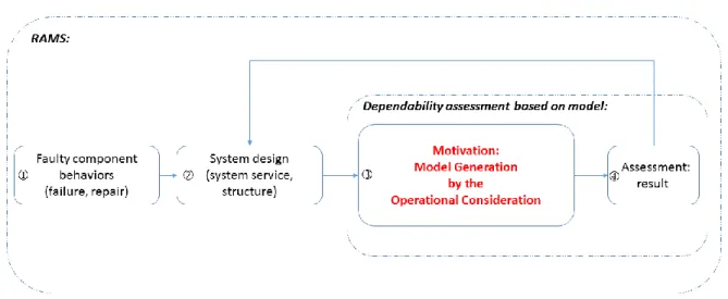
Figure 1 Dependable systems design flow

Figure 1 shows a usual system design flow encompassing both the functional and dysfunctional points of view [8, 9]. The accurate assessment of failure impacts requires several modeling stages:

1. the faulty component modeling step provides qualitative and quantitative knowledge about the faulty behaviors and their probability;

2. the system design step defines the structure and behavior of underlying components, as well as their interdependencies. The resulting system model may also highlight the behavioral impact of component failure on the global service expected;

3. the model-based dependability assessment step relies on both the system and component models. The assessment can be either qualitative or quantitative, and relies on dedicated formal tools for evaluating the overall continuity of the global service. This step provides both quantitative (mean time to failure or repair, failure probabilities, etc.) and qualitative results (corner-case failure scenarii

(23)

and their impact on the service expected).

In this chapter, Section 1.2 introduces the context of this research (  in the figure). Section 1.3 introduces the state of the art of this research motivation (  in the figure), in which the related theory extensions are studied and the typical model generation approaches are stated.

1.2 S

ystem Dependability

This section recalls the terms and concepts related to model based safety assessment. The Reliability, Availability and Maintainability (RAM) concepts, as well as their mathematical background (followed by the calculation method of time indicators) are presented in 1.2.1. The perimeter of the dependability notion used throughout this work is stated in 1.2.2.

1.2.1 Faulty component behaviors

In the context of possible fault occurrences, specific fault-related behaviors need to be considered. The Reliability is the ability of a system to continuously provide its expected service without breaking. The Availability denotes the system readiness for providing its expected service. The Maintainability denotes the ability of a system to be either maintained or repaired. Behind these intuitive and qualitative expressions, a mathematical framework exists providing their accurate definition and calculation. These are recalled in the sequel.

Assuming design and operational hypothesis, any system can be seen as one single component which can break and be repaired. Failures occur with an average rate denoted by ‘λ’, and repairs occur with an average rate denoted by ‘μ’. The system can be seen as featuring two states: a working state, denoted by S0, and the failed state, denoted by S1. Figure 2 represents the Continuous Time Markov Chain (CTMC) models of the three dependability notions stated above for the system at hand.

In a Reliability model, the system is assumed to be initially functional. The initial state is the working state S0. It may fail with a rate of ‘λ’, and follow the transition to the failed state S1. This model offers the basis for the calculation of Mean Time to Failure indicators.

In the Maintainability model, the system is assumed to be initially broken, hence the initial state is S1. The system can be repaired with an average rate of ‘μ’, returning to the working state S0. This model offers the basis for the calculation of Mean Time to Repair indicators.

In the Availability model, the system is assumed to be initially functional, and may fail and be repaired recurrently. Hence, the initial state is S0. Failures occur with a rate of ‘λ’. On a failure occurrence, the system model switches to state S1. Repairs occur with a rate of ‘μ’, and the system recovers its functional state S0. This model offers the basis for the calculation of Mean Time between

(24)

Failures indicators. Hence, these three models are representative for calculating the most conventional failure/repair mean time indicators[10-12].

Such representations focus essentially on the dysfunctional aspect of a system. Still, the model can represent both the system behavior in its extensive complexity, through various operating or idle states triggered by various nominal operation events, and its failure state, together with the specific failure/repair events. The initial state assumption defines the assessment framework: reliability, maintainability or availability. This is illustrated in Figure 2. Events {‘α’, ‘β’} related to a nominal behavior of the system coexist with the failure/repair events {‘ λ’,’ μ’}. States S0 and S1 model the idle and working system configurations, whereas state S2 models the breakdown.

Reliability, Maintainability and Availability can be assessed on these models by adequately setting the initial state: S0 for Reliability and Availability (Figures 2d and 2f), and S2 for Maintainability (Figure 2e).

Figure 2 RAM Markov chain model

1.2.2 System design: service and structure

The complexity management of an industrial system meant to provide service calls for advanced engineering skills and resources, at several levels:

1. system design: definition of the functional, logical and physical architecture through requirement analysis, functional analysis and decomposition, logical and physical component mapping; 2. system development: for each component, either design its behavior, or source it externally, verify

its correction, alone, and in progressive inclusion with the rest of the system;

3. system deployment: progressively set-up the system, according to a deployment plan, in consistent interaction with the ongoing activity[13];

(25)

These milestones appear to be sequential, but are strongly interdependent: the system operation calls for an acceptable and most of all qualified level of reliability, availability and maintainability (RAM). These aspects are orthogonal to the system service, they do not concern its nature but its continuity, which is why they may be easily overlooked.

A dysfunctional analysis phase [14, 15] can be lead in parallel with the system development phase, and often induces costly iterations in order to redesign components, due to the late identification of critical RAM aspects. The early integration and prediction of reliability, availability and maintainability features into the design flow [16, 17] is more recently advocated in order to consider dysfunctional aspects as soon as possible and hence, minimize the overhead of such redesign iterations.

Hence, a service provided by an industrial system universally relies on the interaction of services of its underlying components[18, 19]. These interactions materialize flows having the morphology of cascades, derivations, cycles, or a combination of these patterns. These patterns are identified as

structures, which can be either series, or parallel, or mixed. In a RAM analysis approach, a set of

interacting services must be mapped to such a structure. Most often, this preliminary step abstracts away the service nature and only focuses on the interdependence[20]. For instance, in a series structure, regardless of its nature, a global service requires that all local services be operating. In a parallel structure, the global service requires that at least one local service be operating. It is assumed, without loss of generality, that component failures are never simultaneous.

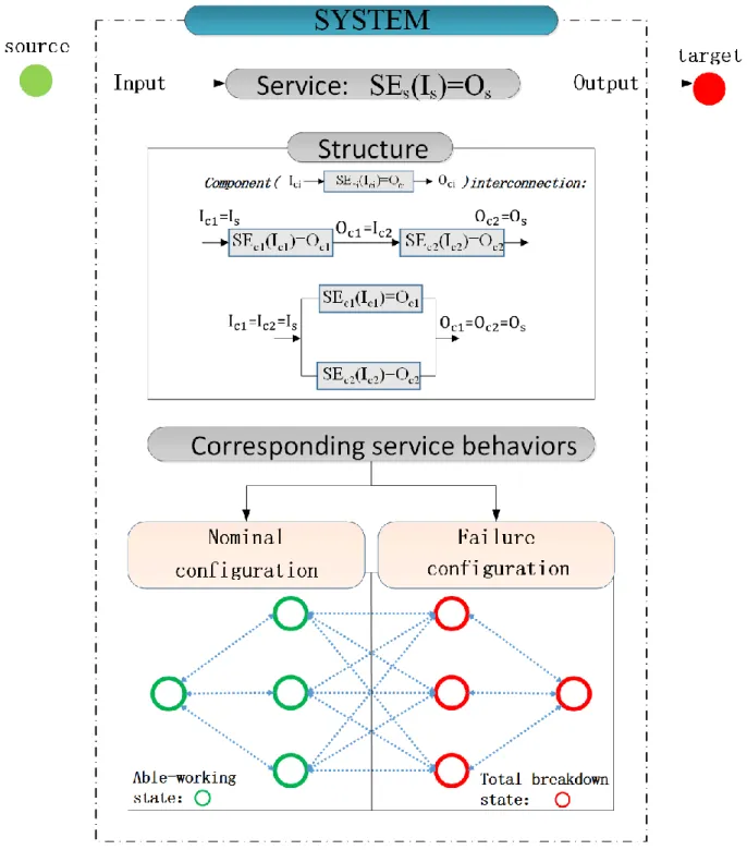
These aspects are summarized in Figure 3. Each system has a structure, materialized recursively by components and a specific interconnection. The specification of the interconnection between components is mandatory, as it determines qualitatively the RAM properties of the whole system. Hence, as shown in Figure 3, the system service amounts to processing an input flow, identified as the “source”, and produce an intended output, identified as the “target”. The source can consist of either physical materials, or primary resources, or machinery, or energy, or finance, etc. And the target should be an expected result, either material or immaterial.

Besides, the system structure also determines the dysfunctional behaviors that need to be anticipated. The global system behavioral model features a collection of configurations which are identifiable as able to work, or simply working configurations on one hand, and breakdown configurations, named total breakdown states, together with all the possible transitions between these configurations. It is interesting to notice that this model is exhaustive: it represents all the possible sequences compliant with its components’ behaviors. This makes it possible to reason about specific sequences expressing desired (realizable) behaviors, such as maintenance policies, prioritization, etc. Such requirements can be expressed by pruning inadequate sequences from system model, which is extremely error-prone. A separation between system and requirement specifications is of great interest.

(26)

Figure 3 system：structure and service

Hence, in order to perform a service, underlying components provide different services and form a structure which can be complex[21-23]. A component supposed to deliver its service, by transforming input Ici into output Oci is denoted as Ci. Its service function is 𝑆𝐸𝐶_𝑖:

SEci(Ici)=Oci,

The behavioral models highlighted in Figure 2 provide a high abstraction level, which makes them representative for virtually any service: states such as “working”, “idle” and “breakdown” can always

(27)

be identified both in a system or in its underlying components. Thus, a service SEci operates in its

“working” state of the underlying state-transition model of Ci. In this state, SECi is nominally provided.

A system S is constructed by interconnecting its underlying services. For a system S providing a service SEs relying on components {𝐶₁, 𝐶₂, … , 𝐶_𝑁 }, this is achieved by adequately mapping service

outputs Ocj of component 𝐶𝑗 to the corresponding input Ici of component 𝐶𝑖 according to the desired

interconnection.

Probing the availability of a system at a given moment is not always obvious. Yet, it is assumed in this document that when a system is broken down, it ceases to deliver its service. Its output is undefined, denoted ⊥. Hence, all components are considered fail-silent. Thus, a service produces an expected output, if it is operational, and ⊥ if it is broken down:

𝑆𝐸𝐶𝑖(𝐼𝐶𝐼) = {

𝑂𝐶𝑖 𝑖𝑓 𝐶𝑖 𝑖𝑠 𝑜𝑝𝑒𝑟𝑎𝑡𝑖𝑜𝑛𝑎𝑙 ⊥ 𝑖𝑓 𝐶𝑖 𝑖𝑠 𝑏𝑟𝑜𝑘𝑒𝑛 𝑑𝑜𝑤𝑛

In the sequel, for consistency reasons, the following conditions should be assumed:

1. For any component 𝐶, 𝑆𝐸𝐶(⊥) = ⊥

2. For any component 𝐶, if 𝐶 is broken down, then 𝑆𝐸𝐶(𝐼𝐶) = ⊥. The reciprocal is not true: the output

of a component can be undefined because of a component breakdown in its transitive fan-in. 3. For a collection of k flows 𝐹 = {𝑂1, 𝑂2, … , 𝑂𝑘} it is useful to denote that:

𝐹 = ⊥ 𝑖𝑓𝑓 ∀𝑖 = 1 … 𝑘: 𝑂𝑖 = ⊥

Based on the two basic system structures, series and parallel, various complex structures can be built, yielding either well-known architectures, such as the cold-redundancy structure, the warm redundancy structure, the vote structure, the mixed structure, or more typical structures.

Thanks to the system representation as a structure of components, the global RAM features can be formalized and assessed in terms of the RAM of its components.

Hence, the notion of total breakdown can be defined in terms of local components’ breakdowns and the system structure. The same holds for the system reliability, availability, and maintainability, which can be assessed globally, based on its structure and the behavioral model of each component.

The following paragraphs recall several conventional system structures [10, 24-27].

A. The series structure

This structure features a system 𝑆 made of a set of 𝑁 components 𝐶1, 𝐶2, … , 𝐶𝑁 , fed by the

source flow according to the following interconnection:

(28)

 ∀ 𝑖 ∈ 2 … 𝑛 ∶ 𝐼𝑖= 𝑂1−1;

 𝑡𝑎𝑟𝑔𝑒𝑡 = 𝑂_𝑁 .

Figure 4 series structure system. The system’ service results from the cooperating service of all components, where not a single component may fail.

Figure 4 series structure system

The output of 𝑆 is either the output of 𝐶𝑁 or ⊥. For the series structure, we have

𝑆𝐸𝑆≠⊥ 𝑖𝑓𝑓 ⋀ 𝑆𝐸𝐶𝑖

𝑁

𝑖=1

≠ ⊥

The service of S cannot be provided if at least one of the local components is not able to contribute its own service.

B. The parallel structure

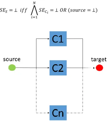
To enhance the availability of the system’s service or to enhance its production, several similar components are distributed to work side by side sharing the same input and producing the same output. On the view of the dependability, this designing method empowers the system by the ability of fault tolerant.

This structure features a system 𝑆 made of a set of 𝑁 components 𝐶1, 𝐶2, … , 𝐶𝑁 , fed by the

source flow according to the following interconnection:

 ∀𝑖 = 1 … 𝑁 ∶ 𝐼𝑖= 𝑠𝑜𝑢𝑟𝑐𝑒;

 ∀ 𝑖 ∈ 1 … 𝑛 ∶ 𝑂_𝑖= 𝑆𝐸( 𝐼1);

 𝑡𝑎𝑟𝑔𝑒𝑡 ∈ 2₁{𝑂1,𝑂2,…𝑂𝑁}_.

Figure 5 illustrates the service of this system. To realize its service, its structure is constructed by n components denoted by C1, C2 …Cn. These components share the same input and this input is also the system input (marked by the ‘source’ in the figure): and they contribute to the same output (marked by the ‘target’ in the figure) as to be the output of the system [21-23]

The components working in the parallel structure system, often provide the same service, treating the same input and producing the same or similar outputs. However, the capacity of the components’

(29)

service may differ (shared load). So, the parallel structure can be considered as a redundancy-based design, where the components may have different service capacities. If some components fail, the system partially loses its capacity, but is still able to deliver its service function. Thus, in case that at least one of these components is able to work, the whole system is able to provide its function. In case that all the components lose their functions, this system is totally broken down.

Thus, for the parallel structure, it can be stated that:

𝑆𝐸𝑆= ⊥ 𝑖𝑓𝑓 ⋀ 𝑆𝐸𝐶_𝑖 𝑁

𝑖=1

= ⊥ 𝑂𝑅 (𝑠𝑜𝑢𝑟𝑐𝑒 = ⊥)

Figure 5 Parallel structure system

The service of this system cannot be provided if its input is undefined or if all of its components are unable to provide their service, because they are broken down.

Based on the equation above, the more components collaborating in the parallel structure system, the stronger ability to deliver the global service is. According to this, one method to enhance the system reliability is to set a redundant component (to build a parallel structure), assisting the major working components[28], which will be further introduced in the following parts.

(30)

C. The cold-redundancy structure

Figure 6 Cold redundancy structure

The structures recalled above can be combined and adapted, in order to obtain additional, possibly enhanced reliability features. Thus, in order to guarantee the availability of the system’s service and empower its the fault tolerance, besides a main operating component there is an equivalent reserve component, ready for operation, and which can be triggered in case the main component breaks down. Figure 6 illustrates this structure. It is generally assumed that the switch is fault-free. Yet, the non-commuting probability is not zero, related to a possible lack of switching command. The services of 𝐶1 and 𝐶2 are considered equivalent. They share the same input and contribute to the same output.

Component 𝐶1 is the main component: Is=Ic1 and Os=Oc1. If 𝐶₁breaks down, component 𝐶₂ is switched

on and starts to work instead of 𝐶1 : Is=Ic2 and Os=Oc2. This structure and use is known as cold

redundancy. The service provided 𝑆𝐸𝑆 is expressed in the same way as for the parallel structure.

D. The warm redundancy structure

Figure 7 Warm redundancy structure

Simarly but not the same with the parallel structure, a redundancy structure always features an accompanying component working beside with a main component, and these two components have the same service function with the same input and output. However, the production capacity of the accompanying component is often weaker than the main working component. With respect to the parallel structure, the warm redundancy structure is rather operational: enhance the service availability till the main component is repaired or replaced.

Figure 7 illustrates a warm redundancy structure featuring a main component 𝐶1 and a redundancy

(31)

and they produce the same output (for the target). The service provided 𝑆𝐸𝑆 is expressed in the same

way as for the parallel structure.

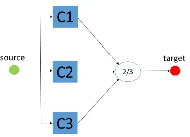
E. The voting structure

Figure 8 Vote structure system

The voting structure system is made of three or more components which are expected to provide identical service but which can differ in terms of either design, manufacturing, or sourcing. With the assumption that the voting engine is considered to be always perfect, the output of this system amounts to a decision made by voting engine: each component asserts its own output; the output asserted and shared majority between the components shall be the output of the system. In practice, voting structures contain three decision making components, as shown in Figure 8, which is the minimum in order to guarantee the majority.

Thus, components C1, C2 and C3 receive the same input. Their output is a decision and is submitted to voter which achieves the actual voting. If at least two components are healthily working, the system is able to deliver its service. It is important to note that in a voting architecture, components 𝐶1, 𝐶2, 𝐶3

are not supposed to be fault-silent. A fault is rather synonym of a “wrong” decision, rather than an undefined output. The structure is fault tolerant, as long as the three components produce outputs. Hence, the service breakdown of this system is defined as:

𝑆𝐸𝑆= ⊥ 𝑖𝑓𝑓 ⋁ 𝑆𝐸𝐶𝑖

𝑁

𝑖=1

= ⊥ 𝑂𝑅 (𝑠𝑜𝑢𝑟𝑐𝑒 = ⊥)

(32)

F. The series-parallel structure

Figure 9 Series-Parallel Structure

The basic and regular structures recalled above can be combined in order to achieve more complex architectures, as shown in Figure 9. Such structures can use single components, such as 𝐶1,

which is used alone because it is considered very reliable, or simply very expensive, and also other components operating in redundancy, in order to provide higher performance, or reliability, or both. These structures are recursively analyzed, by identifying their subcomponents with simple structures (series, parallel, …).

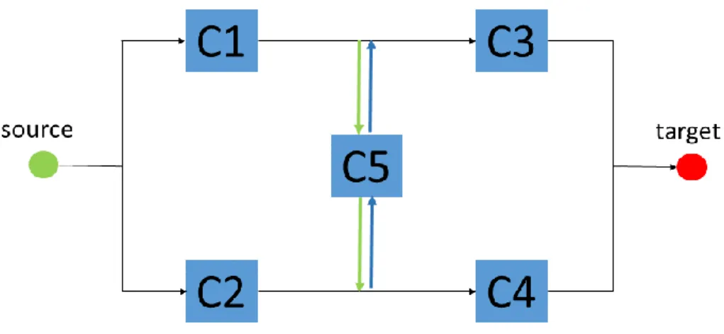
G. Mixed Structure

Figure 10 Mixed Structure

More complex flows can be defined and compose a mixed structure. The ‘mixed’ feature emphasizes that there may exist different interactions among the components and that these interactions amount to various superposed structures.

The example shown in Figure 10 features components C1 and C2 which share the input (source in the figure) of the system : Is=IC1, Is=IC2; components C3 and C4 both contribute to the output of the

system(target in the figure) : Os=OC3, Os=OC4; component C3 treats the output of C1 : OC1=IC3;

component C4 treats the output of C2 : OC2=IC4. However, component features a cyclic dependency: it

(33)

processes the output of C2 and outputs its result to C3: IC5=OC2, OC5=IC3. Again, these dependencies

have a decisive impact on the dysfunctional behavior of this structure.

1.3 Model based dependability assessment: state of the art

Discrete Event Systems (DES) offer a helpful abstraction level for modeling and assessing system dependability. They feature transitions which can be driven by either probabilities, rates or events, are which can be used to model failure behaviors. Discrete states are used to represent the possible configurations of the system. Failure scenarii are represented by sequences of transitions between identified initial state and a pre-designed failure configuration. They provide qualitative information about failure occurrences. If quantitative figures are available, modeling consistently event-related probabilities or rates, quantitative dependability indicators can be further calculated. The discrete event system modeling approaches, such as Stochastic Petri nets and Markov chains are well suitable for this modeling. DES models are usually modeled by hand. Yet, in order to encompass the potential complexity due to the growing size of a system, the ability of systematic generation of global, complex reliability models from basic ones appears to be vital.

In order to discuss the Discrete Event System model generation approaches, the ordinary dependability assessment methodologies are briefly recalled in the following. Hence, it is worth being recalled that DES models provide a behavioral point of view of the system at hand, which help in both identifying breakdown states and numerically assessing the reliability. These are possibly used in synergy with models and methods representing structure and hierarchy such as the Fault tree Analysis (FtA) and Reliability Block Diagram (RBD) analysis. FtA is a top-down tree logic modeling method. The leaves which stand for the failure of the components are connected by the logic gates (‘and’ gate for parallel structure, ‘or’ gate for series structure, etc), and the result is evaluated on the top of the fault tree [29]. In RBD, blocks are used to present the components, and the blocks are connected with the series network and parallel network. The detailed methodology of FtA and RBD is studied in a subsequent section dedicated to GRIF.

In the sequel, contributions of the Discrete Event Systems domain to the Model Based Safety Assessment are stated, in section 1.3.1, and focused on MBSA generation approaches, in section 1.3.2.

1.3.1 Discrete Event System Theory Contribution to MBSA

Two main modeling approaches are recalled: modeling token flows using Stochastic Petri Nets (SPN) and modeling sequences using Continuous Time Markov Chain (CTMC). In order to compute the ordinary time indicators, four subsequent operations need to be recalled:

(34)

- structural analysis, in order to determine the failure logic;

- state combination, in order to reduce the model size by regrouping states according to a quantitative rate equivalence notion;

- CTMC to stochastic Petri net transformation. Stochastic Petri nets own the advantage of modeling traceability.

The objective for inserting the DES theory into MBSA are based on its main abilities for both model generation and proof. Generation amounts to automatically delivering of a model thanks to composition. This ability is intensively used when handling complexity. The proof amounts to validating sequence and structure through properties statements such as observability and accessibility to specific states such as TBS's.These elements are recalled in the next two sections.

A. Continuous Time Markov Chains for system assessment

This part recalls the reliability Markov chain modeling methodology. An example is used to explain how to calculate the time indicator MTTF (Mean time to Failure). Behavioral and structural modeling are illustrated, together with the behavioral model composition.

CTMC modeling principle based on the system structure

Named after the Russian mathematician Andrey Markov (1856-1922), Markov chains model stochastic processes by expressing quantitatively transition relations between the states of the system. The Markov stochastic processes are memoryless: the next state only depends on the current state regardless of any past evolution [30, 31]. The Continuous Time Markov Chains (CTMC) express state transitions by relying on event occurrence rates [32, 33]. For instance, the failure rate represents the average number of failure occurrences by time unit.

For a given system satisfying the Markov memoryless property, a CTMC model is achievable and thus, an equivalent transition matrix can be derived, which allow the calculation of time indicators [10, 34-37].

As depicted in section 1.2.2, beyond the individual RAM indicators of each component, the system structure also has an impact on the global MBSA results. The expected results for MBSA would be the possibility to discuss on a better construction of service and/or better specification for the failed system face to the repair management.

Behind each system structure there is a static and a dynamic perception. The structure in itself is a static statement, unable to express the possible scenarii leading to partial and/or total breakdowns. Such scenarii are expected to express the actual run of a sequence of configurations, leading to a particular situation, such as a breakdown. This is a modeling gap which is conveniently filled by the CTMC modeling, in order to express the global dysfunctional behavior from individual ones. The behavioral model abstracts away most functional states and focuses on the dysfunctional aspects: component models usually feature two, maybe three kinds of states expressing inactivity, working and breakdown.

(35)

Inactivity and working states are sometimes grouped into a single state expressing the absence of breakdown.

Example

Figure represents two possible structures achievable from two individual components, C1 and C2, modeled by subfigures 12(a) and 12(b). Each component presents two states: a working state, denoted respectively by W1 and W2, and a brokendown state denoted respectively by B1 and B2. For i=1..2, component Ci can break down with a failure rate λi. Each component can be repaired by a service engineer, and the repair average rates are denoted μi.

Figure 11 Basic reliability CTMC models from structure definitions

Thus the system features globally four possible states: ‘W1.W2’ meaning C1 and C2 and both working; ‘W1.B2’ meaning C1 is working but C2 is broken down; ‘B1.W2’meaning C1 is broken down

(36)

however C2 is working; ‘B1.B2’meaning both C1 and C2 are broken down. And, the evolution of the system states are driven by the failure rates and the repair rates of the components (λi and μi).

A series structure can be built by connecting the output of C1 with the input of C2, as shown in Figure 11.c. This interconnection requires that both components are operational: if either component breaks down, the global system service cannot be achieved anymore. Similarly, if C1 and C2 could share the same inputs and feed the same output, a parallel structure can be built, as shown in Figure 11.e.

The reliability CTMC model of the series structure is represented in Figure 11.d. This model represents the possible scenarii leading to the global, total breakdown, as defined in section 1.2.2.

It can be observed that only when these two components are operational, i.e in their working state Wi, the system is globally operational. If one component breaks down, the whole system is broken down. So, the system states associations ‘W1.B2’, ‘B1.W2’ and ‘B1.B2’ are the system’s Total Breakdown States (abbreviated TBS in the figure).

The reliability CTMC model of the parallel structure is presented in Figure 11.f. This model represents the possible scenario leading to the global, total breakdown.

It can be observed that only when components C1 and C2 are both broken down, the system is totally broken down. So, the system state association B1.B2 represents the TBS.

Notice that the behavioral models obtained here are meant to assess reliability. Hence, they do not entirely feature all the possible behaviors. In theory, it should be possible to leave the TBS by repairing either one or both components, according to their local configuration. Still, in order to assess reliability, the global model should exclusively feature the scenarii leading to the total breakdown. As shown in Figure .c, for the parallel structure, repair actions can occur arbitrarily often, but only as long as the system is globally available.

Hence, reliability CTMC models are usually manually established from the system structure and from the knowledge about the individual component dysfunctional behaviors. This process requires a high level of expertise, as it is done manually, as advocated by[7, 38]. It can be apprehended for medium sized systems, but becomes error-prone as soon as the structure gets complex. The ability of systematically compose CTMC models appears to be fundamental in order to handle this complexity.

CTMC composition

This operation builds a global behavioral system model out its components. It is based on the theory of interactive Markov chain[39]. Ordinary CTMC models express event occurrences quantitatively, as rates. The notion of interactivity goes back up to events, and the possibility that the same event can impact the dynamics of more than one model. Besides that, component states are regrouped into global states

(37)

according to a Cartesian product approach. The transitions of the global model reflect all transitions of the underlying components. They reflect two kind of situations:

- asynchronous evolution, if a transition only occurs locally in a component CTMC model;

- synchronized evolution, if the transition is shared between two or mode component CTMC models, through the same event [39-41].

Figure 12 composition operation of interactive Markov chain

Example

Figure 12 shows a system built from two components 𝐶1 and 𝐶2. States W1 and W2 model

working configurations, B1and B2 model broken down configurations. It is assumed that failure and breakdown events cannot be simultaneous. The model expresses the fact that components 𝐶1 and 𝐶2 are

somehow interdependent, and that the same fault causes their common breakdown. This is denoted by label ‘commonbreak’ in the model. But each component can be repaired independently. The equivalent behavioral model is shown in Figure 2, denoted C1//C2. This model represents the whole system behaviors. The transition “repair1” and “repair2” are asynchronous. The transition “commonbreak” is taken synchronously by the two components.

(38)

State combination in CTMCs

Figure 13 State combination

As CTMCs are quantitative models, it is sometimes possible to regroup states. For a system composed of two failure/repairable components, 𝐶1 and 𝐶2, having both a failure rate of “λ” and a repair

rate of “μ”. In order to deliver the service of the system, these two components are working independently, which means they do not influence each other. According to Figure 13 c, states B1W2 and W1B2 express respectively the fact that 𝐶1 or 𝐶2is broken down. This situation can be simplified,

by expressing the fact that either 𝐶1 or 𝐶2 are faulty, using an equivalent state W1.B2-B1.W2 in Figure

13.d.

According to[42-44], transitions from state x to state y are fired with a probability Px,y. Let A

and d be CTMC states, and 𝑑1, 𝑑2, … 𝑑𝑛 be states to be combined into d. In the resulting state-combined

CTMC’ the transition probabilities are calculated as follows:

𝑃𝐴,𝑑 = 𝑃𝐴,𝑑1+ 𝑃𝐴,𝑑2+ ⋯ + 𝑃𝐴,𝑑𝑛

(39)

Thus, the transition rate from W1.W2 to W1.B2-B1.W2 is:

𝑃𝑊1𝑊2,𝑊1𝐵2−𝐵1𝑊2= 𝑃𝑊1𝑊2,𝑊1𝐵2+ 𝑃𝑊1𝑊2,𝐵1𝑊2= λ. 𝑑𝑡 + λ. 𝑑𝑡 = 2λ. dt

The transition from W1.B2-B1.W2 to W1.W2 is:

𝑃𝑊1𝐵2−𝐵1𝑊2,𝑊1𝑊2= (𝑃𝐵1𝑊2,𝑊1𝑊2𝑃𝑊1𝑊2,𝐵1𝑊2+ 𝑃𝑊1𝐵2,𝑊1𝑊2𝑃𝑊1𝑊2,𝑊1𝐵2)/

𝑃𝑊1𝑊2,𝑊1𝐵2−𝐵1𝑊2=(λ. 𝑑𝑡.μ.dt+λ. 𝑑𝑡.μ.dt)/2λ. dt = μ. 𝑑𝑡

And the other transition rates respect the same principle [44-46].

Discussion

In conclusion, Continuous time Markov chain models offer attractive abilities for quantitative and qualitative modeling of component and system behavior. They are able to model sequences, and offer accurate mechanisms for identifying critical components within a given structure. They are useful but not entirely appropriate in order to handle operational dependability into MBSA. The shortcoming mainly comes from three points:

- they do not offer a unique modeling framework to natively model structure, component and system behavior;

- they are not systematically able to specify MBSA-related behavioral requirements. For instance, a repair sequence between two or more components can be preferred. Its expression within the system CTMC model is tedious and error-prone. Still, this is a fundamental requirement for operational dependability;

- the state combination and simplification may lead to losing necessary behavioral information and decrease the level of accuracy for the dependability assessment. Indeed, states are necessary for modeling the various system configurations, such as idle, working or failure. Unless components feature identical dysfunctional behaviors, these could by lost through state combination, and reasoning about them would not be possible anymore. Similarly, transitions should not be regrouped, so that it remains possible to distinguish different transition rates in a system or even event sequences. This is why this work advocates not to use this particular simplification step, and in the sequel states shall not be combined. The loss of insight is compensated by the modular modeling methodology, which is able to reduce the modeling workload. The same modular approach is able to naturally integrate operational requirements inside the system model.

The following section recalls the usage of Petri Nets in the MBSA domain.

B. Petri nets for system assessment

Petri net models are equally helpful in dependability assessment[47, 48]. Together with Reliability Block Diagrams, Fault Tree Analysis and Markov chains, stochastic Petri nets (by the creation of

(40)

stochastic activity networks) and Timed Petri nets (by real-time faulty systems describing) were applied to dysfunctional system modeling[49, 50]. This approach is further improved by system failure sequence analysis[51] by graphical description [52] by the association of minimal cut sets in the system failure logic expression[53] and by aging tokens creation[54].

This section recalls the dependability assessment solutions using Stochastic Petri nets. The Petri net interconnection operation is recalled first, which can generate the system model based on the component behaviors. The Petri net modeling principle is subsequently recalled. Then, the transformation principles between CTMC and Petri nets are recalled. A discussion concerning Petri Net MBSA is presented at the end of this section.

Interconnection of Stochastic Petri net models

According to the research motivation presented above, the global system behavior needs to be built out of its individual components. Thus, the composition of the individual models in order to generate the system model is a required step. Moreover, additional behavioral specifications need to be modeled and composed into the global result. Petri nets can be composed by using the interconnection operation[55]. As illustrated in Figure left side, a connecting arc is used to link from one place in LPN (Local Petri Net) A to one transition in LPN B. By this method, these two local models are connected to form a global model. Another illustration is shown in Figure right side, an Interaction Petri Net (IPN) is used to connect from one transition in LPN A to two transitions in LPN B. Similarly, Local Generalised Stochastic Petri Nets are composed by modules with interconnection[56]. Subnets of Coloured Petri nets are also able to be composed according to their hierarchy [57]. The Petri nets components composition semantics are created in [58]. In the aboves solutions, tokens are exchanged in order to achieve the composition. Differently, in [55, 56] the composition operation is not impacted by the component tokens.

Figure 14 Interaction of Petri Net

Petri net modeling from the system structure

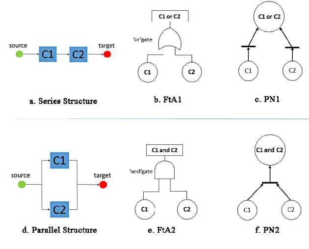
In order to to express the causality induced by the system structure, previous research works have focused on the dependability assessment using Petri nets[59-65]. The structural modeling principle of Petri Net is recalled in this part.

(41)

Figure 15 Petri Net model generation based on structure and FtA

Fault tree Analysis (FtA) and Petri nets can be combined in order to generate the system behavioral model. For example, the work of [60, 64, 65] uses Fault tree Analysis transformed into Petri nets and calculate the system indicators by the application of fuzzy Lambda-Tau methodology.

In Figure 15, the upper side presents the Petri net dysfunctional model corresponding to a series structure; the lower side presents the Petri net generation based on parallel structure system. There are two components A and B in the system, and the names ‘C1’ and ‘C2’ in the FtA are used to denote the failure state of the components. For the series structure, the ‘or’ gate FtA is established. And the ‘or’ gate of the FtA can be transformed into an ‘or’ Petri net structure (on the right side), expressing the fact that the failure of ‘C1’ or the failure of ‘C2’ is able to cause a total breakdown. For the parallel structure, the ‘and’ gate of the FtA can be transformed into an ‘and’ transition of Petri net, expressing the fact that the failure of ‘C1’ and the failure of ‘C2’ occurring both are able to cause a total breakdown.

Generalized Stochastic Petri nets

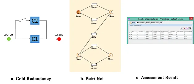
Generalized Stochastic Petri nets can be translated into Markov chains, which has the potential application for generating dependability models. A cold-redundancy model is used to illustrate this generation approach.

(42)

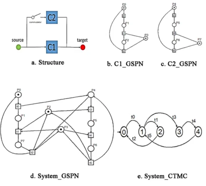
Example

Figure 16.a represents two components and one repairer. The repairer is only able to repair one component at a time. In case the component C1 is broken down, C2 starts to work instead. It is assumed that component C2 has the priority to be repaired over C1. After all these two components are successfully repaired, the repairer becomes idle.

The Generalized Stochastic Petri nets of components C1 and C2 are shown in Figure <C1_PN> and <C2_PN>. The edges and places are explained as following:

P0: C1 is operating; P4: C2 is operating;

P1: C1 is waiting for being repaired; P5: C2 is waiting for being repaired; P2: C1 is being repaired; P6: C2 is being repaired;

P3: repairer is available for C1; P7: repairer is available for C2; t0: C1 is broken down; t3: C2 is broken down; t1: repairer begins to repair C1; t4: repairer begins to repair C2; t2: C1 is successfully repaired; t5: C2 is successfully repaired;

Based on the component’ models, according to the repair principle of the system (C2 has the priority to be first repaired, if these two components are both breakdown), the global model is able to be generated by the model-interconnection. The Generalized Stochastic Petri Net of this system is represented in figure. d System_GSPN.

An example of the global expected behavior shows for instance that in place P2 if the two components break down, C2 has the priority to be repaired.

The Generalized Stochastic Petri can be translated into a Reachability Graph, according to [66-68]. In this example, the approach proposed by [69, 70] is used. The Petri Net Analysis tool ‘Tina’ performs the reachability analysis.

The generated CTMC is shown in the <System_CTMC> subfigure. The transition labels conserve the same meaning as in <System_GSPN>. The CTMC obtained reflects the initial system’ dysfunctional behavior: cold redundancy with two components, one repairer, C2 has the priority to be repaired.

(43)

Figure 16 transformation between Stochastic Petri Net and CTMC

Petri nets offer a complete modeling framework encompassing dysfunctional aspects and, able to generate equivalent CTMC models ready to be exploited by MBSA. Yet, according to the research motivation stated in this document Petri nets conserve some drawbacks that are discussed below.

Discussion

The main advantage of Petri nets comes from their compositional ability for generating the system model, as well as their natural ability to integrate the system structure in the behavioral model. Yet the following points remain to be investigated:

- though Petri net are able to consider the modeling of failure sequences, the manual expression of the global interleaving is difficult and error-prone. The integration of specifications for desired repair sequences is an additional difficulty;