Shape reconstruction of deposits inside a steam generator using eddy current measurements

HAL Id: tel-03144631

https://tel.archives-ouvertes.fr/tel-03144631

Submitted on 17 Feb 2021

HAL is a multi-disciplinary open access

archive for the deposit and dissemination of

sci-entific research documents, whether they are

pub-lished or not. The documents may come from

teaching and research institutions in France or

abroad, or from public or private research centers.

L’archive ouverte pluridisciplinaire HAL, est

destinée au dépôt et à la diffusion de documents

scientifiques de niveau recherche, publiés ou non,

émanant des établissements d’enseignement et de

recherche français ou étrangers, des laboratoires

publics ou privés.

Shape reconstruction of deposits inside a steam

generator using eddy current measurements

Hugo Girardon

To cite this version:

Hugo Girardon. Shape reconstruction of deposits inside a steam generator using eddy current

mea-surements. Modeling and Simulation. Institut Polytechnique de Paris, 2020. English. �NNT :

2020IP-PAX086�. �tel-03144631�

574

NNT

:

2020IPP

AX086

_{a steam generator using eddy current}

measurements

Th `ese de doctorat de l’Institut Polytechnique de Paris pr ´epar ´ee `a Ecole Polytechnique ´

Ecole doctorale n◦_{574 Ecole Doctorale de Math ´ematiques Hadamard (EDMH)}

Sp ´ecialit ´e de doctorat : Math ´ematiques appliqu ´ees Th `ese pr ´esent ´ee et soutenue `a Palaiseau, le 18/12/2020, par

H

UGO

G

IRARDON

Composition du Jury :

Fr ´ed ´eric Nataf

Directeur de recherche, Universit ´e Pierre et Marie Curie (LJLL) Pr ´esident

Nuutti Hyv ¨onen

Professeur, Aalto University (Department of Mathematics and

Systems Analysis) Rapporteur

S ´ebastien Pernet

Maˆıtre de recherche, ONERA (DTIM) Rapporteur

Sonia Fliss

Maˆıtre de conf ´erences, ENSTA ParisTech (UMA) Examinateur

Pierre Jolivet

Charg ´e de recherche CNRS, ENSEEIHT (IRIT) Examinateur

St ´ephanie Lohrengel

Maˆıtre de conf ´erences, Universit ´e de Reims Champagne-Ardenne

(Laboratoire de Math ´ematiques) Examinateur

Houssem Haddar

Directeur de recherche, INRIA Saclay (D ´eFI) Directeur de th `ese

Lorenzo Audibert

Remerciements

Apr`es avoir souffert pour produire ce splendide manuscrit de th`ese, me voici arriv´e `a la derni`ere

rubrique, qui paradoxalement se trouve plac´ee au d´ebut, les remerciements. Une vaste affaire que

de remercier toutes les personnes que j’ai pu croiser au gr´e de cette grande aventure qu’aura ´et´e ma

th`ese, tant elles sont nombreuses.

Mes plus grands remerciements vont bien entendu `a mon directeur de th`ese, Houssem Haddar et

mon tuteur `a EDF, Lorenzo Audibert. Bien souvent il m’a ´et´e conseill´e de bien faire attention au

choix des directeurs et co-encadrants pour sa th`ese, parfois mˆeme plus que le sujet lui-mˆeme, et je

dois avouer que j’ai eu beaucoup de chance de vous avoir pour encadrants. C’est grˆace `a vous que j’ai

pu arriver o`u j’en suis aujourd’hui et je vous en suis redevable. Mais au-del`a de l’important apport

scientifique que vous avez pu me donner pour progresser dans ma th`ese, votre bonne humeur, vos

taquineries ont cr´e´e `a mes yeux une bonne ambiance et bonne entente qui m’aura stimul´e pendant

ces trois ann´ees. Je tiens `a remercier ´egalement Lorenzo pour sa disponibilit´e `a toute ´epreuve, que

ce soit pour aller regarder avec moi le code pour y trouver un bug (ce qui me rappelle que je te dois

beaucoup de pains au chocolat), pour discuter de nouvelles id´ees `a apporter `a la th`ese ou d’EDF en

g´en´eral. Tu auras rempli ton rˆole de co-encadrant `a la perfection, voire mˆeme plus en m’aidant pour

la pr´eparation de mon avenir post-th`ese, ou bien mˆeme par de petites attentions qui m’ont beaucoup

touch´e.

Je tiens ´egalement `a remercier Pierre Jolivet, le r´ef´erent calcul haute performance devant l’´eternel

pour son int´erˆet sans faille depuis notre premier contact aux FreeFEM Days. Tu m’as apport´e une

aide tr`es pr´ecieuse pour la deuxi`eme partie de ma th`ese, pour la parall´elisation du code. Peu importe

l’heure, peu importe le jour, tu ´etais toujours prˆet `a r´epondre `a mes questions, parfois basiques, parfois

plus complexes. Grˆace `a toi j’ai acquis beaucoup de connaissances dans le domaine de l’informatique

en g´en´eral, et du calcul scientifique haute performance plus pr´ecis´ement. Cela aura ´et´e un plaisir

d’avoir fait ta connaissance et d’avoir ´ecrit un article avec toi. Je suis heureux que tu aies accept´e

d’ˆetre jury `a ma soutenance de th`ese. Un grand merci `a S´ebastien Pernet et Nuutti Hyv¨onen d’avoir

accept´e d’ˆetre les rapporteurs pour mon manuscrit, et `a Fr´ed´eric Nataf, Sonia Fliss et St´ephanie

Lohrengel de faire partie du jury.

Je voudrais par ailleurs adresser un grand merci `a Charles Dapogny pour son apport sur les

m´ethodes `a base de Level-Set, ainsi que Florian Feppon pour ses conseils avis´es sur la mˆeme th´ematique.

Les discussions que j’ai pu avoir avec vous deux m’auront sans aucun doute aid´e dans mes travaux

de th`ese.

Ayant fait une th`ese CIFRE `a EDF R&D et l’Ecole Polytechnique, je me dois de remercier les

diff´erentes entit´es qui m’auront accueilli pendant ces trois ans. A l’Ecole Polytechnique, je tiens

d’abord `a saluer mes co-bureaux, Marin Boyet, Florian Bourgey, Mehdi Talbi, Omar Saadi, Jaouad

Mourtada, Tristan Roget et plus particuli`erement Mathilde Boissier qui travaillait ´egalement sur des

probl´ematiques d’optimisation de forme et qui a apport´e sa contribution d’une certaine mani`ere `a ma

th`ese. Merci ´egalement `a l’´equipe INIRA D´eFI qui h´ebergeait ma th`ese, notamment Lucas Chesnel

pour sa bonne humeur et son sourire et Marcella Bonazzoli pour sa gentillesse et ses connaissances

en calcul hautes performances. Dans l’´equipe administrative, je tenais `a remercier Nass´era Naar,

Alexandra Noiret pour l’Ecole Polytechnique et Marie En´ee pour INRIA Saclay, pour votre efficacit´e

et l’aide que vous m’avez apport´ee pour les diff´erentes r´e-inscriptions en th`ese.

Du cˆot´e d’EDF, je voulais remercier l’´equipe P12 du d´epartement PRISME pour m’avoir accueilli

pendant trois ans. Merci notamment `a Pauline Laviron, Laura Couret, Claire Stefanelli (qui, en plus,

´etait ma camarade de promotion `a l’ENSTA Paris) et Alvaro Rollon de Pinedo, malgr´e la discr´etion

dont je pouvais faire preuve, j’ai beaucoup appr´eci´e nos conversations lors du repas `a la cantine.

Un grand merci `a mes chefs successifs, Nicolas Roche et Julien Berland pour leur accueil et l’aide

qu’ils ont pu m’apporter pour pr´eparer l’apr`es-th`ese. Un dernier remerciement `a Khadra Moumni,

l’assistante en charge de mon ´equipe EDF : nous ne nous sommes peut-ˆetre pas tant crois´es que ¸ca,

mais tu auras laiss´e dans mon esprit une trace ind´el´ebile (en bien je te rassure) par ton bagou et

ta bonne humeur. De mani`ere g´en´erale, le campus de Chatou situ´e sur une ˆıle de la Seine va me

manquer, il est quand mˆeme difficile de trouver un meilleur cadre pour travailler.

Au-del`a du cadre du travail, je me dois ´egalement de remercier les proches qui m’auront

accom-pagn´e, soutenu pendant ces trois ans de dur labeur, `a commencer par ma famille qui a toujours ´et´e

l`a, qui sera toujours l`a pour m’´epauler et m’envoyer tout leur amour. Merci `a mon p`ere Gilles, ma

m`ere Sandrine et mes deux fr`eres Quentin et R´emi. Je n’oublie pas bien sˆur les oncles et tantes, les

grands-parents et les cousins qui auront apport´e leur pierre `a l’´edifice d’une mani`ere ou d’une autre.

J’ai tout particuli`erement une pens´ee ´emue pour ma grand-m`ere, Christiane qui est d´ec´ed´ee il y a de

¸

ca bientˆot deux ans : de l`a o`u elle est je sais qu’elle est fi`ere de moi et de ce que j’ai accompli. Un

grand bravo ´egalement `a Alexandre, pour m’avoir support´e pendant la fin de ma th`ese, cette p´eriode

trouble de ma vie pleine de rebondissements.

Enfin un grand merci `a tous mes amis qui auront ´et´e l`a pour moi pendant ces trois ann´ees, je

pense bien sˆur `a la fine ´equipe de l’ENSTA, Claire, Agathe, Aiky, H´elo¨ıse, Cl´ementine, Sergio, Marc,

L´ea et Damien, mais aussi `a mes partenaires de jeux de soci´et´e pr´ef´er´es, sans lesquels mes soir´ees

seraient bien tristes, `a savoir Elliot, Basile, Florian et Aur´elie. Je n’oublie pas la grande famille

SMASH d´ecouverte en derni`ere ann´ee `a l’ENSTA et qui a accept´e de m’accueillir pendant ma th`ese :

la com´edie musicale m’aura apport´e une respiration n´ecessaire dans ma th`ese et grˆace `a vous j’aurai

d´ecouvert une nouvelle facette de moi-mˆeme, un grand merci notamment `a Juliette, Ma¨eva et Pierre.

Sur une note atypique, j’aimerais ´egalement remercier la propri´etaire de mon appartement, Bogdana,

pour sa gentillesse et sa sollicitude. Cela vous aura peut-ˆetre paru comme allant de soi, mais j’ai

Contents

Introduction 1

1 Eddy-Current Testing in Steam Generators 13

1.1 Industrial Overview . . . 14

1.2 Eddy Current Approximation . . . 17

1.2.1 Maxwell Equations . . . 17

1.2.2 Eddy Currents . . . 19

1.2.3 pA, VCq-formulation . . . 21

1.2.4 Numerical computation . . . 23

1.3 Deposit detection in Steam Generators . . . 25

1.3.1 Model definition . . . 25

1.3.2 2D axisymmetric approximation . . . 26

1.3.3 Impedance Signal . . . 28

1.4 Inverse problems . . . 31

I

Shape Reconstruction in a 2D Axisymmetric Domain

35

2.2 Support plate model . . . 44

2.2.1 Formal derivation of the IBCs . . . 45

2.2.2 Numerical validation . . . 48

2.3 Asymptotic models for thin defects . . . 48

2.3.1 Formal derivation of thin interface conditions . . . 49

2.3.2 Numerical validation . . . 55

2.4 Summary . . . 57

3 Optimization algorithm 59 3.1 Shape optimization . . . 60

3.1.1 Shape derivative . . . 60

3.1.2 Level Set representation . . . 69

3.1.3 Perimeter penalization . . . 71

3.2 Recovery of the asymptotic model interface parameters . . . 73

3.3 Reconstruction of the deposit conductivity and permeability . . . 75

3.3.1 Differentiation with respect to the conductivity . . . 76

3.3.2 Differentiation with respect to the permeability . . . 76

4 Numerical implementation 79 4.1 Algorithm optimization . . . 79

4.1.1 Formulation of the problem in terms of the scattered field . . . 79

4.1.2 Finite Element matrix assembly . . . 82

4.2 Numerical results . . . 86

4.2.1 Synthetic data . . . 87

4.2.2 Industrial data on mock-up configurations . . . 101

II

Shape Reconstruction of 3D deposits

109

5.2 Block iterative methods for HPC formulation . . . 119

5.2.1 Impedance signal generation and block problem . . . 120

5.2.2 Efficient solution strategies . . . 123

5.3 Direct problem and Level Set functions . . . 129

5.3.1 Smoothing of the interface . . . 132

5.3.2 Smoothing of the conductivity . . . 134

5.4 GIBCs as a model for the support plate . . . 137

6 Inversion of 3D impedance signals 143 6.1 Optimization algorithm . . . 144

6.2 Numerical results . . . 157

6.2.1 Axisymmetric deposits . . . 158

6.2.2 Non axisymmetric deposits without surface penalization . . . 162

6.2.3 Surface penalization . . . 168

Introduction

In France, electricity is mostly generated, around 70% of the total produced, by one of the 56 nuclear reactors split among 18 nuclear power plants. EDF, the historical operator of these power plants, ensures the good operation of the different facilities. Exploitation of the power plants is carefully monitored by regulations in order to prevent any incident that could lead to radioactive leaks. To meet these requirements, during regularly planned unit outages used to refuel the reactor, each power plant is inspected in order to assess the wear of the infrastructure and ensure their safety to pursue operation.

(a) Sketch of the interior of a steam generator

(b) Picture of the tube cluster Figure 0.1: Steam Generator

This PhD focuses on the inspection of Steam Generators, that play the role of a heat exchanger.

Figure1.3summarizes the main features of the device: it consists of a cluster of more than a thousand

U-shaped tubes (from 3500 to 5600 tubes, depending on the power plant model), immobilized using support plates evenly spaced alongside the tube axis. Inside the tubes flows water heated by the nuclear reaction upstream, while the tubes are plunged inside colder water. By contact with the heated tube walls, the outer water is vaporized: the resulting vapor is then used to produce electricity through a turbine paired with an alternator.

Wear inside Steam Generators has different origins: the high temperature and pressure inside the tubes, the water constantly flowing inside and outside the tube . . . This results in various defects:

cracks in the tube thickness [54], deposition of particles of conductive materials on the tube outer

wall [60] . . . We focus in this PhD on the detection of these metallic deposits, that can be split in

two families:

• plugging deposits, between the tube and the support plate (cf Figure2.2),

• clogging deposits, outside the plate area. These deposits are usually long in the tube axis direction and thin in the transverse direction, mostly due to the water flowing alongside the tube, preventing the formation of volumetric deposits.

Detection of these deposits is important to ensure the good operation of the power plant as they

reduce heat transfers on the tube wall [59], hence reducing the yield of the Steam Generator, and

they may plug the holes between the tube and the support plate, creating additional mechanical constraints on the pipes, accelerating their wear. Removal of the deposits is based on a chemical cleaning of the Steam Generator. As the cleaning process is costly, specifications require the mean percentage of plugging deposits to exceed some fixed thresholds to engage the chemical removal of the deposits. The issue is then to estimate this percentage of plugging deposits.

Figure 0.2: Sketch of a clogging deposit between the plate and the tube (cross section). For various reasons (inaccessibility, radioactive components, economic costs . . . ) direct obser-vation of the inside of a Steam Generator is not allowed. Non-Destructive Testing (NDT) are methods widely used in science and industry to obtain information on a material without damaging it. Here, NDT provides an indirect method to analyse the configuration inside the Steam Generator for each tube without being physically present in the reactor building and endangering the device. A wide variety of NDT methods have been developed to apply to different configurations. Among these methods, Eddy Current Testing (ECT) is a suitable approach to deposit detection. An alternating electromagnetic field creates small surface currents on conductive materials called eddy currents. The formation of eddy currents is a consequence of Faraday’s law (time-variation of the magnetic field induces an electric field): on conductive materials, the variation generates small surface currents according to Ohm’s law. These currents in return induce another field that distords the incident field: ECT makes use of that distortion to obtain information on the conductive parts of the do-main. Probes containing coils are used to generate the electromagnetic field, when subjected to a current I. To measure the distortion, the probe compares the flow through a coil (the receiver) of the distorted electromagnetic field to that of the field generated by a given coil (the emitter): it is called an impedance signal. Should there be a defect in the conductive materials, the impedance signal would have a non-zero signature containing information on the defect. ECT can be applied to

different problematics, for instance crack detection inside Steam Generators [51,40] or in a different

setting [31], or paired with thermography by using Joule effect [26].

The detection process used in our case is the following: after emptying the Steam Generator, the probe is inserted from one end to the other end of a tube. It is then pulled off at constant speed: at given positions in the tube direction, it takes a measurement, yielding an impedance signal. Analysis of the resulting data provides information on the deposit shape and position. As of today, processing of the signals is based on empiric models intuited with databases: the phase and amplitude of the signal are used to obtain general information on the deposit thickness and length.

Such method provides a tool that can quickly analyze huge amounts of data, while yielding aver-age information on the deposit, which is enough information for the operator to choose whether to engage chemical cleaning. However in more complex configurations, for instance when the tube wall has a slightly non constant thickness, or for pathological deposit shapes, such approach may lead to

Contents 3

wrong interpretation of the data. This motivates to build a different processing algorithm that can reconstruct precisely any deposit shape. We propose here to develop an approach based on modeling the physics of the experiment and formulating it as an inverse problem. For inverse problems, the aim is to estimate some parameters y from indirect measurements z, related to the physical state, and a model A that transforms the parameters y to measurements z: Apyq “ z. Suppose A is known: A needs to be ”inverted” to obtain y from z. Here, y is the deposit shape in the computational domain, z is the impedance signal and A contains the Maxwell equations to obtain the electromagnetic field and the impedance formula. Compared to the current model used by the power plant operator, an inverse approach ensures a good reconstruction of the deposit, at the cost of a higher complexity and a slower analysis due to the computation of A.

Since A is known, it is possible to generate for any shape y the corresponding impedance measure-ment z. As such, the ”inversion” of A can be formulated as a shape optimization problem where the

cost function is the least squares misfit between the input measurement ˜z and the numerical model

Apyq. By finding the shape y that minimizes the objective function, we reconstruct the solution to our problem.

Shape optimization is a branch of optimization encountered in mechanics (design of optimal shape

under volume and mechanical constraints) [24] or in fluid mechanics [10]. It is also widely used in

electromagnetic in the context of inverse scattering problems [48, 14, 38], or more specifically for

the inspection of conductive materials with ECT as discussed in this PhD. In the context of shape

reconstruction with ECT inside Steam Generators, preliminary work has been done by [67, 69, 68]

for 2D-axisymmetric geometries and by [29, 37] for generic 3D configurations. These papers use

a gradient descent method to solve the optimization problem, where the shape is modeled by its boundary: at each iteration, the boundary is deformed by the gradient. In these approaches, the shape is explicitly declared in the computational mesh: this allows to have a good precision on the shape while at the same time a high computational cost as each iteration requires the generation of a new mesh and problem. The subject of this work is the integration of a Level-Set framework to these reconstruction algorithms. The use of Level-Set functions in shape optimization is widespread

in recent papers, for instance in the conception of optimal structures [66, 25], in electromagnetic

scattering [48], in optical tomography [45], or in fluid mechanics [56]. Implicitly declaring the shape

with a Level-Set function provides a tool that handles more easily topological changes in the shape like merging or splitting in two connected components. At the same time, it allows to work on the same computational mesh throughout the optimization algorithm, at the cost of a lower precision on the shape that has to be interpolated.

Let us outline our contributions by giving a quick summary of the manuscript content. After an introductive chapter that defines the main keywords of the PhD, the manuscript is divided in two parts, tackling reconstruction of deposits, on one hand in a 2D-axisymmetric configuration and on the other hand, in a generic 3D configuration.

In chapter 2, we derive the physical model for a 2D-axisymmetric domain. From a given domain configuration, we would like to solve Maxwell equations to generate the resulting impedance signal. In presence of eddy currents, it has been observed that the time-variation of the electric field is very small in the conductor when the pulsation ω of the alternative signal is relatively low. This leads to the eddy current approximation σ " ωε, where σ is the medium conductivity and ε, the permittivity. From the approximation, we restrict geometries to surfaces of revolution, that is to say that the domain can be generated by rotating a curve around an axis of rotation. This allows, following the

work of [19] to reduce the six unknowns of the Maxwell system to a three unknown system, defined on

a 2D-plane. From the 2D-axisymmetric model defined by [69], we add more complex configurations

in order to picture with better precision industrial settings. We propose in this chapter to consider three features: the conductive support plate to investigate the detection of plugging deposits, thin clogging deposits outside the plate area and thin tube thickness variation. Importance should be given to the modeling of each feature in order to solve quickly the state equations. For instance, as the support plate material is highly conductive, due to skin depth effect the electromagnetic fields penetrate a thin layer of the material before vanishing. Properly rendering the variation in a thin layer can be costly, which is why we prefer replace the plate by an impedance boundary condition on its boundary. This boundary condition provides an appropriate scaling between the electric and

magnetic fields on the surface, as well as a better approximation for taking into account reflection from highly conductive materials. Impedance boundary conditions correspond to low order approximation of so-called Generalized Impedance Boundary Conditions. The latter have been studied for two main

configurations in the context of electromagnetic scattering: highly conductive materials [44] and thin

conductive coatings on a perfectly conductive material [3]. Formal analysis of the scattered field

problem with GIBC was conducted in [13]. They can be used in inverse scattering problems [38] to

reconstruct the scattering surface. We adopt this asymptotic formalism to treat also thin layers of material like a tube thickness variation or clogging deposits. Meshing the exact geometry of these thin components to compute the solution of the direct model is costly due to their size. We choose here to remove them from the computational domain, store the information in a thickness function and add an Impedance Transmission Condition (ICT) at the adequate interface. Note that the study

of thin conductive layers in the context of eddy currents is not quite recent, papers like [39] developed

shell models for a formulation pH, V q of the equations. In recent years, ICTs provided an interesting

model that has been studied in 2D [57,58] in both harmonic or magneto-quasistatics frameworks, or

in 3D [62]. The approach considered in these papers is similar to the support plate case: asymptotic

expansions with respect to the thickness of the layer are used to derive transmission condition on an ideal interface, paired with a scaling of the conductivity with respect to the thickness in the layer.

The third chapter develops the reconstruction algorithm. In [69], the shape optimization

prob-lem is solved using a boundary variation method coupled with a gradient descent method: at each iteration, the gradient is used to update the shape boundary. As explained above, since the shape is explicitly declared in the computational domain, a modification of the shape requires a re-definition of the domain and the state equations. We propose in this chapter to derive a reconstruction algorithm based on the use of Level-Set functions. Formal differentiation of the cost function is based on

pre-liminary work by [24,5]. Inverse problems are naturally ill-posed according to Hadamard’s definition

of well-posed problems: in our case, this means that several different optimal shapes may fit the same data as the number of measurements is limited and that those minimizers are unstable with respect to noise. To mitigate this issue, regularizations can be added to the optimization problem: addi-tional constraints to discriminate some solutions, implementation of Tikhonov regularization . . . We propose in this PhD to add a perimeter penalization to the cost function: due to the physics at stake in the formation of deposit, we expect the shape to be smooth, with little oscillations. By enforcing the solution of minimal perimeter, we expect to enforce uniqueness of the optimal shape. In addition to reconstructing the deposit shape, we add to the optimization problem two variables corresponding to thin clogging deposits and a thin tube thickness variation. We derive secondly the optimization algorithms with respect to these two functions. Finally, in actual configurations, physical properties of the deposit are not known exactly, due to the complex phenomenon behind their formation. As such, we add the option of reconstructing these physical properties, assuming they are constant in the material.

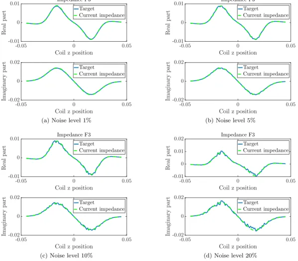
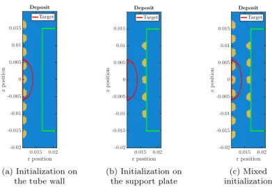
Chapter 4 displays the numerical results for the 2D-axisymmetric algorithm. After some impor-tant remarks on different measures taken to improve the computational time of one iteration, by solving for the scattered field, or re-arranging the assembly operations from one iteration to another, we present some validating numerical results. We intend this chapter to be as thorough possible, by discussing for instance the influence of the initialization on the convergence or that of the various optimization parameters, to use the different observations we make for the 3D algorithm. We as well evaluate the robustness of the method to noise at different steps in the ECT process: uncertainty in the probe position, in the physical parameters, in the impedance signal and in the tube thickness. Though the majority of the tests invert synthetic data, we conclude with the inversion of signals from mock-up situations provided by the power plant operator.

In Chapter 5 we move onto the 3D model. Compared to the 2D-axisymmetric model, new diffi-culties arise from the simulation of electromagnetic waves as they require edge elements, as explained

by [20] and [50], in order to ensure the continuity of tangential components. Under the eddy-current

approximation, the medium conductivity introduces a different behavior between the insulate and the

conductor, as well as differential constraints as explained in [1, Chapter2]. In addition, depending on

the topological nature of the insulate and conductor, should they not be simply connected, additional harmonic fields may need to be computed on each connected component. Different approaches can be

considered to solve the 3D Eddy Current Maxwell equations, for instance with scalar potentials [7].

sim-Contents 5

ply connected insulate domains, in the context of shape reconstruction, the conductive and insulate domains are bound to change over the course of the algorithm. Instead, we choose here the formula-tion with potentials pA, V q defined by µH “ curl A and E “ iωA ` grad V , with the Coulomb gauge

[1, Chapter 6]. Compared to a E-based or H-based formulation, the pA, V q formulation has a better

and simpler structure and requires only assumptions on the connectivity of the whole computation domain (i.e. the union of conductive and insulator parts). Due to the assumed size of the problem to solve, we tackle in this chapter the parallel resolution of the resulting equations. The specificity of the reconstruction algorithm is that generation of impedance signals requires to solve the same equations for different right-hand sides. This motivates a benchmark of four different iterative solvers:

GMRES [65], GCRODR [41], block GMRES [28] and block GCRODR [49]. While GMRES and to

a lesser extent GCRODR are widely used algorithms to solve linear systems, block iterative solvers allows the user to solve blocks of right-hand sides at the same time, which is an interesting feature for our problem. We also discuss in this chapter the numerical consequences of defining the deposit geometry using a Level-Set function in the resolution of Maxwell equations: when interpolated to the computational mesh, the deposit numerical surface becomes strongly non-regular, creating insta-bilities. We look at different strategies to remove such numerical instainsta-bilities. We close the chapter

with the plate modeling, based on impedance boundary conditions derived in [44].

In the last chapter, we derive the 3D reconstruction algorithm. We start from the algorithm

defined in [29, 37] and add a Level-Set framework to it. Numerical experiments are then conducted.

Here we have two different probes available to deposit detection: an axisymmetric probe, SAX, and a

probe made of two rows of coils allocated around the probe axis, SMX (see [51] for more probes used

in ECT). We compare throughout different test configurations the performances of the reconstruction algorithm with the two different probes: computational time, optimal solution, final data fit . . . We also make use of the 2D-axisymmetric reconstruction algorithm on some simple cases to validate the accuracy optimality of the 3D inversion on axisymmetric configurations.

Introduction

L’´electricit´e en France est en grande partie g´en´er´ee (autour de 70% de la production nationale) par l’un

des 56 r´eacteurs nucl´eaires r´epartis dans 18 centrales nucl´eaires. EDF, en tant qu’op´erateur historique

de ces centrales, assure le bon fonctionnement des diff´erentes infrastructures. Le fonctionnement de la

centrale est r´egie par diff´erentes r`eglementations permettant d’´eviter tout incident `a l’origine de fuite

radioactive dans l’environnement. Pour respecter ces normes, chaque centrale est inspect´ee durant ce

que l’on appelle des ”arrˆets de tranche” pendant lesquels la centrale est arrˆet´ee pour pouvoir ´evaluer

la fatigue et l’usure des infrastructures et s’assurer de la sˆuret´e de l’ensemble afin de pouvoir continuer

`

a fonctionner.

(a) Dessin de l’int´erieur d’un g´en´erateur de vapeur

(b) Image du faisceau tubulaire

Figure 0.3: G´en´erateur de vapeur

Cette th`ese se concentre sur l’inspection des g´en´erateurs de vapeur (GV), les ´echangeurs

thermiques de la centrale. Figure0.3exhibe les principales composantes du GV, `a savoir un ensemble

de plus d’un millier de tubes en U (entre 3500 et 5600 tubes selon le mod`ele de centrale pour ˆetre

plus pr´ecis) stabilis´es `a l’aide de plaques entretoises r´eguli`erement espac´ees le long des tuyaux. A

l’int´erieur de ceux-ci circule l’eau chauff´ee par la r´eaction nucl´eaire en amont, tandis qu’`a l’ext´erieur

des tubes circule de l’eau plus froide. Par contact avec les tubes chauff´es, l’eau froide est vaporis´ee

et la vapeur qui en r´esulte est ensuite utilis´ee pour produire de l’´electricit´e `a l’aide d’un couple

turbine/alternateur.

L’usure `a l’int´erieur des GV a plusieurs origines : les hautes conditions de temp´erature/pression `a

l’int´erieur des tubes, l’eau circulant constamment dans et `a l’ext´erieur des tubes, . . . En cons´equence,

diff´erents types de d´efauts peuvent ˆetre observ´es : des fissures dans l’´epaisseur du tube [54], la

formation de d´epˆots conducteurs sur la paroi ext´erieure du tube par agglutination de particules

m´etalliques [60], . . . Nous nous focalisons dans cette th`ese sur la d´etection de ces d´epˆots m´etalliques,

qu’on peut s´eparer en deux familles :

• d´epˆots colmatants, entre le tube et la plaque entretoise (cf Figure0.4),

• d´epˆots d’encrassement, en-dehors de la zone de la plaque. Ces d´epˆots sont en g´en´eral longs

selon la direction du tube et fins sur la direction transverse, du fait de la circulation de l’eau le

long du tube, empˆechant la formation de d´epˆots volumiques.

La d´etection de ces d´epˆots est importante pour s’assurer du bon fonctionnement de la centrale

car ils r´eduisent les transferts thermiques sur la paroi du tube [59], r´eduisant ainsi le rendement

du GV et peuvent ´egalement colmater les trous laissant passer l’eau entre la plaque entretoise et le

tube, cr´eant ainsi des contraintes m´ecaniques suppl´ementaires sur les conduites, acc´el´erant de fait

leur usure. Pour se d´ebarrasser des d´epˆots, un nettoyage chimique est utilis´e par l’op´erateur. Cette

op´eration ´etant coˆuteuse, il a ´et´e convenu qu’au-del`a d’un pourcentage de colmatage du GV d´ecid´e

par des r´eglementations, le processus de nettoyage est enclench´e. Il est donc important de pouvoir

estimer ce pourcentage de colmatage.

Figure 0.4: Dessin d’un d´epˆot colmatant entre la plaque entretoise et le tube (coupe transverse).

Pour diff´erentes raisons (inaccessibilit´e, radioactivit´e des composants, coˆuts ´economiques, . . . ),

une observation directe de l’int´erieur des GV n’est pas permise. Le Contrˆole Non Destructif

(CND) est une approche utilis´ee en industrie pour obtenir de l’information sur l’´etat d’un objet sans

avoir `a l’endommager. Dans le cas pr´esent, le CND constitue une m´ethode indirecte permettant

d’analyser la configuration `a l’int´erieur des GV pour chaque tube sans avoir `a ˆetre physiquement

pr´esent dans le bˆatiment r´eacteur et sans mettre en danger l’engin. Il existe une grande vari´et´e

de m´ethodes `a base de CND pouvant s’appliquer `a un grand nombre de configurations. Parmi ces

m´ethodes, le contrˆole par courants de Foucault (ECT en anglais) constitue une approche adapt´ee

`

a la d´etection de d´epˆots m´etalliques. Un champ ´electromagn´etique alternatif cr´ee sur des surfaces

conductrices des courants de surface appel´es courants de Foucault. La formation de ces courants

est directement li´ee `a la loi de Faraday (`a savoir qu’une variation temporelle du champ magn´etique

induit en retour un champ ´electrique) : sur des mat´eriaux conducteurs, la variation de champ va

cr´eer des courants de surface proportionnels `a la conductivit´e suivant la loi d’Ohm. Par cons´equent,

ces courants vont `a leur tour induire un nouveau champ ´electromagn´etique qui va venir perturber le

champ incident : la m´ethode ECT utilise cette perturbation du champ pour obtenir de l’information

sur l’´etat des parties conductrices du domaine. Pour g´en´erer le champ ´electromagn´etique est utilis´ee

une sonde contenant des bobines soumises `a un courant I. Pour mesurer la perturbation, la sonde

compare le flux `a travers une bobine (r´eceptrice) du champ perturb´e avec celui du champ incident

`

a travers une autre bobine (´emettrice), diff´erente ou non : c’est ce que l’on appelle l’imp´edance.

En pr´esence d’un d´efaut dans les parties conductrices l’imp´edance aura une signature non nulle

con-tenant ainsi des informations sur ledit d´efaut. La m´ethode d’ECT peut s’appliquer `a diff´erentes

probl´ematiques, comme par exemple la d´etection de fissures `a l’int´erieur des GV [51, 40] ou dans

d’autres configurations [31], ou bien coupl´e avec de la thermographie au travers de l’effet Joule [26].

Dans le cas pr´esent, le processus de d´etection choisi est le suivant : apr`es avoir vid´e le GV de

Contents 9

constante : `a des positions donn´ees le long du tube, elle va prendre une mesure, g´en´erant ainsi `a la

fin un signal d’imp´edance. L’analyse du signal ainsi obtenu permet d’obtenir de l’information sur la

forme et la position du d´epˆot. En l’´etat, le traitement des donn´ees se base sur des mod`eles empiriques

´elabor´es `a partir de bases de donn´ees : la phase et l’amplitude du signal sont utilis´ees pour obtenir

de l’information g´en´erale sur l’´epaisseur et la longueur du d´epˆot.

Une telle m´ethode constitue un outil puissant capable d’analyser une grande quantit´e de donn´ees

tout en donnant des informations g´en´erales sur le d´epˆot, ce qui est suffisant pour l’op´erateur pour

d´ecider du d´eclenchement ou non du nettoyage chimique. Cependant dans des configurations plus

complexes, par exemple lorsque le tube a une ´epaisseur l´eg`erement non constante ou pour des formes

de d´epˆots pathologiques, une telle approche peut conduire `a une mauvaise interpr´etation des donn´ees.

Ceci motive la construction d’un autre algorithme de traitement capable de reconstruire pr´ecis´ement

n’importe quelle forme de d´epˆot. Nous nous proposons ici de d´evelopper une approche se basant sur

la mod´elisation des ph´enom`enes physiques li´es au processus et de formuler le probl`eme comme un

probl`eme inverse. L’objectif de cette famille de probl`emes est d’estimer des param`etres y `a partir

de mesures indirectes z li´ees `a la physique du syst`eme et un mod`ele A qui transforme les param`etres y

en mesures z : Apyq “ z. Supposons que A soit connu, il faut ”l’inverser” pour calculer y `a partir de

z. Dans le cas pr´esent, y est la forme du d´epˆot dans le domaine de calcul, z est le signal d’imp´edance

et A contient les ´equations de Maxwell qui permettent de calculer le champ ´electromagn´etique et

donc l’imp´edance. Compar´e `a des m´ethodes empiriques, une telle approche inverse assure une bonne

reconstruction du d´epˆot, au prix d’une plus grande complexit´e et d’une analyse plus lente de part le

calcul de A.

Comme A est connu, il est possible de g´en´erer pour n’importe quelle forme y le signal d’imp´edance

z qui lui correspond. De fait, ”l’inversion” de A peut se formuler comme un probl`eme d’optimisation

de forme o`u la fonctionnelle coˆut est l’´ecart aux moindres carr´es entre le signal d’entr´ee ˜z et le mod`ele

num´erique Apyq. En trouvant la forme y qui minimise la fonctionnelle coˆut, nous avons reconstruit

la solution de notre probl`eme.

L’optimisation de forme est un type de probl`eme d’optimisation qu’il est possible de rencontrer

en m´ecanique solide (par exemple la conception optimale de structures soumises `a des contraintes

m´ecaniques et de volume donn´ees) [24] ou fluide [10]. Elle est ´egalement largement utilis´ee en

´electromagn´etique dans le contexte de probl`emes de diffraction inverse [48,14,38], ou plus pr´ecis´ement

pour l’inspection de mat´eriaux conducteurs `a l’aide de m´ethodes d’ECT comme discut´e dans cette

th`ese. A propos de la reconstruction de forme `a l’aide de courants de Foucault dans les GV, des

travaux pr´eliminaires ont ´et´e conduits par [67,69,68] pour des g´eom´etries 2D-axisym´etriques et par

[29,37] pour des configurations 3D. Ces papiers utilisent une descente de gradient pour r´esoudre le

probl`eme d’optimisation, en consid´erant que la fronti`ere du d´epˆot est l’inconnue `a optimiser : `a chaque

it´eration, la fronti`ere est d´eform´ee par le gradient. Dans cette approche, la forme est explicitement

d´efinie dans le domaine de calcul : cela permet d’avoir une bonne pr´ecision sur la forme du d´epˆot

au prix d’un coˆut de calcul ´elev´e car chaque it´eration n´ecessite la cr´eation d’un nouveau maillage et

d’une re-d´efinition du probl`eme. Le travail expos´e dans cette th`ese consiste en l’int´egration de

fonc-tions Level-Set `a l’algorithme de reconstruction. L’utilisation de telles fonctions en optimisation de

forme s’est r´epandue dans de r´ecents travaux, notamment dans la conception optimale de structures

[66,25], dans les probl`emes de diffraction inverse [48], en tomographie optique [45], ou en m´ecanique

des fluides [56]. La d´eclaration implicite de la forme `a l’aide d’une fonction Level-Set constitue un

outil permettant de mieux g´erer des changements topologiques de la forme comme la fusion ou la

s´eparation en deux composantes connexes. Dans un second temps, cela permet de conserver le mˆeme

domaine de calcul `a chaque it´eration, au prix d’une pr´ecision plus faible sur la forme qui doit ˆetre

interpol´ee.

Nous aimerions maintenant pr´esenter nos contributions au probl`eme de d´etection au travers d’un

rapide r´esum´e du contenu du manuscrit. Apr`es un chapitre introductif d´efinissant les principaux

mots-cl´es de la th`ese, le manuscrit se subdivise en deux parties traitant de la reconstruction de

d´epˆots, d’une part pour des configurations 2D-axisym´etriques et d’autre part pour des configurations

3D g´en´eriques.

Dans le chapitre deux, nous ´elaborons un mod`ele physique pour le domaine 2D-axisym´etrique :

`

le signal d’imp´edance qui en r´esulte. En pr´esence de courants de Foucault, il a ´et´e observ´e que la

variation temporelle du champ ´electrique dans le conducteur est tr`es petite lorsque la pulsation ω du

courant alternatif est relativement faible. Cela conduit `a l’approximation des courants de Foucault

σ " ωε, o`u σ est la conductivit´e du milieu et ε, sa permittivit´e. A partir de cette approximation, nous

restreignons les g´eom´etries `a des surfaces de r´evolution, autrement dit le domaine peut ˆetre g´en´er´e

en faisant tourner une courbe autour d’un axe de rotation. Cela permet, d’apr`es le travail de [19],

de r´eduire le syst`eme `a six inconnues li´e aux ´equations de Maxwell `a un syst`eme `a trois inconnues

d´efini sur un plan 2D. En s’appuyant sur le mod`ele 2D-axisym´etrique d´efini par [69], nous ajoutons au

domaine des caract´eristiques plus complexes pour pouvoir mieux rendre compte de l’int´erieur des GV.

Nous proposons dans ce chapitre de consid´erer les trois composantes suivantes : la plaque entretoise

conductrice pour pouvoir ´etudier la d´etection de d´epˆots colmatants, les d´epˆots fins d’encrassement

en-dehors de la zone de la plaque et une variation fine de l’´epaisseur de tube. Un souci particulier doit

ˆetre apport´e `a la mod´elisation de ces diff´erentes caract´eristiques pour assurer une r´esolution rapide

des ´equations. Par exemple, comme la plaque entretoise est hautement conductrice, du fait de l’effet

d’´epaisseur de peau, le champ ´electromagn´etique va p´en´etrer une tr`es fine ´epaisseur du mat´eriau avant

d’ˆetre totalement dissip´ee. La prise en compte de cette fine variation peut tr`es vite s’av´erer coˆuteuse,

c’est pourquoi nous pr´ef´erons remplacer la plaque par une condition d’imp´edance sur sa fronti`ere.

Cette condition de bord permet d’avoir une mise `a l’´echelle des champs ´electrique et magn´etique

sur la surface, ainsi qu’une meilleure approximation pour prendre en compte des ph´enom`enes de

r´eflexion par des mat´eriaux hautement conducteurs. Ces conditions d’imp´edance constituent en

r´ealit´e une approximation aux premiers ordres de ce qu’on appelle Generalized Impedance Boundary

Conditions. Ces conditions de bord plus g´en´eriques ont ´et´e ´etudi´ees dans deux cas sp´ecifiques, li´es `a la

diffraction d’ondes ´electromagn´etiques : les mat´eriaux hautement conducteurs [44] ou bien les couches

minces recouvrant des mat´eriaux parfaitement conducteurs [3]. Une analyse formelle du probl`eme

de diffraction avec GIBC a ´et´e conduite par [13]. Elles peuvent ˆetre utilis´ees pour des probl`emes de

diffraction inverse [38] pour reconstruire la surface diffractante. Nous adoptons ce mˆeme formalisme

asymptotique pour traiter des couches fines comme la variation fine d’´epaisseur de tube ou bien les

d´epˆots fins d’encrassement. Mailler la g´eom´etrie de ces d´efauts fins pour calculer les champs s’av`ere

tr`es rapidement coˆuteux du fait de leur taille. Nous choisissons ici de les enlever du domaine de calcul

pour les remplacer par des fonctions d’´epaisseur en munissant les interfaces appropri´ees de conditions

d’imp´edance de transmission (ICT en anglais). L’´etude de couches fines de mat´eriaux conducteurs

n’est pas r´ecente, des papiers comme [39] ont d´evelopp´e des mod`eles pour une formulation pH, V q

des ´equations. Plus r´ecemment, les ICT ont ´et´e ´etudi´ees en 2D [57,58] dans un cadre harmonique ou

magneto-quasistatique, ou bien en 3D [62]. L’approche d´evelopp´ee dans ces papiers ressemble `a celle

utilis´ee pour les plaques entretoises : en mettant `a l’´echelle la conductivit´e par rapport `a l’´epaisseur

de la couche, des d´eveloppements asymptotiques des champs dans la couche par rapport `a l’´epaisseur

permettent de construire les conditions de transmission `a appliquer sur les interfaces.

Le troisi`eme chapitre d´eveloppe l’algorithme de reconstruction. Dans [69], le probl`eme d’optimisation

de forme est r´esolu en utilisant une m´ethode de variation de fronti`ere coupl´ee `a une descente de

gra-dient : `a chaque it´eration le gradient est utilis´e pour mettre `a jour la fronti`ere de la forme. Comme

nous l’avons expliqu´e plus haut, comme la forme est explicitement d´efinie dans le domaine de

cal-cul, une modification de la forme n´ecessite de red´efinir le domaine ainsi que les ´equations d’´etat.

Nous proposons dans ce chapitre de d´evelopper un algorithme de reconstruction se basant sur l’usage

des fonctions Level-Set. La diff´erenciation formelle de la fonctionnelle coˆut repose sur les travaux

pr´eliminaires de [24,5]. Les probl`emes inverses sont naturellement mal pos´es au sens de Hadamard :

dans notre cas cela signifie que diff´erentes formes optimales peuvent donner les mˆemes signaux du

fait du nombre limit´e de mesures et ces minimums sont instables par rapport `a une variation fine

des donn´ees. Pour r´esoudre cette contrainte, des r´egularisations peuvent ˆetre ajout´ees au probl`eme

d’optimisation, comme par exemple des contraintes suppl´ementaires pour discriminer certaines

solu-tions, l’utilisation de r´egularisation de Tikhonov, . . . Nous proposons dans cette th`ese d’ajouter une

p´enalisation du p´erim`etre `a la fonction coˆut : l’´etude dans les GV montre que les d´epˆots qui se forment

sur les tubes ont une forme lisse avec peu d’oscillations. En for¸cant la solution `a avoir un p´erim`etre

minimal, nous esp´erons forcer l’unicit´e de la forme optimale. En plus de la reconstruction de la forme

du d´epˆot, nous ajoutons au probl`eme d’optimisation deux variables suppl´ementaires correspondant `a

l’´epaisseur des d´epˆots fins d’encrassement ainsi que la variation d’´epaisseur de tube. Dans un second

temps nous pr´esentons l’algorithme d’optimisation par rapport `a ces deux inconnues. Enfin, dans les

Contents 11

ph´enom`ene complexe `a l’origine de leur formation. Par cons´equent nous ajoutons l’option de pouvoir

reconstruire ces propri´et´es physiques, en les supposant constantes dans le mat´eriau.

Le chapitre quatre pr´esente les r´esultats num´eriques pour l’algorithme 2D. Apr`es d’importantes

remarques sur les diff´erentes mesures que nous avons prises pour am´eliorer le temps de calcul

d’une it´eration d’inversion, en calculant le champ diffract´e ou bien en r´earrangeant les op´erations

d’assemblage d’une it´eration `a l’autre, nous pr´esentons diff´erents tests permettant de valider l’algorithme.

Ce chapitre se veut aussi exhaustif que possible, par exemple au travers de discussions sur le choix

de l’initialisation, ou bien des diff´erents param`etres de r´egularisation dans le but d’utiliser ces

ob-servations pour l’algorithme 3D. Nous ´etudions ´egalement la robustesse de la m´ethode `a diff´erents

degr´es d’impr´ecision dans le processus de d´etection : incertitude dans la position de sonde, dans les

param`etres physiques, dans le signal d’imp´edance ou dans l’´epaisseur de tube. Bien que la plupart

des tests soient construits sur des donn´ees artificielles, nous concluons avec l’inversion de signaux

provenant de maquettes g´en´er´es par l’op´erateur des centrales nucl´eaires.

Dans le chapitre 5 nous ´etudions le mod`ele 3D. Compar´e au mod`ele 2D-axisym´etrique, de

nou-velles difficult´es dans la mod´elisation apparaissent du fait de la simulation d’ondes ´electromagn´etiques

qui requi`erent l’utilisation d’´el´ements d’arrˆete comme expliqu´e par [20] et [50], pour assurer la

conti-nuit´e des composantes tangentielles. Sous l’approximation des courants de Foucault, la conductivit´e

du milieu introduit diff´erents comportements entre le milieu isolant et le milieu conducteur, de mˆeme

que des contraintes diff´erentielles comme expliqu´e dans [1, Chapitre 2]. De plus, selon la nature

topologique des deux milieux, `a savoir selon qu’ils soient simplement connexes ou pas, il faudrait

ajouter le calcul de champs harmoniques sur les diff´erentes composantes connexes. Diff´erentes

ap-proches peuvent ˆetre consid´er´ees pour r´esoudre les ´equations de Maxwell, par exemple avec des

potentiels scalaires [7]. Bien que cette formulation permette de r´eduire le coˆut m´emoire pour la

discr´etisation num´erique du probl`eme pour des domaines simplement connexes, dans le contexte de la

reconstruction de forme, les domaines conducteur et isolant sont amen´es `a changer selon les it´erations.

De fait nous proposons ici de formuler les ´equations de Maxwell `a partir des potentiels pA, V q d´efinis

par µH “ curl A et E “ iωA ` grad V , munis de la jauge de Coulomb [1, Chapter 6]. Compar´e `a

une formulation en le champ ´electrique E ou magn´etique H, la formulation en potentiels pA, V q a une

meilleure structure, plus simple et ne requiert que des pr´esuppos´es sur la connectivit´e du domaine

global. De part la taille attendue du domaine `a r´esoudre, nous traitons ´egalement dans ce chapitre la

parall´elisation des ´equations. La sp´ecificit´e de l’algorithme de reconstruction est que la g´en´eration des

signaux d’imp´edance n´ecessite de r´esoudre les mˆeme ´equations pour diff´erents seconds membres. Cela

motive une comparaison de quatre solveurs it´eratifs : GMRES [65], GCRODR [41], block GMRES

[28] et block GCRODR [49]. Tandis que GMRES et dans une moindre mesure GCRODR sont des

algorithmes tr`es r´epandus pour la r´esolution de syst`emes lin´eaires, des solveurs par blocs permettent

de r´esoudre des blocs de seconds membres en mˆeme temps, caract´eristique int´eressante pour notre

probl`eme. Nous discutons ´egalement dans ce chapitre des cons´equences num´eriques de la d´efinition

implicite de la g´eom´etrie du d´epˆot `a l’aide de fonctions Level-Set dans la r´esolution des ´equations

de Maxwell : une fois interpol´ee sur le maillage de calcul, la fronti`ere num´erique du d´epˆot devient

tr`es irr´eguli`ere, cr´eant des instabilit´es. Nous regardons diff´erentes strat´egies permettant d’enlever

ces instabilit´es num´eriques. Nous terminons ce chapitre par l’´elaboration du mod`ele pour la plaque

entretoise, bas´e sur les conditions d’imp´edance d´efinies dans [44].

Dans le dernier chapitre, nous d´eveloppons l’algorithme de reconstruction 3D. Nous nous appuyons

dans un premier temps sur l’algorithme d´efini par [29, 37] pour ajouter ensuite la mod´elisation

du d´epˆot par fonction Level-Set. Des exp´erimentations num´eriques sont ensuite conduites. Dans

ce chapitre, nous pouvons utiliser deux sondes diff´erentes pour d´etecter le d´epˆot : une sonde

ax-isym´etrique, SAX, et une sonde faite de deux rang´ees de bobines autour de l’axe de la sonde, SMX

(voir [51] pour plus d’exemples de sondes utilis´ees pour le CND dans les GV). Nous comparons ainsi

au travers de diff´erents cas tests les performances de l’algorithme de reconstruction avec les deux

sondes : le temps de calcul, la solution optimale, l’attache aux donn´ees finale, . . . Nous nous

ser-vons ´egalement de l’algorithme 2D-axisym´etrique sur des cas simples axisym´etriques pour valider la

Chapter 1

Eddy-Current Testing in Steam

Generators

Contents

1.1 Industrial Overview . . . 14

1.2 Eddy Current Approximation . . . 17

1.2.1 Maxwell Equations . . . 17

1.2.2 Eddy Currents . . . 19

1.2.3 pA, VCq-formulation . . . 21

1.2.4 Numerical computation . . . 23

1.3 Deposit detection in Steam Generators . . . 24

1.3.1 Model definition . . . 24

1.3.2 2D axisymmetric approximation . . . 27

1.3.3 Impedance Signal . . . 28

1.4 Inverse problems . . . 31

Non-Destructive Testing, or NDT, is a powerful tool used in science and in industries to assess the properties of a material without altering or damaging it. Depending on the nature of the system tested, a wide variety of methods can be used, ranging from acoustic emission to detect cracks or leaks to radiographic testing for airport security for instance.

In this thesis, we consider one type of NDT called Eddy Current Testing, or ECT. This method exploits a well-known electromagnetic phenomenon: in presence of an alternating magnetic induction B, small surface currents appear on a conductive material. These currents are called eddy current.

They are a consequence of Faraday’s law of induction, as illustrated by Figure 1.1: a variation of

the magnetic flux, manifested by a tilde, creates a circular electric field E that induces in return a current I.

In presence of a conductive defect, the circulation of the eddy currents is disturbed, yielding a perturbation of the magnetic induction. ECT makes use of this distortion to obtain information on the state of the system, that is to say, presence of cracks, defects, ... The perturbation is measured using the flow of the magnetic induction through a coil, called impedance.

In this thesis, we consider the use of ECT for the inspection of nuclear power plants, specifically inside steam generators, noted SG, to detect conductive deposits on tubes. As they may alter the yield of the power plant, the operator wants to assess the proportion of deposits inside the machine, in order to activate chemical cleaning that will remove the impurities.

In this introductive chapter, we first present the industrial context underlying this work. In a second part, after introducing Maxwell equations, we specify the equations in presence of eddy currents for which the approximation σ " ωε is verified, where σ is the conductivity and ε, the permittivity of the medium, and ω, the pulsation. The last part focuses on the application of the eddy current equations to ECT in Steam Generators.

1.1

Industrial Overview

Nuclear power plants are thermal power plants using nuclear fuel to produce electricity. Their oper-ation is the following: water is used to transfer heat generated by a heating source, here the nuclear reaction. It then vaporizes water which eventually transforms the thermal energy to a mechanic

energy, converted at the end to an electric energy. Figure 1.2displays here the main features of a

Pressurized Water Reactor, noted PWR.

Figure 1.2: Schematic operation of a nuclear power plant. Source : IRSN.

At the heart of the power plant is the nuclear reactor: radioactive fuel assemblies are plunged inside a nuclear vessel. When the fuel unstable nuclei are hit by neutrons, they split into more stable nuclei and two/three neutrons, that will then hit other unstable nuclei. By chain reaction, the nuclear reaction continues. Different levers exist to control its intensity: for instance, adjusting how deep the modules are plunged in the nuclear vessel, or using bore atoms in the water to absorb a portion of the neutrons. This helps the operator control the power produced to meet the fluctuations in the demand in electricity. The energy produced by the fission is used to heat water, maintained in liquid phase using a pressuriser, flowing inside the primary loop. The heat transported by the water is then

1.1. Industrial Overview 15

used to vaporize colder water inside the steam generator. All these structures are enclosed inside the reactor building, whose main purpose is to stop potential radioactivity leak from pouring in the environnement.

The vapor water coming from the steam generator is taken to a turbine, coupled with an alternator to produce electricity. The vapor is then condensed using a condenser: the resulting liquid water flows back to the steam generator. The liquid/vapor water form the secondary loop.

The condenser that cools the vapor uses cold water from different sources: the sea, the ocean, the river coupled or not with cooling towers. That forms the cooling loop.

Figure 1.3: Sketch of the interior of a steam generator

The focus of this work is the inspection of the steam generator, where water is vaporized.

Fig-ure1.3shows the characteristics of the device: it is composed of a cluster of more than a thousand

U-shaped tubes where hot water from the primary loop flows. These tubes are plunged inside cooler water from the secondary loop. By contact with the tubes, colder water vaporizes and flows upwards, towards the turbine.

Due to their geometry (diameter ! height), the tubes are maintained still using support plates evenly spaced in the tube direction, to limit the tube oscillation induced by the water flowing inside. In the Steam Generators considered, these plates, made out of a highly conductive material, are drilled

with quatrofoil holes to let both the tube and the water come through it, as shown on Figure2.2.

Figure 1.4: Sketch of a plugging deposit between the plate and the tube (cross section). Over the course of the power plant operation, different deteriorations can be observed inside the steam generator, like formation of cracks for instance. We consider here corrosion phenomena occuring

in the secondary loop: soluble matter or particles like iron oxyde or magnetite Fe3O4form inside the

steam generator, forming eventually deposits on the tube exterior. These conductive deposits may be of two types:

• plugging, between the tube and the support plate (cf Figure2.2),

• clogging, outside the plate area. These deposits are usually long in the tube axis direction and thin in the transverse direction.

For more details on the formation of plugging and clogging deposit, we advise the reader to read

the theses [60] and [59].

For the power plant operator, these deposits are unwanted as they deteriorate heat transfer on the tube exterior and alter the flow of the water from the secondary loop. They also harm security of the device, for instance the integrity of the tubes or the equipment of the Steam Generator, should the proportion of clogging deposits be high enough. To remove them, a cleaning process using chemicals can be done. However, the cleaning process is highly costly for the company, for various reasons. Detection of such structures then is more than important for the operator as it gives information of the proportion of deposits: should it excess a chosen value, the cleaning is activated. A natural solution for the detection would be to physically check inside the steam generator, which is only partially possible using a robot equipped with a camera. The device can only access the top (and sometimes the middle) tube support plate and can reach only one of the quadrofoil holes with limited

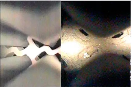
precision. Figure 1.5displays the type of picture that can be taken from the top: as evidenced by

the pictures, processing the image leads to incomplete information about the whole device state. Direct observation of the tubes to obtain precise information on the presence of deposits is therefore prohibited: this calls for Non Destructive Testing.

Figure 1.5: Example of picture taken from the top of the tubes. Left: no plugging deposit, right: partial plug.

Non Destructive Testing (NDT) provides tools that does not rely on direct observation and at the same time does not harm the inspected structure. It covers a wide variety of methods such as eddy current, magnetic particle, liquid penetrant, radiographic, ultrasonic, visual testing, ... As the support plate, deposit and tube inside the Steam Generator are conductive, Eddy Current Testing (ECT) constitutes a suitable approach. The detection process using ECT is the following. After emptying the device from the water, probes are inserted from one end of each tube, to the other end. By pulling them out at a constant speed, the operator is able to make measurements at regular positions alongside the tube.

The probes are composed of a given set of coils: when a coil, called the emitter, is subjected to a current I, it produces an incident electromagnetic field. On the surface of conductive materials, eddy currents generate an other electromagnetic field, disturbing the former. An other coil, called the receiver, then measures the flow of the distorted field and compares it to that of the incident field:

1.2. Eddy Current Approximation 17

the difference of flows is called impedance. It constitutes the data to invert as it contains information on the deposit.

Different probes can be used in the ECT process, to obtain different information on the configu-ration. In this work, we consider two of them : the SAX probe and the SMX probe. The SAX probe is made out of two axial coils placed in the tube direction, whereas the SMX probe is composed of

two rows of coils, placed at different azimuthal coordinates, as displayed on Figure1.6.

Figure 1.6: Picture of a SMX probe.

As the tube and SAX probe coils share the same axis, this device provides information on the deposit that is averaged on the azimuthal direction whereas the SMX probe gives different information on this direction.

1.2

Eddy Current Approximation

Before getting into the specifics of the formation of eddy currents, let us first present the generic Maxwell equations, then focus on the time-harmonic formulation of these equations.

1.2.1

Maxwell Equations

Maxwell’s four equations describe the electric and magnetic inductions arising from distributions of electric charges and currents, and how those fields change in time. Even though they are now known as Maxwell equations, they originally were four different laws observed and formulated by different scientists that Maxwell had the idea to combine in order to describe electromagnetic phenomena. It can be formulated either locally or integrally, the former being easy to use for calculations and the latter to understand the physical justifications of the formulae.

Let us introduce the fields E px, tq and Bpx, tq, respectively the electric field and magnetic induction depending on the spatial variable x and the time t. We consider their propagation inside vacuum,

of constant permittivity and permeability εv and µv, with a current density J px, tq and a charge

density ρpx, tq. The first law links the flux of E through an enclosed surface S to the total charge Q inside the volume V delimited by S:

£ S E ¨ dS “ Q ε0 “ 1 ε0 ¡ V ρ dx : Gauss’s law (1.1)

The second law is analogous to the previous as it gives information on the flow of B through an enclosed surface S and is a consequence of the experimental fact that magnetic charges do not exist:

£

S

B ¨ dS “ 0 : Gauss’s law for magnetism (1.2)

The two remaining laws link time-variation of the flow of the fields through an open surface Σ to their circulation on C, the closed curve enclosing Σ:

¿ C E ¨ dl “ ´d dt ij Σ

B ¨ dS : Faraday’s law of induction (1.3)

¿ C B ¨ dl “ µ0pI ` IDq “µ0 ¨ ˝ ij Σ J ¨ dS ` ε0 d dt ij Σ E ¨ dS ˛

‚ : Maxwell-Amp`ere’s law (1.4)

where I “ť_ΣJ ¨ dS the current and ID“ ε0_dtd

ť

ΣE ¨ dS, the displacement currents.

Originally, Faraday’s law was formulated to model the creation of an electromotive force on a conductive material by the time variation of the magnetic flux. It was rewritten in the present form by Maxwell to link to the electric field.

Amp`ere’s law explains that the magnetic circulation on a closed curve is equal to the enclosed

currents. In its first form, only the currents from the density where taken into account, unable to model some physical phenomena. Maxwell added the displacement currents which symbolizes the current created by the displacement of charged particles.

Using Gauss-divergence and Stokes theorems, these laws are re-written in a local form to become the Maxwell equations:

∇ ¨ E “ ρ

ε0

: Maxwell-Gauss equation (1.5a)

∇ ¨ B “ 0 : Maxwell-Thomson equation (1.5b) ∇ ˆ E “ ´BB Bt : Maxwell-Faraday equation (1.5c) ∇ ˆ B “ µ0 ˆ J ` ε0 BE Bt ˙

: Maxwell-Amp`ere equation (1.5d)

Note that by taking the divergence of (1.5d), using (1.5a) and the fact that ∇ ˆ p∇ ¨ q “ 0, we

derive the equation for charge conservation: Bρ

Bt ` ∇ ¨ J “ 0 : Charge conservation (1.6)

The equation guarantees that the total electric charge of an isolated system never changes, or rather, that a change in the charge inside a volume V is equal to the difference between the current flow going in and out of the volume.

To extend the model to more complex medium, where µpx, tq and εpx, tq are non constant, the equations need to be slightly modified. Introducing the electric induction Dpx, tq and the magnetic field Hpx, tq, the Maxwell equations become:

∇ ¨ D “ ρ : Maxwell-Gauss equation (1.7a)

∇ ¨ B “ 0 : Maxwell-Thomson equation (1.7b) ∇ ˆ E “ ´BB Bt : Maxwell-Faraday equation (1.7c) ∇ ˆ H “ ˆ J `BD Bt ˙

: Maxwell-Amp`ere equation (1.7d)

In most scientific problems, µ and ε are time independent symmetric positive definite matrices and D and B depend linearly on respectively on E and H :

D “ εE, B “ µH

In the present case, we consider isotropic non-homogeneous media, where µ and ε are piecewise constant. In the following, we focus on the study of a sub-problem that are time-harmonic Maxwell equations: probes used by the operator use an alternating current to induce alternating fields where

1.2. Eddy Current Approximation 19

time-dependance is of the form e´iωt_{, ω being the pulsation of the signal. Note that the definition}

time-harmonic fields might be the conjugate in some papers, slightly changing the equations. The alternating current density J is then denoted:

J px, tq “ Re“Jpxqe´iωt‰

where J is a complex-valued vector containing the amplitude and phase of the signal. After a

transient state, it is proven that the different field have the same alternating behaviour, with the same pulsation ω:

Dpx, tq “ Re“Dpxqe´iωt_{‰ , Epx, tq “ Re “Epxqe}´iωt‰

Bpx, tq “ Re“Bpxqe´iωt_{‰ , Hpx, tq “ Re “Hpxqe}´iωt‰

where D, E, B and H are complex-valued vectors. From that we derive the time-harmonic Maxwell equations:

∇ ˆ E ´ iωµH “ 0 (1.8a)

∇ ˆ H ` iωεE “ J (1.8b)

Maxwell-Thomson equation is dropped as it can be obtained by taking the divergence of (1.8a). The

charge distribution ρ is obtained using Maxwell-Gauss equation ρpx, tq “ ∇ ¨ pRerεpxqEpxqe´iωt_sq.

These three equations constitute the starting point of this work.

1.2.2

Eddy Currents

This subsection is based on [1, Chapter 1].

Consider here a generic domain Ω decomposed between a conductive, ΩC, and non-conductive

subdomain, ΩI:“ ΩzΩC. We assume ΩC is strictly included in Ω, that is to say ΩC Ă Ω. Note that

for the configuration inside Steam Generators, BΩCX BΩ ‰ H. Nonetheless, the results displayed

hereafter can be extended for such domains. Let Γ :“ BΩIX BΩC be the boundary between the two

subdomains. We suppose the conductor is not simply connected and write the connected components

ΩCi, i P 1 . . . pΓ: ΩC “

ŤpΓ

i“0ΩCi. Let σpxq be the medium conductivity, by definition null inside ΩI.

Faraday’s law explains that time-variation of the magnetic field induces an electric field: on

conductive materials, that generates small surface currents Jedefined by:

Je“ σE : Ohm’s law

In consequence, time-harmonic Maxwell-Amp`ere becomes:

∇ ˆ H ` piωε ´ σqE “ J (1.9)

Due to the σE term, (1.8a) and (1.9) requires to impose div J “ 0 in the insulator, for compatibility

purposes. Remark it is equivalent to say that there are no charges in the insulator. In the conductor, the charge distribution is defined by:

ρpx, tq “ ∇ ¨ pRerεpxqEpxqe´iωt

sq, in ΩC

Eddy currents have different industrial applications: as they induce a perturbation in the elec-tromagnetic field which can be used to detect abnormalities in materials, through Eddy Current Testing. A other well-known consequence of Ohm’s law is power loss due to electric heating: the passage of electric current inside a conductor produces heat according to Joule’s law. Let P be the heat generated by the conductor, then:

P “ σ´1_J

e¨ Je : Joule’s law

The energy loss created by Joule’s law poses many issues, for instance in power stations as the current flowing inside conductive wires loses its energy, decreasing the performances. However it has