Morphogenesis without central control - case studies in social insect nest construction

(1)

HAL Id: tel-03078918

https://hal.archives-ouvertes.fr/tel-03078918

Submitted on 16 Dec 2020

HAL is a multi-disciplinary open access archive for the deposit and dissemination of sci-entific research documents, whether they are pub-lished or not. The documents may come from teaching and research institutions in France or

L’archive ouverte pluridisciplinaire HAL, est destinée au dépôt et à la diffusion de documents scientifiques de niveau recherche, publiés ou non, émanant des établissements d’enseignement et de recherche français ou étrangers, des laboratoires

Morphogenesis without central control - case studies in

social insect nest construction

Christian Jost

To cite this version:

Christian Jost. Morphogenesis without central control - case studies in social insect nest construction. Quantitative Methods [q-bio.QM]. Université Toulouse 3, Paul Sabatier, 2015. �tel-03078918�

(2)

M ´

EMOIRE

en vue de l’obtention de

l’habilitation `a diriger des recherches (HDR)

Ecole Doctorale Sciences Ecologiques, Vétérinaires, Agronomies, Bioingénieries de l’Université de Toulouse

Spécialité: Ecologie, Biodiversité et Evolution

pr´esent´e par

Christian JOST

sous la direction de Guy THERAULAZ

Morphogenesis without central control - case studies in social insect nest construction

(written in english/r´edig´e en anglais)

Manuscrit version finale, d´ecembre 2015

Soutenue le 11/12/2015 devant le jury compos´e de:

Rapporteur M. Flavio ROCES, University of W¨urzburg, Germany Rapporteur M. Johan VAN DE KOPPEL, NIOZ Yerseke, Netherlands Rapporteur M. Fran¸cois GRANER, Universit´e Paris 7, France

Examinateur M. Jean-Baptiste FERDY,

U. Fédérale de Toulouse — Midi-Pyrénées

Directeur M. Guy THERAULAZ

(3)

(4)

Preface

The present document was written with a simple goal in mind: allow me to defend my ha-bilitation at the University of Toulouse, France. For those not familiar with the concept of “habilitation”: according to the guidelines of the aforementioned University, a habilitation (or “HDR: Habilitation à Diriger des Recherches”)sanctionne la reconnaissance d’un haut niveau scientifique, le caractère original d’une démarche, la maˆıtrise d’une stratégie de recherche dans un domaine large et la capacité à encadrer de jeunes chercheurs (arrêté du 23 novembre 1988, modifié par les arrêtés des 13 février 1992 et 13 juillet 1995, interprété par les circulaires des 5 janvier 1989 et 16 novembre 1992). As you probably guess, it is quite an important document in the french academic system, not least because it will allow me to supervise a PhD student on my own. With this document, I have to convince three referees and a jury that I

• can work at a high scientific level,

• develop my own ideas,

• master a scientific strategy in an extended domain, and

• that I am capable to supervise young scientists.

This document is therefore often written in the first person. But please keep in mind that I worked in a team and that the presented work is mostly teamwork, with influences from everybody with whom I discussed or worked during the last 20 years. I apologize in advance if the value of these influences has been diluted by this emphasis on the first person, please also take a look at the co-author list in the cited papers to get a more complete picture.

Besides this official and target oriented character, I nevertheless hope that the present doc-ument will be of some interest to everybody who is interested in the study of complex biological systems. I will present case studies that combine experimental with theoretical approaches in order to understand the underlying mechanisms of morphogenetic processes in a large sense: from the aggregation of individuals over the aggregation of objects to the collaborative con-struction of a social insect nest. I also hope that it will appeal to a wide interdisciplinary audience, covering biologists, physicists and mathematicians. I have myself started my career with a Masters in Applied Mathematics (Jost, 1993) at the University of Z¨urich, Switzerland, while doing in parallel a Bachelors degree in Biology. Both interests merged during my PhD in ecology (Jost,1998) at the Institut national agronomique Paris-Grignon (supervised by Roger Arditi), where I explored what time series data of prey and predator abundances can tell us about the underlying predator-prey interaction (and, without having ever had any formal course on statistical inference, had to learn on the fly the statistical approaches to model selection). This PhD taught me, amongst other things, that if we only have data of the final result in a

(7)

biological process (here predator-prey abundances, measured several times to catch the dynam-ics), we have only limited statistical power to infer something on the underlying processes (here prey growth, predation, predator growth). I was therefore lucky to get my job here in Toulouse, where the goal was exactly to identify the underlying processes on the individual level that let emerge some intriguing behavior on the collective level. Lucky in two ways, actually: I got the occasion to design and perform my own experiments (easier said than done, the biologists in the lab often sadly shook their heads), and I found colleagues in statistical physics that taught me a modeling approach to understand collective behavior as emerging from the underlying individual behavior. They also taught me that parameter estimation from experimental data is not only a statistical/numerical problem, but that thoughtful modeling combined with sim-ulation (Monte Carlo) can often work wonders. This habilitation is therefore also the story of my scientific journey here in Toulouse, combining mathematics, physics, computer science and biology in order to advance our understanding of pattern formation in social insects.

This document would not have been possible without the enthusiastic participation of many students. I would not want to miss the freshness and (sometimes naive) scientific curiosity of Bachelor level students: I usually set them to work on very precise questions for which I more or less already know the result, but they often surprised me by developing their report beyond my expectations or by insisting on questions that I considered initially to be of less importance but that turned out to shed new light on the studied topic (B-R Bengoudifa, A Guérécheau, N Hurard, B Piccinini, M Schwalm, A Solacroup, V Rossi). Master students in their first year (M1) played an important role because the evaluation of their internship focusses on the research approach and how they develop it, not on the results themselves: it is therefore possible to let them work on speculative questions, their supervision just requires frequent discussions with them and a close look at what they are actually doing in order to refine the methods and identify the results that merit to be further pursued (G Talbot, J Champeau, S de Mendon¸ca, V Loisel, S Causse, D Fouquet, T Robert, L Chauvet, S Faber, C Bonnand, N Boulic, A Uhart, A Pessato, R Runghen). Master students in their 2nd year (formerly called DEA, now simply M2) require a similar supervision, but I try to set them on questions for which I expect publishable results (M Challet, J Verret, S Garnier, E Casellas, J Olivera, M Keromest, V Loisel, D Fouquet, C Péchabadens). Finally, supervising all these students, in particular teaching them the necessary methods and techniques to become operational, was largely facilitated by the active help of the PhD students I co-supervised (M Challet, C Sbai). Working with PhD students is more like a scientific cooperation than student supervision. The hard work is to find a promising subject and how to attack it, the day to day supervision then mostly consists in discussing intermediate results, explore alternative explanations and refine the methods and techniques in order to best anticipate all possible critics and objections of future anonymous referees. The goal is to advance our understanding of the subject and to accompany the PhD student how to achieve that – this type of cooperation is largely based on trust.

Having said all this I just hope that you will enjoy reading part or all of this document. Thanks in advance for your interest.

(8)

Chapter 2

Introduction

“All models are wrong - but some models are useful” Box(1976)

In the title I use the word morphogenesis rather than the more generalpattern formation: what do I mean by this? Wikipedia definesmorphogenesisas “the biological process that causes an organism to develop its shape”. This definition seems to restrict this term to the growth of a single organism (and many authors use this restricted view). However, in biology we also have the concept ofextended phenotype(popularized byDawkins 1982) where an organism develops other things than shape, in particular behavior. By this behavior it also changes its environment and can create patterns in this environment (a bird building its nest, a beaver constructing a dam, ...). Morphogenesis can therefore also be the process how an organism creates patterns in its environment, this is still a biological process. Turner (2002) in his book The extended organism took this concept a step further by treating the resulting pattern as an organism in itself and emphasizing the physiology of such animal built structures (thus resembling even more the wikipedia definition of morphogenesis). The book cover shows a termite mound, illustrating Turner’s preferred model organism. But other social insects such as ants, wasps or bees also construct nests that don’t shy a comparison with termite mounds. With social insects we have arrived in the field of collective animal behaviors (Sumpter, 2010) or, more general, in group living animals (Krause and Ruxton,2002). My research during the last 14 years has been about understanding how animals collectively create patterns, be it a simple aggregation of individuals (as in cockroaches, Jeanson et al. 2005), the aggregation of objects (as corpse clustering in ants,Theraulaz et al. 2002), or the aggregation of soil pellets to construct a shelter (as in ants, Franks et al. 1992, or in termites, Bruinsma 1979). I consider all such pattern formation processes as morphogenetic processes, and my goal was and is to understand the underlying behavioral mechanisms that coordinate the animal’s behavior in their group.

2.1 Mechanisms of morphogenesis

How are these patterns created? There might be somewhere in the animal a map or a plan of the pattern to be built, the animal just following this plan in order to converge towards the final pattern. This plan might be a genetic program that triggers a sequential order of behaviors that lead to the pattern. The problem with this concept alone is the amount of information that would have to be encoded for such a plan. Even if this were feasible, many animal structures are built collectively: in this case the animal not only needs the sequential program how to build, it also needs the cognitive capacities to assess the state of the structure in order to continue its construction after some coworker has worked on it. In short, the notion

(9)

of a map or plan seems rather complicated to get to work, it is therefore rarely invoked as an explanation for the observed morphogenesis (but see also nest construction in the solitary paper wasp Paralastor sp – Smith 1978; Downing and Jeanne 1988). A second explanation might be that the pattern already exists as a template, though not visible to our eyes. You surely remember the physics experiment in college where iron filings are spread randomly on a sheet of paper above a magnet: when vibrating the paper gently the iron filings become ordered and reveal the form of the magnetic field created by the magnet and that has been there all the time, even if we did not see it. Such patterns can also exist in biological systems as spatial heterogeneities: a humid spot in the soil which will be excavated by ants and form the nest cavity, a temperature or humidity gradient along which the nest is excavated and that serves to raise eggs, pupae or larvae at the right conditions (Brian, 1983; Thom´e,1972). Sometimes the template is created by a single individual as in the case of the Macrotermes subhyalinus queen which emanates constantly a pheromone whose concentration decreases with increasing distance from the queen: it is this concentration that lets workers construct a shelter chamber adapted to the queen’s size (Bruinsma,1979;Ladley and Bullock,2005). This template mechanism also solves the coordination problem between different workers, they are all guided by the template independently of the other worker’s activity. However, a template alone is a limited solution because it must pre-exist somehow. It is also only a partial solution in the case of the termite queen and nuptial chamber construction: as the shelter walls rise, the pheromone concentrations inside will change, thus changing the template. How do the workers maintain the right distance from the queen? This is where an additional concept, self-organization (Camazine

et al.,2001) or stigmergy (Grass´e,1959,1967;Theraulaz and Bonabeau,1999), becomes handy.

Much has already been said about stigmergy: here I will consider it simply as a predecessor of self-organization (SO) and concentrate on the latter. Camazine et al.(2001) define SO as:

Self-organization is a process in which pattern at the global level of a system emerges solely from numerous interactions among the lower-level components of the system. Moreover, the rules specifying interactions among the system’s components are executed using only local information, without reference to the global pattern.

This is a rather wide definition, its key components are only

• dynamical system: a pattern emerges as the result of a dynamic process,

• two or more scales of interest: there are at least two levels in the system (global and lower in the definition, or collective and individual in the examples treated here),

• no global information available to lower level components: the rules guiding the interac-tions between the lower level components (and their environment) only depend on local information (each individual has a limited perception, not extending to the global level, and its behavior is driven by this local information).

Several ingredients of SO are implicitly following from this definition (Bonabeau et al.,1997): • there must be some positive feedback that amplifies small fluctuations (the origin of these

fluctuations can be the result of a random or non-random process) in an out-of-equilibrium system,

• there must also be some negative feedback that finally controls this amplification and helps to stabilize the emerging pattern (forcing it to a stationary state or new equilibrium) The fact that both ingredients exist implies that the dynamical system cannot be linear (if a reader wants a technical definition of a linear or non-linear dynamical system I warmly recom-mend to read the introduction in the habilitation ofGautrais 2015). Other ingredients are less obvious but have been found in all such non-linear dynamical systems:

(10)

• several stable states can co-exist, that is the system can converge to different stationary states as a function of initial conditions and random fluctuations,

• there is always some so-called bifurcation parameter, that is a variable in the system that, if changed, let the pattern on the global level emerge or not.

The last few lines have become rather technical, let’s illustrate them with the termite queen chamber construction. The emerging pattern is the queen chamber, while the local interaction is termite construction activity based on local queen pheromone concentration (template) and, in addition, current theory postulates also mixing of the pellets with some construction pheromone that stimulates further pellet deposits. Actually, when Bruinsma (1979) put an unprotected queen in an arena with soil and termite workers, these workers didn’t build directly a wall around the queen as the template mechanism would suggest, but started by building evenly spaced pillars at the right distance around the queen. These pillars are assumed to be the result of a positive feedback: termites mix pellets with saliva and probably with some pheromone (different from the queen pheromone) before depositing the pellet1. Another pellet transporting termite can sense this local pheromone and its rate to deposit its pellet increases with the sensed construction pheromone concentration. This is the positive feedback. The rising pillars still let the queen pheromone diffuse quite freely around them, thus maintaining the required concentration template. This first phase therefore replaces the pheromone template by a pillar template. Once the pillars are sufficiently high the termites start to fill the space between them from the bottom up, thus building the wall. The negative feedback is simply the completeness of the shelter: once the shelter is finished there are no more pillars with empty space between them (except the entrance hole, see Ladley and Bullock 2005for a possible explanation): with no place where to put new pellets the termite construction activity ebbs out. There are no multiple stable states in this system since there is only one queen, but we will see them in later examples. However, there is a bifurcation parameter: worker density. If the worker density is too low the positive feedback weakens because pheromone evaporates more quickly than new transporting termites arriving at the construction site: no pillars will rise.

As this example shows, morphogenesis is rarely the result of a single mechanism. Here, a template mechanism works hand in hand with SO to let the queen chamber emerge. However, when SO was suggested as an important mechanism in biological pattern formation, the first experimental validations did their best to eliminate explanations other than SO simply to make sure SO was the only possible explanation for the observed patterns (eg. Franks et al. 1992;

Theraulaz et al. 2002;Jeanson et al. 2005). This emphasis on “its only SO” led to some

“accu-sations” that protagonists of SO were too narrow minded and didn’t see beyond SO. I think this debate has now ebbed out: SO does not exclude inter individual variability or even leadership. Inter individual variability can even play a crucial role in a SO process (see review inJeanson

and Weidenm¨uller 2014), such as thermoregulation in honey bees (Jones et al., 2004) where

polyandric colonies have a more stable temperature than monoandric colonies. Leadership in itself is a debated concept (King, 2010; Bourjade et al., 2015), but recent research has shown that its mechanistic origins are diverse and include SO (Petit and Bon, 2010) combined with evolutionary processes (Conradt and Roper, 2010). Gautrais (2010) showed that leadership can result from a combination of inter individual variability and SO, with a continuum from distributed leadership to “despotic” leadership according to certain individual behavioral pa-rameters. Coming back to morphogenesis, SO not only interacts with templates, SO can even generate dynamic templates that play a crucial role in the emerging structure (Jost et al.,2007;

1

Note that the described mechanism hasn’t been experimentally verified in all detail and is currently again under discussion (Petersen et al.,2015). This means that the story told above may have to be refined in the future

(11)

Weitz,2012). A current challenge in morphogenesis is therefore to mount experimental systems where several mechanisms are at work in order to understand their interplay (eg. Jost et al. 2007), preferably concerning processes with a sound biological meaning/function. The role of inter individual variability or leadership are still completely unknown in such morphogenetic processes, but the reviews cited above suggest that they play one, the question is to identify it experimentally.

2.2 Why do we need modeling?

You may have wondered why I started this chapter with a (negative) citation on modeling. Well, first, that might be due to my teaching activity. Students frequently assume that in an experimental approach one tries to describe reality. While, in reality, we try to understand one aspect of the real system, an aspect of which we have a caricature in mind. Furthermore, when we want to understand underlying mechanism, we have a caricature of these mechanisms in mind, neglecting some details while favoring others. In sum, we see the real biological system as a caricature, and “caricature” is just another word for “model”. Just as a caricature is not reality, thus wrong, any model we have in mind is wrong: but sometimes this caricature helps us see connections and helps us understand the principal mechanisms underlying some emergent pattern. Then the model is useful, and for a biologist this usefulness is the only “raison d’ˆetre”2 to formulate a model. Second, when we try to understand emerging behavior, a qualitative model is often insufficient to help us see what emerges from a particular choice of mechanisms and behaviors on the individual level (remember, we have non-linearity in a system, and predicting non-linear systems is all but trivial, just see the latest Jurassic Park sequel). Or, on the other side, several different qualitative models predict the same emerging qualitative pattern (Weitz et al.,2012), how do we compare between the models and identify the most likely one? In both cases we can go towards a quantitative model in the form of mathematical equations that can be studied either analytically or by numerical simulation, and that can be confronted statistically with the biological data. However, most biology students want to do science, but have chosen biology because they detest mathematics. My task is therefore to explain that when we do modeling, we do biology, not mathematics. We may need some mathematical techniques to understand model predictions, but this is not for fun, just a necessary nuisance. These techniques rarely exceed what they have already learned in their “baccalaur´eat” (bachelor in the anglo-saxon system?). The citation helps me to remind them of this, that our interests are biological questions, and that modeling is just one tool to answer them. Last not least, modeling comes more and more down to computer simulations, and many biology students are open to this tool and can use it actually fairly well.

The question asked in the section heading is therefore the wrong question: we always do modeling when we think about how biological systems work. The real question would be why we should resolve to a mathematical model to answer our biological questions. Students can accept that we do not do this for fun, but because we see no other way to answer the question.3

2.3 A methodology to study SO

The method we use to study SO in collective animal behaviors is the one well described in

Camazine et al.(2001) and illustrated in Fig 2.1.

2

The most important reason or purpose for something or someone’s existence 3

(12)

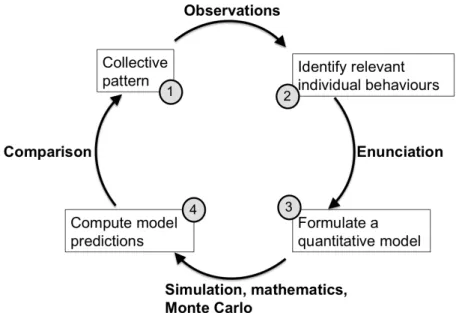
Figure 2.1 – The methodology we use to study collective animal behaviors. It starts (1) with some intriguing collective behavior we want to understand, and continues (based on observation of the system) with a first choice of relevant individual behaviors (2). These behaviors are then precisely translated into a quantitative model (enunciation) from which we predict the emerging collective patterns (3+4). Finally, the predicted pattern is compared to the actually observed pattern (4+1). If this comparison is not satisfactory, we go back to the choice of individual behaviors (maybe an important behavior was missed) or to the model enunciation (have we correctly translated the behavior into quantitative terms? are there statistical biases in the parameter estimation methods?) and redo the cycle until we find a satisfactory prediction of the collective pattern.

The main goal of this methodology is to identify the individual behaviors that can explain some collective behavior we are interested in. It therefore starts with the identification and description of some intriguing collective behavior we want to understand (step 1). In the example cited above this pattern was the construction of a shelter of the right size to protect the queen. The next step is to identify, by direct observation of the biological system, candidate individual behaviors that can explain this collective pattern (step 2). In the case of queen shelter construction this had been done in the early work of P.-P. Grass´e (summarized inGrass´e 1984) and by controlled experimental approaches byBruinsma(1979) in his PhD work. All subsequent modeling work on this shelter construction found their biological inspiration in Bruinsma’s PhD work (Deneubourg, 1977; Courtois and Heymans, 1991; Bonabeau et al., 1998a; Ladley and

Bullock, 2005; Hill and Bullock, 2015). We will illustrate the methodology with the work by

Ladley and Bullock (2005) who selected the following elements from Bruinsma’s work:

• the termites move around randomly on the ongoing construction with a tendency to deposit pellets where previous pellets have been deposited or to move towards such places,

• the pellets themselves are impregnated by the termites with some volatile marking (cement pheromone),

• the queen emits queen pheromone at a constant rate and which diffuses in the air,

• termites only deposit pellets at a certain queen pheromone concentration.

The next step in the methodology is to formulate precisely how these behaviors are translated into a model (step 3), which is in their case a computer simulation model. My physics colleagues

(13)

call this step model enunciation to emphasize that a clear and precise description of this translation of individual behavior into the model is required in this step. By this emphasis there is a clear separation between step 2 (selection of individual behaviors) and step 3 (writing the model), and subsequent critical examination of the work can separately question the decisions made in both steps. Ladley and Bullock (2005) choose to implement construction in a 3D lattice model, where each soil pellet corresponds to a cube. Their pellet carrying termites move around randomly in the empty cells adjacent to the built cubes (according to some precise rules that the authors call logistic constraints) with a bias towards cells with a higher cement pheromone concentration. They have a fixed probability to deposit their pellet. The cement pheromone in the deposited cube decreases/evaporates exponentially. There is a fixed number of pellet carrying termites, and when one deposits its pellet it disappears and a new pellet carrying termite is generated at a random location. The queen is modeled as a fixed template that emits queen pheromone at a constant rate. This pheromone spreads in the empty cells according to a standard diffusion implementation in lattices. Pellets can only be deposited within a fixed range of queen pheromone. This implementation leads indeed to the formation of a dome shaped shelter around the queen (Fig2.2) that compares well with the observed queen shelters inBruinsma (1979) or Grass´e (1984) (step 4).

Figure 2.2 –Termite queen shelter construction according toLadley and Bullock(2005): the pheromone emanating queen is the straight object in the center or the arena, rather evenly spaced pillars are formed at a constant distance around the queen and rise continually, then the space between pillars is filled up to form walls, and the queen is finally covered by a regular dome (Fig fromLadley and Bullock 2005).

Though this model relies on precise quantitative descriptions I would rather call it a qual-itative model because none of the parameters used in the model has been estimated directly from experimental data, nor is the queen shelter described in any quantitatively precise form. Step 4 is therefore limited to a qualitative comparison, and if one is not satisfied with this com-parison it is possible to “play around” with the parameter values (or, in more scientific terms, tune them) until the comparison is satisfying. While this proof of concept is useful to show that the proposed mechanisms are capable to explain the observed collective behavior, Weitz et al.

(2012) has shown in another experimental system that many different mechanisms can produce the same collective outcome, even if the latter is precisely quantified. This illustrates that with a qualitative model we have only limited statistical power to identify/select the underlying in-dividual behaviors. For this reason Camazine et al. (2001) postulates a strict quantitative approach for their methodology:

• the resulting collective structure must be precisely quantified to permit a quantitative (statistical) comparison between observed pattern and model predicted pattern,

• the enunciated individual behavioral rules must be parameterized as good as possible from experimental data on the individual level that are independent of the data/experiments on the collective level.

(14)

With this additional requirement the methodology resembles the well known statistical ‘in-sample out-of-‘in-sample’ model validation concept: the model is fit to part of the data (in-‘in-sample), and model validation is based on how well this fitted model predicts the out-of-sample data. The in-sample data are the one on the individual level on which the parameters of the individ-ual behavioral rules are calibrated, while the out-of-sample data are the one on the collective level. This strict quantitative approach should increase our statistical power to detect and reject “wrong” individual behaviors (in the sense that they are not relevant to the emerging collective pattern) or “wrong” enunciations of these behaviors (in terms of model formulation and parameter estimation). Since the publication of Camazine et al. (2001) this full quantita-tive methodology has been successfully applied in several case studies: cockroach aggregation

(Jeanson et al., 2005; Am´e et al., 2005), cockroach collective decision making (Halloy et al.,

2007;Canonge et al.,2009), corpse-clustering in ants (Theraulaz et al.,2002), collective motion

in fish (Gautrais et al.,2012), ...

2.4 What does it take to understand social insect nest

construc-tion?

Let’s come back to morphogenesis in social insect nest construction as announced in the title. The concepts and examples described in the previous sections make it clear that several mech-anisms are at work: there is self-organization as in pillar construction in termites, there are templates as in termite queen shelter construction, and these templates can even be dynamic either by external changes (day-night, winter-summer) or by internal changes (queen size, the ongoing construction itself). My research goal in the next few years will be to understand the emergence of some termite nest architectures in this framework, with the mathematical and computational tools that are needed for this goal. The rest of this text will retrace my work over the last 14 years to check whether I have the skills to pursue this goal, both conceptually as well as technically. In chapter3I will retrace the work on cockroach aggregation. This work started in 2001, when I came to Toulouse in Guy Theraulaz’s research group, and it was my initiation to the groups theme “collective animal behavior”. Chapter4will review our work on the clustering of objects, in particular corpse-clustering in the harvester ant Messor sanctus. During this work I started to supervise my own students both on the Masters and PhD level. Chapter5will summarize what we know about the mechanisms underlying nest construction in both ants and termites. During this work we also received our first ANR grant that permitted us to create a large data-base of 3D nest-architectures and the presentation of some of these nests in a public virtual museum (http://www.mesomorph.fr). Finally, in chapter 6 I will develop my research program for the next couple of years that involves in particular two PhD students that started their work in fall 2014 or will start it in fall 2015, the jury’s assessment of these perspectives will therefore be highly valuable.

(15)

Chapter 3

Self-clustering of animals (or robots)

The clustering of animals of the same species is a widespread phenomenon in nature (Krause

and Ruxton, 2002). Such clustering can have an adaptive purpose (create a locally favorable

micro climate, better defense against predators, more efficient predation, mate finding,. . . ), but it also includes costs (competition for ressources, more visible to predators, . . . ). Independently of the adaptive nature of this clustering, one can also investigate the behavioral mechanisms that permit the animals to group together. When I arrived in the CRCA in Toulouse in 2001 Rapha¨el Jeanson had just started his PhD and was working on these individual behavioral mechanisms in the case of the aggregation of german cockroach larvae (Blattella germanica, Fig 3.1). These cockroaches frequently aggregate together during the resting phase, Fig 3.1, purportedly to create a favorable microclimate (Dambach and Goehlen,1999). Clustering has also been shown to increase individual growth (Prokopy and Roitberg,2001).

Figure 3.1 –The german cockroach (Blattella germanica): adult male and female (the latter carries an ootheca) and three instars during their development. The bottom row shows the experimental aggrega-tion pattern: 20 cockroach 1st instar larvae are released in a Petri Dish (diameter 11 cm), they first move around to explore the arena, then start aggregating until in the end there is a single or two aggregates.

(16)

3.1 Apply the SO methodology to study cockroach aggregation

behavior

Rapha¨els work required to program cockroach aggregation as an individual based model (IBM) in order to predict the emerging aggregation pattern from his experimentally determined indi-vidual behaviors1. His PhD supervisors Guy Theraulaz and Jean-Louis Deneubourg decided that I could work with him for several reasons: (a) Rapha¨el was new to programming, an inde-pendent implementation by another programmer in a different language would therefore ensure that no major bug distorted his results, (b) my background in model selection could be useful to decide which behaviors are essential to be included in his IBM, and (c) for me this was the ideal opportunity to dive into the world of collective animal behaviors.

Cockroach aggregation behavior has three components: (1) cockroach movement, (2) cock-roach stopping and (3) cockcock-roach departure. Cockcock-roach movement in the experimental arena (Petri Dish with diameter 11 cm) has itself two components, a standard diffusive random walk in 2 dimensions when far (>5 mm) from the Petri Dish wall, and a strong tendency to follow the wall (often calledthigmotactic behavior) for a long time, sometimes making a U-turn (thus a 1-dimensional random walk), before returning to the arena center. This switching between 2-D and 1-D random walk had already been worked out by Rapha¨el and our physics colleagues Richard Fournier and St´ephane Blanco (Jeanson et al., 2003), in particular how to estimate model parameters from the experimental data. Several key ingredients of their model are worth mentioning. The size of the arena permitted to model the 2-D random walk in the arena center with an isotropic phase function (rather than the correlated random walk that describes an animal’s trajectory more precisely,Codling et al. 2008): the longer ballistic phase in the corre-lated random walk had no importance for the emerging cockroach distribution in the arena and parameter estimation for a random walk with isotropic phase function is much simpler than for a correlated random walk, it only required to estimate mean cockroach speed and the mean free transport path from the slope of the net squared displacement (if you are completely lost with this terminology I suggest to readChallet et al.(2005b) for an introduction to correlated random walks and the appendix inCasellas et al.(2008) for the formal link between correlated random walks, isotropic random walks and net squared displacement that actually goes back to

Einstein(1905)). The rate to do a U-turn when following the arena wall was much smaller than

the rate to leave the arena wall, it could therefore be neglected. Sometimes a cockroach stopped and rested for a certain time before moving again. The inclusion of this behavior proved to be essential to correctly predict cockroach density in the arena center as well as along the arena wall. We will come back to the details of this stopping behavior in the next paragraph.

Cockroach stopping behavior was then studied as a function of how many stopped neigh-bors a moving cockroach can detect. This neighbor detection happens by tactile contact with either antenna or cerci, the number of neighbors can therefore be considered as the number of individuals within reach of antenna and cerci (fixed perception radius). Rapha¨el needed in particular to estimate the rate of stopping as a function of the number of stopped neighbors. For spontaneous stops this was rather easy, it was sufficient to measure the time of movement before a spontaneous stop and estimate this rate as the inverse of the mean movement time. Furthermore, the survival curve of the moving times resembled an exponential distribution, the rate can therefore also be estimated as the slope of this survival curve on log-linear scale (technically this means that spontaneous stopping can be modeled as a memory-less or Marko-vian process with a constant stopping rate - the underlying mathematics can be found in any textbook on statistical physics). Estimating the stopping rates when the cockroach senses N

1

A cluster or aggregation can be defined as any assemblage of individuals that results in a higher density than in the surrounding environment (Camazine et al.,2001).

(17)

stopped neighbors required a different technique: Rapha¨el observed all encounters between a moving cockroach and an aggregate of size N and computed the fraction of cockroaches that actually stopped in the aggregate. Assuming a constant speed and a fixed encounter duration between the moving cockroach and an aggregate of size N one can estimate the stopping rate of each N (see Appendix inJeanson et al. 2003). It turned out that the stopping rate increases monotonically with size N - this is a positive feedback, the cockroach has an increased tendency to stop the more stopped neighbors are around it.

Finally, stop duration turned out to be the most tricky part in Raphaël’s model. Fig3.2(a) shows the survival curves of the times an aggregate remained of fixed size N before changing its size (departure or arrival of a cockroach). Contrary to the spontaneous stop survival curve, these curves do not resemble an exponential distribution (that would be a straight line on log-linear scale), at best they resemble the combination of two straight lines. Indeed, when observing the stopped cockroaches more closely, Raphaël saw that some of them remained rather nervous (moving the antenna and cerci), while others appeared to be very calm. The first had on average shorter stop durations than the latter. Raphaël and coworkers therefore suggested that a stopped cockroach can be in two states: a nervous state with a (fixed) high departure rate, and a calm state with a (fixed) low departure rate. The resulting survival curve of such a process would be the superposition of two exponential curves, resulting in such a bilinear pattern. When estimating the associated parameters from his survival curves he found that the fraction of nervous cockroaches decreased with aggregate size N , while the departure rates for both states also decreased with N . In short, the larger the aggregate, the longer the cockroaches tend to stay - this is again a positive feedback.

Figure 3.2 –(a) Survival curves (on log-linear scale) of the stop durations of aggregates of size N = 1, 2, 3 and 4, (b) comparison between the dynamics of the largest aggregate size (with 20 cockroaches in the arena) between experiments, the IBM’s predictions (Social simulations) and the predictions when the two positive feedbacks had been removed from the simulations (Nonsocial simulations). These are Figs 2 and 3 fromJeanson et al. 2003.

The combination of the two positive feedbacks, stop when there are many stopped neighbors and leave when there are few stopped neighbors, results in a strong overall positive feedback that promotes cockroach aggregation. Rapha¨el identified this positive feedback as the core social behavior that promotes cockroach aggregation. Putting all these behaviors together in his simulation code (Fig 3.2(b)) the experimental dynamics of the largest aggregate size were close to the model predictions, but when he removed the positive feedback from this model there was simply no aggregation at all (Nonsocial experiments in Fig 3.2(b)).

(18)

3.2 A first scheme for quantitatively based model selection

Rapha¨el decided to include (or not include) a behavior in his model by comparing the ex-perimental data visually to the model predicted values (for example the fit of the “double exponential” curves in Fig 3.2(a), or the closeness between experimental dynamics and Social simulation dynamics in Fig 3.2(b)). However, while the “double exponential” seemed to fit the survival curves much better than a simple exponential distribution, this criterion does not tell whether the “double exponential” is important with respect to the global aggregation dynam-ics. To test this question one could fit exponential distributions to the survival curves, redo the simulations and compare visually whether the model with “double exponential” distributions improves model predictions. As my modest original contribution to Rapha¨el’s work I tried to develop a quantitative model assessment criterion to decide whether the “double exponential” is indeed necessary (Jost et al.,2002).

We keep the in-sample and out-of-sample framework outlined in section 2.3: estimate all model parameters with data on the individual level (in-sample), then predict the emerging collective level and compare it to the actually observed pattern on the collective level (out-of-sample). On the individual level the stop durations will either be fit to a simple exponential curve or to the double exponential curve, predicting then in both cases the out-of-sample prediction by Monte Carlo simulation. The only difference to Rapha¨el’s will be, following the ideas of model selection theory in Linhard and Zucchini (1986), to define a so-called “discrepancy”, which is simply a quantitative measure of proximity between predicted and observed pattern. Since the predicted pattern is a whole dynamic system (as in Fig3.2(b) I will use the dynamics of the largest aggregate) this discrepancy has to properly weigh the different phases in the dynamics (increasing phase, stationary state). Since Rapha¨el had performed 22 experiments with 20 cockroaches in the arena, we have at each time step 22 largest aggregates from which we compute the cumulative distribution (CDLA, Fig 3.3). Since the cockroaches had to be anesthesized (CO₂) when transferred to the Petri Dish, the beginning of the experiments may have been perturbed due to their waking up. We therefore sampled these dynamics at 20, 40 and 60 minutes only to catch the increasing and the stationary phase.

5 10 15 20 0.2 0.4 0.6 0.8 1 60’ 55’ 50’ 45’ 40’ 35’ 30’ 25’ 20’ 15’ 10’ 5’

Figure 3.3 – The dynamics of the cumulative distribution of the largest aggregate (CDLA), sampled over the 22 original experiments every five minutes. The x-axis is aggregate size (figure taken fromJost et al. 2002).

To get the predicted pattern I computed the cumulative distribution of the size of the largest aggregate for 22 in silico experiments at 20, 40 and 60 minutes, estimating its expected form in a Monte Carlo setup by repeating the 22 experiments 20 times. The discrepancy between these predicted distributions and the observed distributions in Fig 3.3is computed as the sum of weighted squared differences for all aggregate sizes (X2

(19)

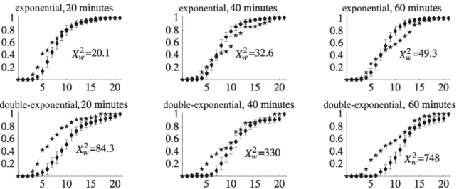
the estimated distributions at each aggregate size (see Fig3.4). The results are ambiguous: the exponential distribution actually produced a smaller overall X2

w, but the CDLA barely moved

between the sampled times, that is it was at stationary state already at 20 min contrary to the observed CDLA. With the double-exponential distribution we recover the dynamics of the CDLA, but overall X2

w is much worse.

Figure 3.4 –Comparison between the observed CDLA at 20, 40 and 60 minutes and the model predicted CDLA, on the top row assuming exponential distributions of the stopping times, on the bottom row assuming double-exponential distributions (figure modified afterJost et al. 2002).

In sum, this first shot at a quantitative model selection approach in the context of collective animal behaviors was not conclusive. We could choose other or more sampled times to give more weight to the dynamics of the CDLA. We could also replace the X_w2 by a Kolmogorov-Smirnov type maximal distance between observed and predicted CDLA. Note also that my discrepancy measure did not account for model complexity (the exponential distributions require one parameter, the double exponential three parameters). The approaching dead-line for the Monte Verit´a workshop put a stop to these first trials, as unsatisfying as they were, but I will come back to this problem of model selection and controlling model complexity in chapter6.

3.3 Cockroach clustering and collective robotics

When I arrived in Toulouse in 2001 our workgroup had also just started as a partner in the European_Leurreproject2 _{under the coordination of Jean-Louis Deneubourg (ULB, Bruxelles,}

Belgium_{). The goal of the Leurre project was to create mixed animal-robot societies and to} apply self-organization theory in order to let the robots control the collective animal behav-ior (Halloy et al., 2007). The robots themselves should merge with the animal group and be accepted by them as one of their own. The principal model organism were cockroaches (Peri-planeta americana, with Colette Rivault from theUniversity of Rennesas the expert partner on cockroach chemical communication, the experiments themselves being done in Bruxelles), the robot partners were Roland Siegwart and Gilles Caprari from the Ecole polytechnique f´ed´erale Lausanne (EPFL), and Toulouse explored how the results achieved with cockroaches could be transferred to a more complex organism, sheep. Gilles had actually already developed an au-tonomous mini-robot, the “sugar cube” robotAlice(Fig3.5_{). For the Leurre project he would}

develop with his partners a new insbot (insect like robot) tailor made for the interaction with 2

(20)

cockroaches. But while waiting for this robot to be engineered (it was actually ready in the 3rd Leurre year) we decided to start collective robotics experiments with the Alice robots in Toulouse (where we already had a couple of these robots, Gilles delivered 20 more to make a nice little robot herd).

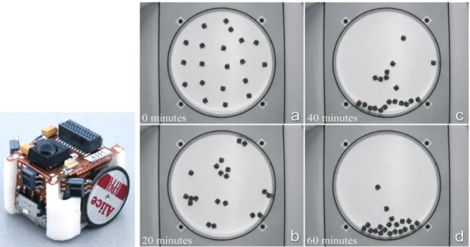
Rapha¨el’s model of German cockroach (Blattella germanica) aggregation served as the start-ing point to implement the same aggregation behavior in the Alice robots. The standard Alice has 4 infrared (IR) sensors to detect objects around them (Fig 3.5), two independent motors to move around freely, they can recognize other Alice by radio contact, and they have about 5h autonomy. A diode on the Alice’s top can also signal its state to an observer. Gilles had developed a library to program Alice in the C-language. I started the work by implementing the single cockroach behavior in a circular arena (Jeanson et al.,2003). We were lucky that at this moment a gifted Master student, Simon Garnier, arrived in the workgroup. He was interested in exactly what we did: study collective animal behavior with the help of experiments, model-ing, simulation and robotics. During his Master internship we implemented together the whole cockroach aggregation behavior (Fig 3.5) and tuned the robots minutely to do quantitatively exactly the same as the cockroaches (Garnier,2004;Jost et al.,2004;Garnier et al.,2008). This was the proof of concept that mini-robot technology could reproduce a simple collective insect behavior at the same scale as the insects.3

Figure 3.5 – An Alice robot with his three infrared sensors pointing forward (there is also one in the back). (a-d) Aggregation process of the Alice in a circular arena (diameter 50cm).

3.3.1 Clustering and collective decision making

Collective decision-making is a cornerstone for the functioning of animal groups: see Sumpter

(2010, Ch 4) for a general review,Camazine et al.(2001, Ch 12) for bee foraging,Beckers et al.

(1990) for ant foraging, Detrain and Deneubourg (2008) for the comparison between bee and ant foraging, Seeley et al. (2012) for bee nest site selection, to cite but a few. For a collective decision to happen there must be a strong positive feedback (Detrain and Deneubourg,2008). Is 3_{In the final mixed societies the insbot had actually a much simpler behavioral program – key to the successful} subtle interaction with cockroaches was to make it smell like a cockroach (Sempo et al.,2006;Halloy et al.,2007).

(21)

the positive feedback in cockroach aggregation (stop where there are many cockroaches, depart when there are few around the cockroach) sufficiently strong to trigger a collective decision? Indeed it is,Am´e et al. (2006) could even show that the process leads to optimal mean benefit for group individuals. Note also that the final experimental setup chosen in the Leurre project to show that the mixed societies worked and that the robots could influence collective behavior was a collective decision setup (Halloy et al.,2007).

After his Master, Simon started a PhD on collective decisions in general under the supervi-sion of Guy Theraulaz. The robot setup developed during his Master (Garnier,2004) continued to serve as a testbed (together with collective foraging in the Argentine ant Linepithema hu-mile). Inside the arena there were two suspended disks of red acrylic glass to provide two shelters from light (very similar to the final setup used in the Leurre project). The robots could move freely under these disks or in the rest of the arena, but they were programmed to stop only under the shelters. The positive feedback implemented previously could therefore only unfold beneath these shelters. Stopped robots light their diode to be detectable below the shelters. See Fig 3.6for the setup and a typical experiment.

In a first setup (Garnier et al.,2005) the robots had the choice between two disks of the same size (14 cm diameter). While a trinomial distribution (distribution of randomly moving animals without a positive feedback between shelter 1, shelter 2, and the rest of the arena) would predict an equal number of robots under each shelter (Fig 3.6B.1), the robot experiments as well as computer simulations show a U-shaped choice distribution, meaning that in each experiment robots cluster preferentially under one of the two disks, but either disk can be chosen with equal probability (Fig3.6B.2-B.3). In a second series of experiments they had a choice between a 10 cm disk and a 14 cm disk: they preferentially chose the 14 cm disk (Fig 3.6A.2-A.3). In a final series of experiments they had a choice between an 18 cm disk and a 14 cm disk: they preferentially choose the 18 cm disk (Fig 3.6C.2-C.3). Garnier et al. (2005) concluded that robots, just as cockroaches, make a collective decision for the larger disk without robots explicitly comparing between the two sites. This could be explained by the higher probability for a randomly moving robot to encounter the larger disk, but robot densities under the larger disk tend to be lower, thus decreasing the strength of the positive feedback. To explore the interplay between these two mechanisms Garnier et al. (2009a) performed further simulation work where they varied the ratio between the two shelter sizes continuously from 0 to 7 (while keeping the arena size always proportional to the sum of the sizes of the two shelters): indeed, the preference for the larger disk had a maximum for a ratio around 2 and then decreased continuously, though still preferring the larger disk but with decreasing asymmetry.

3.3.2 Trail formation in robots: light as a substitute to pheromones

Insect communication relies to a large extent on pheromone communication. Robot technology is still far away from using pheromones in the same way as insects. In Halloy et al.(2007) the insbots were made to smell like cockroaches by glueing filter paper on them that was sprinkled with the pheromone cocktail identified by the group in Rennes (Sa¨ıd et al., 2005). However, the robot had neither control of pheromone emission, nor could it detect the pheromones. This shuts the door to the transfer of many social insect solutions to collective robotics. However, when discussing this problem with Fabien Tˆache (one of the roboticists in Lausanne involved in the Leurre project) we thought that light is very easy to detect by a robot. We thus started fantasizing about a system where light trails are projected by a video-projector, the robot detects the light with two photosensors (to imitate the osmotropotaxic pheromone orientation in ants,

Fraenkel and Gunn 1961), its position being tracked in real time and this information used to

(22)

Figure 3.6 – Collective decisions by the Alice robot: (left) experimental setup with two shelters seen from the top or in a 3D visualization, (right) choice distributions (percentage of cockroaches under the 14 cm diameter disk on the x-axis, number of experiments that ended with this percentage on the y-axis: a dominant bar on the right means the 14 cm disk has been chosen in columns A and C) when the robots had a choice between two disks of sizes 10 cm and 14 cm (column A), between two equal sized disks of 14 cm (column B) and between two disks of sizes 18 cm and 14 cm (column C). The top row shows the expected choice distribution from a trinomial distribution (that has no positive feedback mechanism), the middle row the result of 20 robot experiments with 10 robots each, and the bottom row the result of spatially explicit Monte-Carlo simulations. Figs taken fromGarnier et al.(2005).

(23)

great ideas tend to emerge in parallel in many places. By the time Fabien had developed the first prototype of this system we discovered that the Japanese had had exactly the same idea and were beyond prototypes (Kazama et al.,2004;Sugawara,2005). Nevertheless, Simon took up Fabien’s prototype and adapted it (Fig3.7) to study questions he had faced in the foraging decisions made by argentine ants Linepithema humble (Garnier et al.,2009b). If ants access a food source via a bridge with two equal length branches they make a collective decision and most traffic will circulate on only one of these branches (Beckers et al.,1992b;Dussutour et al.,

2004). The underlying mechanism is the ant’s choice function when facing a Y junction with pheromone concentrations on the left and on the right: this choice function is highly non-linear, with small differences in pheromone concentrations amplifying the turning bias towards the higher pheromone side.4 _{Simon constructed the same setup for the Alice robot (Fig} _3.7_(b)):

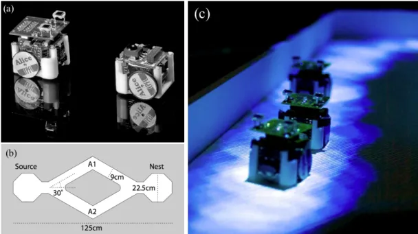
Figure 3.7 – The Alice light trail experiments: (a) An Alice equipped with two photosensors that can detect independently light intensity (similar to the two ant antennas that detect pheromone concentra-tion), (b) the simple experimental setup used, with a diamond shaped channel system between the “nest” and the “food”, (c) three Alice robots following the projected light trail. Figs modified after Garnier et al.(2007).

as soon as the robot leaves the nest or the source it switches on its LED, is detected by the tracking system which projects on this position a light spot (pheromone) which decays slowly with an exponential type decay. The robots perform a standard correlated random walk unless they detect light, in which case they turn preferentially towards the higher light intensity (Fig

3.7(c)). With this “simple” setup the robot herd produced the same branch selection as the ants (Garnier et al.,2007).

The next step was to let the robots navigate in a more complex network with variable geometry. Fig 3.8 shows the used setups: they had 3 loops and the junctions were either symmetrical or asymmetrical. Argentine ants tend to choose the branch where they have to turn less, and they found the shortest path faster in the asymmetrical setup than in the symmetrical

4

Note that ants do not compare the pheromone concentrations between the left and right branch, they simply detect the pheromone concentrations with their two antenna and the net difference influences the magnitude of turning behavior according to a Weber’s law. Perna et al.(2012) showed this experimentally and further showed analytically that this simple behavior combined with some directional noise can result in the Deneubourg type non-linear choice function (Beckers et al.,1992b) usually used in the literature.

(24)

one (Garnier et al.,2009b). Note that such asymmetries in trail bifurcations had been found in real ant trails (Jackson et al.,2004). Simulations inGarnier et al.(2009b) had shown that the ant’s preference for small deviations could explain this difference and that foraging efficiency (measured in the simulations as the number of ants going from S to T or from T to S) was three times higher in the asymmetrical setup. The implementation in the robotics system (Garnier

et al.,2013) showed two things: (a) the light “pheromone” recruitment system combined with

asymmetrical junctions resulted in the highest recruitment efficiency (Fig3.8), (b) the robots did not need to know the turning angle to the next branch in order to bias their choice to the lesser angle, the “inertia” of their correlated random walk combined with obstacle avoidance behavior and the amplification power of pheromone trails was sufficient to reproduce this behavior.

Figure 3.8 –(left) The 3 loop networks used inGarnier et al.(2013) with either symmetrical junctions (wherever the robot comes from, it has to turn the same angle) or asymmetrical junctions (the angle to turn depends where the robot comes from and where it goes). S marks the starting area, T the target area. (right) Foraging efficiency (measured by the number of successful trips) of the robots in the symmetrical (S) or asymmetrical (A) setup and with (+P) or without (-P) light “pheromones”. Figs taken fromGarnier et al.(2013).

When we had started working with robots (Garnier, 2004) we had only in mind to use social insect behavior as a bio-inspiration for collective robotics, with the additional challenge to reproduce cockroach behavior on the right scale. However, when Jean-Louis Deneubourg remarked provocatively that this work had taught us nothing about biology we were nevertheless somewhat disappointed. Continuing to think about this problem we meanwhile nevertheless think that collective robotics experiments can also help us answer biological questions. Garnier

(2011) mentions several reasons:

1. robots require a complete specification and implementation of the individual behavior in a given environment (similar to simple computer simulations),

2. robots are physical entities that move around in physical space with all its constraints (this is more difficult to include realistically in computer simulations). It was exactly this property that made robots the tool of choice in the mixed societies study (Halloy et al.,

2007), and robots, as modern lures, are used in many other areas of behavioral research,

(25)

that taught us that robots do not need to measure angles in order to favor low direc-tional changes in a Y-maze – so why should ants need to know such angles to show their behavioral bias towards low angle directional changes?),

4. robots are simply very “cool” gadgets that help direct attention to our questions and that are of great use with students to illustrate biological ideas (more so than simulations which are less transparent for many biology students). The last point is well illustrated by the media coverage given to Garnier et al.(2013).

In sum, collective robotics will remain in the behavioral biologist’s toolbox, in particular because robot behavior is completely controlled by the programmer and their physical presence make interactions with real animals possible.

(26)

Chapter 4

Object-clustering: corpse clustering

in ants

The first step towards nest construction is the clustering of objects. It was the clustering of soil pellets by termites that inspiredGrass´e(1959,1967) to create his stigmergy concept (Theraulaz

and Bonabeau,1999). One of the first experimental demonstrations of self-organization in social

insect nest construction was with Leptothorax ants that chose small cavities for nesting where they build additional walls by simply bulldozing sand pellets together (Franks et al.,1992). In the last centuryChr´etien(1996) invented another clustering paradigm to study the underlying mechanisms: the aggregation of dead nest mates by the black garden ant Lasius niger. When an ant dies within its colony the corpse is usually picked up by some nest mate and transported outside the nest (Wilson et al.,1958;Haskins and Haskins,1974;Howard and Tschinkel,1976) where it is aggregated in refuse piles (or middens) together with other waste from the nest (Fig

4.1).

Figure 4.1 – Messor sanctus is a harvester ant living around the Mediterranean. They harvest grains

from plants and store them in their underground chambers as food reserve. Waste, such as the corpses of dead conspecifics, is expelled from the nest and accumulated by the ants in refuse piles or middens, purportedly for nest hygienics. They have often erroneously been called “cemeteries”, but corpses are treated just as any other garbage object.

(27)

waste, let pathogens grow on them: expelling them from the nest reduces the risk of infection and aggregating them reduces the risk for foraging ants to get in contact with contaminated material. Workers identify corpses by their production of fatty acids (eg. oleic acid, Wilson

et al. 1958;Howard and Tschinkel 1976) and they usually never bring the corpses back into the

nest (but see alsoGordon 1983who found that this behavior may depend on the social context). This last property was used byChr´etien(1996): she distributed ant corpses in a flat arena and let the ants arrive spontaneously in the arena. The ants quickly started assembling/aggregating the corpses into piles, and since the corpses are never brought back to the nest the dynamics of the complete clustering process and the fate of all corpses could be observed by simply filming the experimental setup. Chr´etien (1996) found that any corpse found by the ant had the same probability to be picked up (she did not assess whether local corpse density changes this probability, she only varied their distance from the nest), that they are then transported a certain distance away from the nest entrance and preferentially deposited at the arena border or on other objects such as corpse piles (spontaneous depositing occurred, but with a low rate). A simple simulation model (1-dimensional cellular automaton with a cell line along the arena border, ants moving from cell to cell at constant velocity, with a constant probability to pick up an encountered corpse, while varying the deposition probability with local corpse density) permitted her to reproduce the observed aggregation patterns qualitatively.

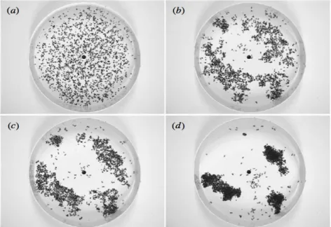
To fully apply the methodology outlined in section 2.3 Theraulaz et al. (2002) started the same kind of experiments with the harvester ant Messor sanctus1 (Fig 4.2). Since Chr´etien

(1996) had observed that corpses are mostly deposited along the arena border and, once there, remained there even if picked up again, they chose to distributed the corpses in the beginning homogeneously along the arena border. As can be seen in Fig 4.2 the aggregation dynamics took indeed place along the arena border.

Figure 4.2 –(left) Corpse-clustering in Messor sanctus in a circular arena when the corpses are initially distributed homogeneously along the arena border. The nest is beneath the arena and exploring ants enter the arena along a wood stick through the hole in the centre of the arena. Corpses are distributed in the beginning regularly along the arena border and apparently remain there during the hole aggregation process. (right) Corpse depositing (top left) and picking up (bottom left) probability as a function of pile size, with the calibrated theoretical curve; survival curve of transport distance (right) that resembles an exponential distribution. (Figs 1 and 3 fromTheraulaz et al. 2002).

In a first series of experiments they measured the probability for a corpse transporting ant 1_{Note that this species is also called Messor sancta, but since the latin root ofMessor is masculine L. Passera} argues that the adjective should also be masculine – I go along with L. Passera in this text.

(28)

to deposit a corpse on a pile of size 1, 5, 10, 20, 30 or 50 corpses, for a free exploring ant to pick up a corpse on the same pile sizes, and the transport distance before depositing a corpse (Fig 4.2(right)). We can see a similar positive feedback as in cockroach aggregation: pick up corpses at low densities and deposit them preferentially at high corpse densities. The increasing scarcity of isolated corpses and the low picking up rates of corpses in piles act a as a negative feedback that maintain the dynamical system finally in a stationary state.

How to model these observed behaviors? Since transport distance was distributed like an exponential distribution (memory less process) spontaneous corpse deposition can be modeled with a constant deposition rate kd (estimated as the slope of the survival curve on log-linear

scale). Depositing and picking up behavior are more complicated. Let Φ_c be perceived corpse density (up to 1 cm behind and in front of an ant), ρ a fixed free (non-transporting) ant density, a the density of transporting ants and c the corpse density. The picking-up rate can then be modeled as α3ρ

α4+Φc, and the deposition rate as

α1Φc

α2+Φc. Inversion techniques permitted to estimate the parameters α_i from the observed probabilities: the fitted functions are shown in Fig 4.2

(the full details of the inversion process can be found inWeitz 2012). Given the uncertainties in the measured probabilities the fitted functions well describe individual depositing and picking up behavior. Finally, they also measured average ant speed v and the mean distance following the border before making a U-turn, mean free transport path l.

Given all this information an individual based model (IBM) could me implemented on a computer in order to predict the emerging clustering dynamics and compare them to the observed dynamics. But one can also derive from these parameterized individual behaviors a mean filed model in the form of partial differential equations (PDE):

∂c ∂t = Ω(c, a) ∂a ∂t = −Ω(c, a) + D ∂2a ∂x2 | {z } I Ω(c, a) = v      kda |{z} II + α1Φc α2+ Φc a | {z } III + α3ρ α4+ Φc c | {z } IV     

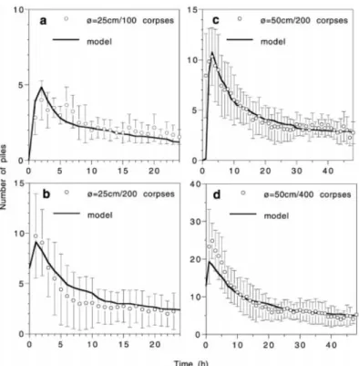
Part I represents the diffusive random walk of transporting ants along the arena border (follow the border and make a U-turn at rate 1/l) with the diffusion coefficient D = vl/2. Note that ants usually deposited their corpse before making a U-turn, diffusion could therefore be neglected. Part II is the increase in corpse density through a spontaneous deposition (without any corpses within the ants perception area), part III the increase due to corpse induced deposition, and part IV corpse picking up. Numerical simulations of this set of equations showed that the model perfectly predicts the observed clustering dynamics, illustrated in Fig 4.3 for the case of the dynamics of the number of clusters.

Furthermore, the analysis of the equations showed that no aggregation should occur below a certain corpse density (this density is therefore a bifurcation parameter). This prediction was also experimentally verified. Overall, Theraulaz et al. (2002) is an example of the completely applied methodology (section 2.3) in order to identify the underlying behavioral mechanisms.

To show the importance of doing the whole methodology, in particular to predict the emerg-ing pattern from experimentally observed and quantified individual behaviors, physics PhD student S´ebastian Weitz (see also his other work below) choose in the methodological paper

Weitz et al. (2012) 6 different behavioral models and fitted them only to the collective data in

(29)

parame-Figure 4.3 – Dynamics of the number of piles: comparison between model predictions (solid curves) and experimentally observed values (mean±sd) for arena _{=25 cm with 100 and 200 corpses, and for} arena_{=50 cm with 200 and 400 corpses (Fig 5 from}Theraulaz et al. 2002).

ters. The six models were various combinations of three behavioral traits: (a) inter individual variability: picking-up and deposition statistics depend on an activity level that is constant in time but varies from ant to ant, (b) temporal correlation (or memory effects): the propensity to pick-up or deposit a corpse decreases as the time since the last behavioral action (deposit or picking-up) has elapsed,(c) picking-up inhibition: the picking-up rate of an object decreases with increasing local corpse density. Note that deposition rate increased in all six models with perceived corpse density. Table 4.1lists which behavioral traits were included in the six tested models.

Table 4.1 – The six different models calibrated by Weitz et al. (2012) to the emergent pile number statistics inTheraulaz et al.(2002).

behavior: inter-individual variability temporal correlation picking-up inhibition

model 1 no no no

model 2 no no yes

model 3 yes no no model 4 yes no yes model 5 no yes no model 6 no yes yes

Weitz et al.(2012) first showed that all six models could be calibrated to fit perfectly well the

collective pattern in Fig4.3. He then showed analytically that even if the precision of the data on the collective level were arbitrarily good one could not select a best fitting model: hence the need to study the underlying individual behaviors directly in dedicated experiments. Redoing