HAL Id: tel-01077977
https://tel.archives-ouvertes.fr/tel-01077977
Submitted on 27 Oct 2014HAL is a multi-disciplinary open access archive for the deposit and dissemination of sci-entific research documents, whether they are pub-lished or not. The documents may come from teaching and research institutions in France or
L’archive ouverte pluridisciplinaire HAL, est destinée au dépôt et à la diffusion de documents scientifiques de niveau recherche, publiés ou non, émanant des établissements d’enseignement et de recherche français ou étrangers, des laboratoires
Planning optimization in prostate and head-and-neck
radiation therapy
Pengcheng Zhang
To cite this version:
Pengcheng Zhang. Planning optimization in prostate and head-and-neck radiation therapy. Signal and Image processing. Université Rennes 1, 2014. Chinese. �NNT : 2014REN1S042�. �tel-01077977�
ANNÉE 2014
THÈSE / UNIVERSITÉ DE RENNES 1
sous le sceau de l’Université Européenne de BretagneEn Cotutelle Internationale avec Southeast University, Nankin, Chine
pour le grade de
DOCTEUR DE L’UNIVERSITÉ DE RENNES 1
Mention :Traitement du Signal et TélécommunicationsEcole doctorale Matisse
présentée par
Pengcheng ZHANG
Préparée à l’unité de recherche LTSI – INSERM U1099
Laboratoire Traitement du Signal et de l’Image
Université de Rennes 1, France
Laboratory of Image Science & Technology (LIST)
Southeast University, Nanjing, Chine
Optimisation de
la planification
en radiothérapie
prostatique et
ORL
Soutenance à Nankin, Chine le 02/07/2014
devant le jury composé de :
Pascal FRANCOIS
Physicien Médical, CHU de Poitiers / rapporteur Zhiguo GUI
Professeur, North University of China / rapporteur Baosheng LI
PUPH, Shandong Cancer Hospital and Institute / examinateur Limin LUO
Professeur, Southeast University / examinateur Huazhong SHU
Professeur, Southeast University / directeur de thèse Renaud DE CREVOISIER PUPH, Université de Rennes 1 / directeur de thèse
Optimisation de la planification en radiothérapie
prostatique et ORL
Le cancer correspond à une prolifération cellulaire anormalement importante, la tumeur, au sein d’un tissu sain dont la survie est alors menacée. Selon les dernières estimations du Centre international de recherche sur le cancer (CIRC) et de l'Organisation mondiale de la Santé (OMS), environ dix millions de nouveaux cas de cancer sont diagnostiqués chaque année, avec un peu plus de la moitié des cas dans les pays en développement. En 2015, ce nombre devrait atteindre environ 15 millions de cas, dont les deux tiers dans les pays en développement. Le traitement du cancer en Chine est ainsi une tâche difficile, le taux de mortalité par cancer ayant augmenté de près de 30% au cours des 20 dernières années. En 2008, les nouveaux cas de cancer ont atteint 2,82 millions et les prévisions donnent un nombre de 21 millions en 2030.
La radiothérapie est devenue l’un des trois principaux traitements du cancer, avec la chimiothérapie et la chirurgie. Elle repose sur l’utilisation de radiations, généralement des photons, pour détruire les cellules cancéreuses en bloquant leur capacité à se multiplier. L’objectif de la radiothérapie est de délivrer une dose prescrite à la tumeur tout en minimisant l’irradiation des tissus sains environnants. Un traitement par radiothérapie repose sur deux étapes principales : (i) la planification du traitement, durant laquelle les caractéristiques de l’irradiation sont optimisées suivant l’anatomie du patient telle qu’elle est représentée par une image scanner ; (ii) la délivrance du traitement fractionnée en une série de séances (par exemple 40 fractions pour un traitement du cancer de la prostate). Si les nombreuses avancées technologiques des dernières années, que ce soit en imagerie (scanner, IRM et TEP), pour le calcul de dose (superposition 3D, Monte-Carlo) ou pour la délivrance du traitement (IMRT, SRS, IGRT), ont permis d’améliorer considérablement la précision du traitement, un certain nombre de problématiques restent ouvertes. Ainsi, lors de la planification, les algorithmes de calcul de dose peuvent encore souffrir d’imprécisions. La prise en compte de paramètres radio-biologiques lors de cette planification reste aussi à améliorer. De même, l’impact des incertitudes géométriques lors de la délivrance du traitement doit être compensé. Enfin, dans une stratégie de radiothérapie adaptive, permettant de prendre en compte des modifications anatomiques en cours de traitement par des replanifications, les scénarii optimaux restent à identifier. Ce travail de thèse s’attache à proposer des solutions à ces différents enjeux.
Lors de la planification, la balistique de traitement est optimisée suivant l’anatomie du patient telle qu’elle est représentée par le scanner de planification. Cette étape repose notamment sur la simulation, pour une balistique de traitement donnée, de la matrice de dose reçue par les différents organes. Différentes méthodes sont utilisées pour cette simulation dans un objectif de compromis entre précision et rapidité de calcul. L’approche la plus fréquemment utilisée est celle du Pencil Beam, reposant sur la convolution/superposition de faisceaux élémentaires. Cette approche a cependant certaines limites : (i) l’inclinaison des faisceaux élémentaires est négligée ; (ii) la correction des hétérogénéités de tissus est approximative ; (iii) ces approches restent couteuses en temps de calcul. Dans ce travail, l’approche classique du Pencil Beam a été modifiée en considérant un système de coordonnées sphériques adapté à la géométrie des faisceaux, en modifiant le mode de correction des hétérogénéités et en accélérant le calcul grâce au calcul des convolutions par la transformée de Fourier rapide. L’approche proposée a été comparée à la méthode AAA en considérant le calcul de Monte-Carlo comme référence. Différents fantômes numériques (eau, eau et insert de poumon, eau et insert d’os, eau et inserts de poumon et d’os) ont été utilisés. La méthode proposée a ainsi montré une meilleure précision que la méthode AAA, avec cependant des erreurs importantes aux niveaux des interfaces. Par ailleurs, le calcul par transformée de Fourier permet d’accélérer le calcul d’un facteur 40, au prix toutefois d’une dégradation de la précision des résultats. Il serait ainsi intéressant, dans de futurs travaux, de combiner les deux approches : le calcul par transformée de Fourier lorsqu’une estimation grossière de la dose est suffisante, puis par la méthode par superposition pour affiner le résultat de l’optimisation.
Toujours lors de la planification, une fois que la matrice de dose a été simulée, une fonction de coût est considérée de façon à pouvoir comparer quantitativement différentes balistiques. Cette fonction de coût repose généralement sur des contraintes dosimétriques simples issues notamment de l’histogramme dose-volume, et ne prend pas en compte la complexité de la réponse biologique de la tumeur ou des tissus sains. Ceci pourrait être corrigé par l’incorporation de modèles radio-biologiques tels que les modèles NTCP (probabilité de toxicité des tissus sains). Cependant, l’incorporation de tels modèles est compliquée par leur non-linéarité et non-convexité, rendant ainsi l’optimisation du plan de traitement beaucoup plus complexe. Dans ce travail, un critère radio-biologique correspondant à l’équivalent convexe du modèle NTCP a été utilisé. Une fonction de coût incorporant à la fois ce critère radio-biologique (pour limiter l’irradiation des tissus sains) et des critères physiques (pour assurer la couverture de la cible) a alors été proposée pour constituer un modèle hybride physique-biologique. Cette fonction de coût, grâce à l’expression de ses dérivées premières, a été couplée à une optimisation de la fluence par la méthode BFGS. L’évaluation de cette approche a été réalisée sur les données de dix patients traités pour un cancer de la prostate. Une comparaison à la méthode classique reposant uniquement sur des critères dose-volume a été menée. Elle a montré que la méthode
méthodes d’optimisation (recuit simulé et optimisation non-linéaire). Cette étude a montré que notre approche fournit de meilleurs résultats en un temps de calcul inférieur. Les perspectives de ce travail consistent notamment en l’extension de l’approche proposée pour optimiser directement les paramètres machine de façon à fournir un plan de traitement réalisable par l’accélérateur.
Lors de la délivrance du traitement, des modifications anatomiques et des erreurs de positionnement du patient peuvent survenir. Elles constituent des incertitudes géométriques qui peuvent être divisées en erreurs aléatoires et erreurs systématiques. Pour compenser les erreurs aléatoires lors de la planification, différentes approches ont été proposées, comme la méthode de simulation stochastique ou la méthode de convolution de la dose. Ces méthodes entraînent cependant une expansion du volume cible clinique (CTV,
Clinical Target Volume). Pour éviter cette expansion, l’approche du « robust beam profile » a
été proposée, reposant essentiellement sur une augmentation de la fluence au bord des faisceaux. Différentes méthodes de déconvolution ont été utilisées pour obtenir le nouveau profil de faisceau, avec cependant des limites, notamment la présence de hautes fréquences autour des bords du faisceau. Dans ce travail, une approche de déconvolution combinant une décomposition en séries de Taylor et un filtrage avec un filtre de Butterworth a été proposée pour compenser les erreurs aléatoires. Elle a été comparée avec deux autres méthodes de déconvolution sur deux cartes de fluence 2D et un cas prostatique. Les résultats ont montré l’efficacité de la méthode proposée, qui permet de réduire les oscillations de haute fréquence ainsi que la présence de points chauds et froids des profils de fluence.
Toujours lors de la délivrance du traitement, en cas de variation anatomique importante, telle une fonte tumorale en radiothérapie ORL, une ou plusieurs replanifications du traitement peuvent s’avérer nécessaires, notamment pour limiter l’irradiation des glandes parotides. En s’appuyant sur des données recueillies lors d’un protocole clinique en ORL (projet ARTIX) impliquant une replanification hebdomadaire, 31 scénarii différents de replanification, suivant le nombre et les moments des replanifications, ont été simulés. Ainsi, pour chaque scenario, les doses reçues par les patients ont été calculées pour chaque semaine suivant la planification considérée dans le scenario (planification initiale ou replanification). Les critères de comparaison ont été extraits de la dose cumulée reçue au cours de l’ensemble du traitement, calculée grâce au recalage élastique entre délinéations des organes à la planification et lors du traitement. Les critères de couverture de la cible tumorale étant systématiquement respectés, l’analyse s’est focalisée sur la dose reçue par les parotides. Les résultats obtenus sur onze patients ont permis d’identifier les scénarii optimaux de replanifications avec notamment un scénario, optimal pour les deux parotides, à trois replanifications réalisées aux semaines 1, 2 et 5. Ce scénario de replanification permet de diminuer significativement la dose reçue par les parotides puisque le risque de toxicité, établi par le modèle NTCP, est réduit de près de 9%. La suite de ce travail porte sur
façon à proposer des critères de déclenchement d’une replanification dans un contexte de radiothérapie adaptative.
En conclusion, nous présentons dans ces travaux différentes méthodes pour l’optimisation des plans de traitement en radiothérapie des cancers de la prostate et ORL. Ces méthodes ont été évaluées et, chacune à son niveau, permettent d’améliorer les plans de traitement. Les perspectives de ce travail concernent la combinaison de ces méthodes dans un processus complet de planification pour évaluer leur impact dans un contexte clinique.
Publications :
Journaux :
[1] Pengcheng Zhang, Jian Zhu, Yuanjin Li, Huazhong Shu. Improved algorithm of multileaf collimator field segmentation. Journal of southeast university (Natural Science Edition), 2012, 42(5):875-879. (en Chinois)
[2] Pengcheng Zhang, Renaud De Crevoisier, Antoine Simon, Pascal Haigron, Jean-Louis Coatrieux, Baosheng Li and Huazhong Shu. A new deconvolution approach to robust fluence for intensity modulation under geometrical uncertainty. Phys Med Biol, 2013, 58(17):6095-6110.
[3] Pengcheng Zhang,Antoine Simon, Renaud De Crevoisier, Pascal Haigron, Mohamed Hatem Nassef, Baosheng Li and Huazhong Shu. A new pencil beam model for photon dose calculations in heterogeneous media, Physica Medica, accepted.
[4] Pengcheng Zhang, Antoine Simon, Huazhong Shu, Pascal Haigron,Caroline Lafond, Jean-Louis Coatrieux, Jian Zhu, Baosheng Li and Renaud De Crevoisier. IMRT optimization including the equivalent convex NTCP constraint, submitted.
Conférence :
[5] Pengcheng Zhang, Huazhong Shu, Antoine Simon, Pascal Haigron and Renaud De Crevoisier. A new pencil beam model for photon dose calculations. The 2013 6th International Conference on BioMedical Engineering and Informatics (BMEI 2013)
Planning Optimization in Radiation Therapy
of Prostate and Head-and-Neck
Chapter I. Introduction ... 6
I.1. Radiotherapy in cancer treatment ... 6
I.2. Considered challenges in radiation therapy plan optimization... 7
Chapter II. A new pencil beam model for photon dose calculations ... 10
II.1. Introduction ... 10
II.2. Kernel computation in a modified spherical coordinate system ... 11
II.2.1. Modified spherical coordinate system ... 11
II.2.2. Getting the pencil beam kernels ... 12
II.2.3. Extracting the parameters of pencil beam kernels ... 12
II.3. Dose calculations with superposition method ... 13
II.3.1. Dose calculations in water phantom ... 13
II.3.2. Dose calculations in heterogeneous media ... 13
II.4. Dose calculation acceleration using FFTC ... 16
II.5. Validations of dose calculation methods: comparison with AAA and MC methods ... 16
II.6. Results ... 17
II.6.1. Water phantom ... 17
II.6.2. Lung slab phantom ... 18
II.6.3. Bone slab phantom ... 19
II.6.4. Lung and bone block phantoms ... 20
II.6.5. Computation time... 21
II.7. Discussion ... 21
II.8. Conclusion ... 22
Chapter III. IMRT optimization incorporating equivalent convex NTCP constraint ... 23
III.1. Introduction ... 23
III.2. Advantages of biological cost functions ... 24
III.2.1. Limitations of dose-volume-based treatment planning ... 24
III.2.2. Advantages of biological cost functions over dose-volume cost functions . 25 III.3. Methods and Materials ... 25
III.3.1. Dose calculations ... 25
III.3.2. Equivalent convex NTCP constraint ... 25
III.3.3. Hybrid physical-biological model ... 26
III.3.4. Optimization method of the fluence elements ... 27
III.3.5. NTCP-based optimizations proposed by Mohan et al and Stavrev et al ... 28
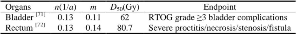
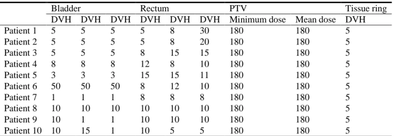
III.3.6. Organ delineation and dose prescription for 10 patients ... 29
III.3.7. Software for optimization and comparison test ... 29
III.4. Results ... 30
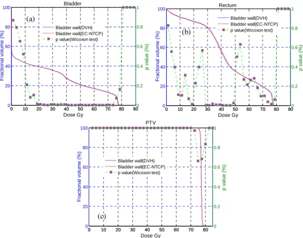
III.4.1. Comparison of the proposed method with dose-volume-based optimization ... 30
III.4.2. Comparison of the proposed method with SA and NP ... 33
III.5. Discussion ... 34
III.6. Conclusion ... 36
IV.1. Introduction ... 38
IV.2. Methods and Materials ... 39
IV.2.1. The beam profile deconvolution with the series expansion method ... 39
IV.2.2. 1D beam profile deconvolution ... 39
IV.2.3. Extension to 2D fluence deconvolution ... 42
IV.3. Results ... 43
IV.3.1. Results for a regular 2D fluence map ... 43
IV.3.2. Results for an IMRT field ... 46
IV.3.3. Results for a prostate case ... 48
IV.4. Discussion and conclusion ... 51
Chapter V. Assessment of the optimal time and number of replannings in head-and-neck cancer adaptive radiotherapy to spare the parotid glands ... 53
V.1. Introduction ... 53
V.2. Purpose and general framework of the study ... 53
V.3. Materials ... 55
V.3.1. Patients and tumors ... 55
V.3.2. Treatment and planning... 55
V.3.3. Weekly dose estimations in cases of replanning ... 56
V.4. Methods for dose accumulation ... 56
V.4.1. Registration algorithm... 56
V.4.2. Aligning the dose distributions ... 57
V.4.3. Calculating the accumulated dose ... 58
V.4.4. Analyzing the cumulated dose and estimating the optimal scenario ... 58
V.5. Results ... 59
V.5.1. Anatomical variations occurring during the 7 weeks of treatment ... 59
V.5.2. Accumulated parotid gland dose distributions without replanning (compared to the planning) ... 60
V.5.3. Accumulated parotid gland dose distributions corresponding to 31 scenarios of replannings ... 61
V.5.4. Optimal number and time of replannings ... 64
V.5. Discussion ... 65
V.6. Conclusion ... 66
Chapter VI. Conclusions ... 67
Abbreviations
AAA Anisotropic analytical algorithm
ART Adaptive radiotherapy
CT Computed tomography
CTV Clinical target volume
DV Dose-volume
DVH Dose volume histogram
EUD Equivalent uniform dose
FFTC H&N ICRU
Fast Fourier transform convolution Head-and-Neck
International Commission on Radiation Units and Measurements
IMRT Intensity-modulated radiation therapy
L-BFGS limited-memory Broyden-Fletcher-Goldfarb-Shanno algorithm
MC Monte Carlo
NTCP PG
Normal tissue complication probability Parotid gland
PTV RT SRS
Planning target volume Radiation therapy
Stereotactic radiosurgery TCP
TPS
Tumor control probability Treatment planning system
Chapter I. Introduction
In this introduction, we briefly present the crucial role of radiotherapy in the treatment of cancer. We introduced afterwards the addressed issues in the different aspects of radiation therapy that we considered in this work: pencil beam dose calculations, intensity modulated radiation therapy (IMRT) optimizations, geometric uncertainties in IMRT, and adaptive radiotherapy (ART) of head-and-neck cancers.
I.1. Radiotherapy in cancer treatment
Cancer has become a common disease which seriously threats the human health. According to recent estimates of the International Agency for Research on Cancer (IARC) and World Health Organization (WHO), approximately ten million new cancer cases are being detected per year world-wide, with slightly more than half of the cases occurring in
developing countries [1]. By the year 2015 this number is expected to increase to about 15
million cases, among which two thirds will occur in developing countries. The cancer prevention in China is a challenging task. The cancer mortality rate has increased by
nearly 30% in the past 20 years [2]. In 2008, new cancer cases reached 2.82 million, and
this number will increase to 21 million in 2030.
Radiation therapy is one of the three major means for tumor treatment, together with surgery and chemotherapy. According to recent estimates of the WHO, the tumor cure rate is about 55% (with a high variability depending on the tumor), whereas the
contribution of radiation therapy is up to 40% to cure the patients [2]. Compared to
surgery, radiation therapy conserves the integrity of the organ affected by the tumor and aims also to keep the organ functionality to limit the side effects and maintain a high quality of life after the treatment.
The radiations used for cancer treatment are ionizing radiation, which can be grouped into two major types: photons (X-rays and gamma rays), which are most widely used in cancer treatment, and particle radiation (such as electrons, protons, neutrons, carbon ions, alpha particles, and beta particles). In this thesis, we mainly focus on the radiotherapy of external photon beams. Ionizing radiation damages the DNA (DNA double strand breaks ) of the cells within both normal tissues and tumors, and makes
them unable to divide and grow [3]. Although radiation is directed at the tumor, the
surrounding normal tissues are also inevitably affected by the radiation and therefore damaged. However, the normal tissues and tumors are prone to different biological reactions to the radiation. Radiation therapy is based on the differential effect of ionizing radiations, killing the tumor cells and preserving in a certain extent the healthy tissue due to the ability of the normal cells to repair the DNA double stand breaks. The goal of radiation therapy is therefore to maximize the dose delivered to tumors while minimizing exposure to healthy tissues, i.e. improving tumor control probability (TCP) while reducing the normal tissue complication probability (NTCP).
A radiotherapy treatment can be divided in two main steps: (i) the treatment planning during which the treatment parameters are defined and optimized according to the prescription and the patient’s anatomy; (ii) the treatment delivery, fractionated in a series of daily fractions.
Advances in imaging technologies (CT, MRI and PET), dose calculation algorithms (3D superposition, Monte Carlo) and dose delivery techniques (IMRT, SRS, IGRT) have made it possible to deliver the prescribed dose in a high conformal fashion to the treatment volume, while sparing relatively well surrounding normal tissue. Radiation therapy has therefore gradually been developed towards a “precise identification and
characterization of the tumor, precise planning, and precise treatment” [4]. The treatment
plan optimization is performed by the treatment planning system (TPS) which needs a lot of key technologies, such as rapid 3D reconstructions, high-precision 3D dose calculations, plan optimizations and inverse planning.
This thesis focused on different challenges concerning plan optimization methods.
I.2. Considered challenges in radiation therapy plan optimization
Many methods have been proposed to improve the quality of IMRT plans considering different aspects, such as dose calculations, plan optimizations, geometric uncertainty corrections and ART techniques. However, several challenges are remaining, including the following ones (cf. Fig. 1.1).
Figure 1.1 Global workflow of RT treatment and position of the different parts of the work.
Dose calculation algorithms play a crucial role in modern TPS. It creates the link between the chosen treatment parameters, and the observed clinical outcome for a specified treatment technique. The ICRU recommends that the dose to the radiation
therapy target volume should be delivered with an accuracy of 5% or better [5]. An
improvement of 1% in dose accuracy may result in an increase of 2% in cure rate for
early stage tumors [6]. Hence, some sophisticated methods have been developed to
improve the accuracy of dose calculations, such as kernel based methods and Monte Carlo (MC) methods. However, the higher is the accuracy of the algorithm, the more computation time is needed for dose calculations. In inverse planning optimization, dose
calculations might be repeated many times (usually from 10’s to 1000’s) [7]. The pencil
beam approach is frequently used in dose calculations to achieve a good compromise between speed and accuracy, which is one of the crucial challenges for the development of modern dose calculation algorithms. However, this pencil beam approach suffers from limitations. Firstly, if the rays from the source are divergent, most pencil beam models, consider parallel beamlets, resulting to imprecision. Secondly, the correction of heterogeneities involves approximations, especially considering the depth-directed components. In this part of the work, we proposed to improve the pencil beam algorithm, without increasing the computation time, by considering a modified spherical coordinate system and by modifying the heterogeneities correction method. Moreover, in order to accelerate the computation, we considered the use of the Fast Fourier Transform to perform the convolutions.
Still in the planning step, the most commonly used approach in IMRT planning is the optimization approach, in which the best physically and technically possible treatment plan is iteratively searched. Optimization is mathematically defined as the maximization or minimization of a score incorporating different criteria. These criteria can either be
formulated as physical criteria or as biological criteria [8]. Physical criteria are often
implemented as a dose-dependent function calculating the mean-squared deviation from a prescribed dose. However, physical criteria are more often unable to accurately render the nonlinear response of tumors or normal structures to irradiation, especially with arbitrary inhomogeneous dose distributions. Compared to physical criteria, biological criteria modeling the biological response to a given dose are potentially more directly associated with treatment outcome. However, biological criteria are often sigmoidal functions of
dose and hence, are inherently non-linear and non-convex [9]. Thus, the direct
incorporation of such non-linear and non-convex criteria into objective function makes the global optimum extremely difficult to find. We then considered an equivalent convex NTCP constraint, and its incorporation in IMRT optimization.
During the treatment delivery, some geometrical uncertainties hamper the precision of the delivery of the plan. The ICRU considers three sources of geometrical uncertainty:
patient set-up variation, organ motion and deformation, and machine related errors [10]. A
lot of effort has been put in order to measure and reduce these geometrical uncertainties
which can be classified as random and systematic [11, 12]. Systematic uncertainties can be
reduced by image-guidance techniques and adaptive radiotherapy [12-15]. Large organ
movements [16], such as those observed for instance in lung or in prostate cancers, can be
fully eliminated [17], due to the finite response time and irregular motion patterns [18]. Thus, in order to reduce random uncertainties, we proposed to use an approach base on the deconvolution of the beam profile using a series expansion and Butterworth filtering. During the treatment delivery, the location, shape, and size of target and normal tissue may be altered significantly due, for example, to weight loss and organs’ responses
to the radiation during a 6-7 weeks course of treatment [19-22]. This is especially the case
in the treatment of head-and-neck (H&N) cancers. During the treatment, these changes could lead to unexpected high normal tissue complications and low tumor control, even
by using the initial highly conformal IMRT plan [19, 23, 24]. Therefore, the plan created on
the initial planning Computed Tomography (CT) may no longer be optimal. Adaptive radiation therapy (ART) techniques may be therefore used to adjust the initial plan and to effectively correct these variations by replanning(s). Replanning is a heavy task, which includes acquiring CT scans, delineating organs, optimizing a new plan, up to the associated quality control before the treatment. Due to the limited resources in the hospitals, it appears almost impossible to systematically replan a patient every week. However, within a clinically acceptable range, the number of replannings should be reduced properly in function of the tumor. Therefore, it is necessary to determine the optimal number and time of replannings in an ART workflow. In this work, we proposed to simulate different strategies in H&N ART, in order to select the optimal strategy.
The following four chapters describe all these challenges, the proposed methods and the obtained results. Based on the existing studies on dose calculation, the first chapter describes how the standard pencil beam algorithm was improved to increase the accuracy of dose calculations. It corresponds to a paper which has been accepted for publication in
Physica Medica. In the second chapter, we describe the IMRT optimization including the
equivalent convex NTCP constraint, corresponding to a paper submitted to Physica
Medica. Then, in the third chapter, we propose the deconvolution approach to robust
fluence for intensity modulation under geometrical uncertainty. This work has been published in Physics in Medecine and Biology in 2013. In the last chapter, we describe the protocol and the results we considered to simulate different ART workflow in H&N radiation therapy. In the last part we conclude this work before drawing some perspectives.
This research work has been performed within different laboratories:
- Laboratory of Image Science and Technology, Southeast University, Nanjing 210096, People’s Republic of China
- Laboratoire Traitement du Signal et de l’Image, Université de Rennes I, INSERM, U1099, Rennes F-35042, France
- Centre de Recherche en Information Médicale Sino-français (CRIBs), Rennes F-35042, France
- Shandong Tumor Hospital, Jinan 250117, People’s Republic of China - Centre régional de lutte contre le cancer Eugène Marquis, Rennes F-35000, France
Chapter II. A new pencil beam model for photon dose calculations
II.1. Introduction
A fast and accurate calculation of 3D dose distributions is one important issue of modern radiation oncology. It is essential, particularly for intensity-modulated radiation therapy (IMRT), where physicists and physicians rely heavily on dose calculation accuracy, in order to optimize and evaluate therapy planning. Inverse planning optimization makes further demands of dose calculations, as it is an iterative process in
which dose calculations might be repeated tens to thousands of times [7]. The pencil beam
approach is commonly used for dose calculations in order to achieve an optimum compromise between speed and accuracy, which is one of the crucial challenges for developing modern dose calculation algorithms.
The concept of pencil beam algorithms using pencil kernels can be described as the convolution/superposition of some unit photon fluence of a mono-directional beam with the pencil beam kernel modeled in water. The potential of pencil beam algorithms for dose calculations in radiotherapy has been exploited and investigated by various research
groups [7, 25-34]. Some of them have investigated the use of fast transform convolution
techniques in order to accelerate dose calculation, such as the fast Fourier transform
convolution (FFTC) [35] and the fast Hartley transform [36]. Nevertheless, different
approximations have been made for pencil beam algorithms, for the most part related to primary beam spectral variations, beam divergence, and tissue heterogeneity density
scaling [37].
Firstly, kernel tilting is neglected in most pencil beam algorithms. The rays from the source are divergent but, in most pencil beam models, are considered as parallel beamlets,
with the 3D dose distributions directly calculated by parallel kernels [38]. Transforming
the divergent pencil beam kernel for each beamlet in Cartesian coordinates is, however, time-consuming. Some authors have proposed using spherical coordinate systems, such
as a diverging coordinate system [25, 26] and beam’s eye view coordinate system [27, 28].
This would enable to avoid rotating each kernel and save on computation time. In these two coordinate systems, the voxels become larger, however, as they move away from the source, thus affecting dose calculation accuracy. In this part of work, we have modified the coordinate system in order for all the voxels to be of the same size thus limiting the error induced by different voxel sizes.
Secondly, the correction of heterogeneities involves approximations. For the
anisotropic analytical algorithm (AAA) [26], the depth-directed components are usually
corrected according to the entry points’ positions on the surface. The densities in the previous layers are partially considered, while the lateral components are corrected by a
scale factor containing depth-directed information [25, 26, 39]. This reduces the dose
calculations’ accuracy. In order to overcome this drawback, we chose to correct the depth-directed components according to the interaction point, where the beamlet interacts
with the given spherical shell. The lateral components were thus calculated directly, without taking the densities from the previous layers into account.
Thirdly and finally, dose calculations are time-consuming. Significant computation time can be saved by performing FFTC calculations on each spherical shell. For the AAA
algorithm [26],the depth-directed components are corrected according to the beamlet entry
point on the surface. None of the calculation points on a shell can then be located on the same shell following depth direction correction. Moreover, the depth information in lateral components cannot be separated from lateral information, which hinders getting the invariant convolution kernel for the application of FFTC. In terms of correcting
depth-directed components, the AAA algorithm [26] cannot therefore be directly
accelerated with FFTC. To solve this shortcoming, we decided to correct the depth-directed components according to the interaction point. In the FFTC calculations, we used the invariant kernel modeled in the water phantom directly on each spherical shell. Still, with this method the density changes in the lateral direction cannot be taken into account, which results in reduced dose calculation accuracy.
In this part of the work, the dose distribution was calculated in the spherical coordinate system where all the voxels exhibited the same arc length, in order to address kernel tilting. For the issue of heterogeneities, the depth-directed components were corrected according to the interaction point. The lateral components were calculated directly, without taking into account the density changes from the previous layers. In terms of correcting depth-directed components, we were thus able to accelerate the dose calculations directly with FFTC on each spherical shell. The proposed methods have been evaluated on different phantom geometries, representing realistic situations. The dose distributions calculated by the proposed method have been then compared to those obtained with the Monte Carlo (MC) method and the AAA algorithm.
II.2. Kernel computation in a modified spherical coordinate system
II.2.1. Modified spherical coordinate system
In classic dose calculations, an orthonormal basis is used for the kernel coordinate system. Its origin is located at the radiation source, with the positive z-axis passing through the isocenter. The x- and y-axes are aligned with the corresponding collimator
axes. The sampling method with fixed zenith angle θ0 is that which is typically used in
the spherical coordinate system, such as the AAA algorithm. A spherical mapping from the kernel coordinate system to spherical coordinate system is then defined as follows:
p x x x x x x x x (arctan( / ),arctan( / ), 2+ 2 + 2):= 0 0 z y x z y z x θ θ a , (2.1)
where x = (xx, xy, xz) is a point in the Cartesian coordinate system, p = (px, py, pz) is the
corresponding point in the spherical coordinate system, and θ0 is the sampling angle of
zenith angle. For a fixed zenith value θ0, however, the voxel gradually becomes larger as it
the increasing voxel sizes. In order to avoid errors caused by different voxel sizes, we have proposed ensuring all the voxels exhibit the same arc length. The new spherical mapping
3 3
:ℜ+→ℜ+
M from the kernel coordinate system to modified coordinate system is thus
given as: p p p x x p x x x = ∆ ∆ , ): ) / arctan( , ) / arctan( ( x z z y z z z a , (2.2)
where ∆ is the fixed value for arc length and pz = x2x+x2y+x2z).
II.2.2. Getting the pencil beam kernels
Energy deposition kernels can be accurately calculated by means of the MC method
[40]
. In our study, the heterogeneities were corrected according to the beamlet interaction point in the phantom, as well as by changing the position of the entry point for the given beamlet, inducing variation in the distances from source to surface (DSS) for this beamlet. In the modified spherical coordinate system, the pencil beam kernels are not the same for different DSSs, and each corresponding kernel therefore needs to be found. To achieve this, the pencil beam kernels must be re-sampled into the spherical coordinate system for the different DSSs.
In order to reduce dose computation time, the pencil beam kernel was expressed as a poly-energetic kernel, which is a superposition of mono-energetic kernels weighted by the spectrum of the beamlet. The poly-energetic kernel was mapped directly into the modified spherical coordinate system using the mapping M defined in Eq. (2.2). The pencil beam kernels of different DSS values were then defined in the modified spherical coordinate system as: ))) ( ( det( ) ( ) (p h x J M x hDSS = cyl , (2.3)
where hcyl is poly-energetic kernel, x = M–1(p) is the considered point in the Cartesian
system, J is the Jacobian matrix of the mapping M in the modified spherical coordinate system, and det(J(M(x))) is the determinant of the Jacobian matrix J, which is used to account for the non-uniform volume mapping of the M operator as follows:
) )( ( ) ( ))) ( ( det( 2 2 2 2 2 / 3 2 2 2 z y z x z y x z M J x x x x x x x x x + + + + = . (2.4)
II.2.3. Extracting the parameters of pencil beam kernels
The pencil beam kernels were modeled as a function of photon energy, with respect to a depth measurement in the depth direction and radius measurement in the lateral direction. The function’s parameters were extracted from the MC-derived data and stored in a database. In standard practice, the pencil beam kernel derived from MC simulations is separated into depth-directed and lateral components. In our study, the depth-directed component accounted for the total energy deposited by the pencil beam for a spherical
shell at depth pz, as seen below:
y x z y x DSS z DSS h d d I (p )=Φ
∫∫
(p ,p ,p ) p p , (2.5)where Φ is the primary energy fluence at the phantom surface and hDSS is the kernel of a given DSS. The lateral components accurately modeled the lateral scatter on the spherical
shell. For the spherical shell at depth pz, the fraction of energy fDSS(r, pz) deposited onto an
infinitesimally small angular sector at radius r from the beamlet central axis was calculated based on the MC-derived data:
) ( / ) , ( ) , ( z DSS z DSS z DSS r h r I f p = p p . (2.6)
In order to accelerate dose calculation with FFTC (in Sec. 2.3), the depth information had to be easily separated from lateral information for lateral components to get the invariant convolution kernel for the application of FFTC. We therefore used the function proposed
by Tillikainen et al. [26] in order to model the lateral scatter (Eq. (2.6)). The lateral
pencil-beam component was defined as the sum of multiplications of the depth cDSS,i(pz)
and lateral information, as shown below:
∑
= = − = 6 1 , 1 ) ( ) , ( N i r u i z i DSS z DSS r c e i k µ p p , (2.7)where the attenuation coefficients µi are the same for all spherical shells to ensure efficient
implementation. The fitting algorithm was used to extract parameters cDSS,i(pz) in Eq. (2.7).
We stored depth components IDSS(pz), attenuation coefficients µi, and weight parameters
cDSS,i(pz) in a database for each kernel of different DSS values.
II.3. Dose calculations with superposition method
II.3.1. Dose calculations in water phantom
It is well-known that particles follow different paths to pass through media. For the pencil beam methods, particles are first assumed to arrive at the destination spherical shell
pz via the central line of a beamlet, then traveling to the destination voxels along a few
collapsed paths on the spherical shell [26]. In a homogeneous water-equivalent phantom, the
energy E(p) deposited by a pencil-beam beamlet into grid point p is calculated by
multiplying the energy IDSS(pz) deposited on the calculation spherical shell at depth pz with
the corresponding lateral scatter kernel kDSS, as follows:
) , ( ) ( ) ( IDSS z kDSS r z E p = p p , (2.8)
where IDSS(pz) is the depth-directed component defined in Eq. (2.5), kDSS is the total lateral
component defined in Eq. (2.7), and r is the distance from point p to the interaction point on a given spherical shell. The equivalent depth d was calculated by ray tracing the beamlet’s central axis through the phantom from the interaction point to phantom surface. The
corresponding DSS is defined as pz–d. Other parameters in Eq. (2.8) could easily be taken
from the previously-compiled database.
II.3.2. Dose calculations in heterogeneous media
In heterogeneous media, tissue heterogeneities are corrected by the equivalent path length (EPL), which scales the path length according to the relative electron densities
between tissue and water [41]. In a patient, the EPL of the actual path was defined by the following spatially-dependent scaling factor:
dp p X d X elec water elec eff( )=
∫
ρ ( )/ρ , (2.9)where X is the actual path, ρelec is the local electron density at point p, and elec
water
ρ is the
electron density of water.
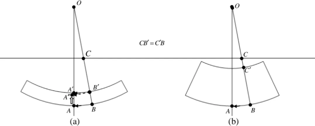
The pencil beam kernels were separated out into depth-directed and lateral components. We corrected the heterogeneity effects by scaling the depth-directed and lateral components. In typical practice, depth-directed components are corrected by moving both the interaction and calculation points (Fig. 2.1(a)). This can, however, induce some error in the spherical coordinate system. As displayed in Fig. 2.1(a), calculation point A must, in fact, be moved to point A'', not point A', when interaction point B is moved to point B', due to the arc length and curvature of AB not being equal to the arc length and
curvature of A'B'. For the AAA algorithm [26], point A'' is replaced, in an imprecise manner,
with point A' by multiplying arc length AB with a scaling factor. In order to avoid this lack of precision, we proposed moving the beamlet entry point on the surface and maintaining the point A and B positions fixed, as displayed in Fig. 2.1(b).
For the depth-directed component, therefore, function IDSS was corrected by moving
the beamlet entry point on the surface, thus achieving the DSS variation for the given beamlet. The new DSS value was computed as follows:
SSD' = pz – deff(P), (2.10)
where P is the path from the beamlet entry point to interaction point p'. The depth-directed component was corrected by using the DSS' kernel. The depth-directed component also required scaling by the local electron density, with the correction for the depth-directed component thus given as:
) ( ) ( ) (p = p p′ ′ S′ z DSS′ z w DS I I ρ , (2.11)
where IDSS' is the depth-directed component for the DSS' kernel and ρw(p') is the relative
electron density at interaction point p'.
The computation of lateral components was conducted in a similar fashion. The B C B C ′= ′ O O A′ B′ A B A B C C′ A′′ (a) (b) C
Figure 2.1 Two different manners for correcting tissue heterogeneities: (a) changing the
position of interaction point B, (b) moving the entry point C to point C' and changing the SSD of the beamlet.
energy released at interaction point p' was transported and deposited on the spherical shell
at depth pz. The effective radius r' was calculated by following collapsed path C(p) from
interaction point p' to calculation point p on the given spherical shell. The
heterogeneity-corrected lateral component kDS′ S′(r,pz) was thus expressed as follows:
) ( ) , ( ) , ( pz DSS pz w p S DS r k r k′ ′ = ′ ′ ρ , (2.12)
where kDSS' is the lateral component for the DSS' kernel and r' is the effective radius
computed as r'=deff(C(pz)). Compared with the AAA algorithm, our proposed method does
not require the effective radius to be multiplied with a scale factor owing to the depth-directed correction method we used.
The heterogeneity-corrected energy distribution from a single beamlet was calculated as the multiplication of a depth-directed component (Eq. (2.11)) with a lateral component (Eq. (2.12)): ) , ( ) ( ) ( IDSS z kDSS r z E p = ′ ′ p ′ ′ p . (2.13)
The total energy deposited into a grid point p is the integral of the contributions from the individual beamlets over the broad beam area:
∫∫
=
S
tot E dS
E (p) (p) , (2.14)
where S is the set of all beamlets. The “collapsed cone” method [42] was applied for the
superposition of the contributions from all individual beamlets. In our experiments, it was assumed that the energy released at the interaction point was transported into eight equal angular sectors, over which the superposition was performed. With respect to the x-axis of the spherical coordinate system, the cone axis directions were 0°, 45°, 90°, 135°, 180°, 225°, 270°, and 315° for the eight angular sectors, respectively.
Given that the absorbed dose is defined as the imparted energy per unit mass, the dose to a point at x in the Cartesian coordinate system is given by:
))) ( ( det( ) ( ) ( ) ( x x p x M J E D w tot ρ = , (2.15)
where J is the Jacobian of M and p=M(x) is the corresponding position in the modified spherical coordinates for the point at x. In order to decrease the error caused by the coordinate transform between these two coordinate systems, we applied the linear interpolation algorithm for the purposes of calculating the energy deposited at a point p.
In this study, we commenced by obtaining the pencil beam kernel by means of an MC simulation in the Cartesian coordinate system. This kernel was then re-sampled into the modified spherical coordinate system by applying the different sampling methods. These sampling methods differed in terms of the assumed source positions, resulting in different DSSs, and corresponded to the kernels of different DSSs. Each sampling method can be used in order to estimate the dose deposited at a certain point from the given beamlet. In this way, heterogeneities can be corrected by selecting a kernel of a special DSS, thus avoiding changes in interaction and calculation point positions (Fig. 2.1). The pencil beam kernels are not the same for different DSSs in the modified spherical coordinate system. We modeled kernels of DSS values ranging from 90cm to 115cm. The sampling interval of DSS value was 0.25cm. After obtaining the DSS value, a nearest-neighbor interpolation algorithm was applied to determine the corresponding kernel.
II.4. Dose calculation acceleration using FFTC
In order to calculate dose distributions with fast transform techniques, depth
information IDSS(p)cDSS, i(p) was separated from lateral information in Eq. (2.8). This
allowed for the total energy deposited on the shell at depth pz to then be directly obtained
by performing the Inverse Fast Fourier Transform (IFFT) of the sum of FFTC, as described below:
{
}
=∑
= = + − − 6 1 , 1 1 2 2 ) ( ) ( ) ( N i u i i SSD SSD tot y x i e F c I F F E p p p p p µ . (2.16)II.5. Validations of dose calculation methods: comparison with AAA
and MC methods
In order to assess our proposed methods, dose distributions were calculated in similar
synthetic phantoms to those used by Tillikainen et al. [26], namely (1) a water phantom, (2)
a lung slab phantom consisting of a water phantom with a 15cm slab of lung (ρw=0.3g/cm3),
(3) a bone slab phantom consisting of a water phantom with a 5cm slab of bone
(ρw=1.85g/cm3), (4) a lung block phantom consisting of a water phantom with a
10cm-thick block of lung positioned 2cm off the central axis (CAX), and (5) a bone block phantom consisting of a water phantom with a 5cm-thick block of bone positioned 2cm off the CAX.
A source-to-phantom distance of 1000mm was used for all field sizes and phantoms. The source model used in the calculations was only the primary source, since our study primarily sought to model the primary beam. We modeled dose distributions for a 6MV photon beam. The 6MV photon beam spectrum was obtained from the EGS4 Spectra
Library (file mohan6.spectrum [43]). Our proposed pencil beam model (superposition
method in Sec. II.2 and FFTC method in Sec. II.3) had been evaluated by comparing depth-dose curves and cross profiles with results obtained from using the AAA and MC
methods in the test phantoms for different photon fields. The DOSXYZnrc [44, 45] radiation
transport code was applied for MC dose calculations. The following parameters were set for the simulation: grid size=0.5cm, ECUT=0.70MeV (electron/positron minimum transport energy), and PCUT=0.01MeV (photon minimum transport energy). One billion particle histories were simulated for each experiment in order to maintain a statistical standard uncertainty of under 0.2% for an overall statistical uncertainty. The AAA algorithm we chose to employ was implemented by modeling the method proposed by
Tillikainen et al. [26]. Both the proposed method and the AAA algorithm calculated the
dose distributions in a spherical coordinate system. For our proposed method, all the voxels
exhibited the same arc length (in Eq. (2.2)), namely ∆ =0.5cm, on each spherical shell,
whereas the sampling angle was fixed (in Eq. (2.1)) for the AAA method at θ0 =0.29°. The
spherical shell thickness was 0.5cm for these two methods. Finally, all dose distributions
II.6. Results
II.6.1. Water phantom
0 50 100 150 200 250 300 20 40 60 80 100 Depth(mm) P e rc e n t d e p th d o s e (% ) 0 50 100 150 200 250 300-8 -6 -4 -2 0 2 4 6 8 D if fe re n c e (% ) Sup AAA FFTC MC AAA-MC Sup-MC FFTC-MC -50 0 50 0 10 20 30 40 50 60 70 Lateral distance(mm) R e la ti v e d o s e (% ) -50 0 50 -8 -6 -4 -2 0 2 4 6 8 D if fe re n c e (% ) Sup AAA FFTC MC AAA-MC Sup-MC FFTC-MC 0 50 100 150 200 250 300 20 40 60 80 100 Depth(mm) P e rc e n t d e p th d o s e (% ) 0 50 100 150 200 250 300-8 -6 -4 -2 0 2 4 6 8 Di ff e re n c e (% ) Sup AAA FFTC MC AAA-MC Sup-MC FFTC-MC -100 -50 0 50 100 0 10 20 30 40 50 60 70 Lateral distance(mm) R e la ti v e d o s e (% ) -100 -50 0 50 100 -8 -6 -4 -2 0 2 4 6 8 D if fe re n c e (% ) Sup AAA FFTC MC AAA-MC Sup-MC FFTC-MC
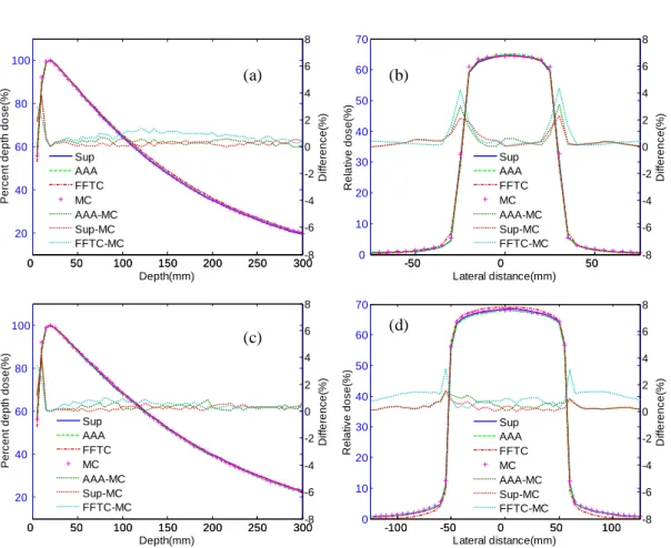
In the water phantom, we considered depth-dose curves for 50×50 and 100×100mm2
field sizes, as well as for corresponding lateral dose profiles at 100mm depth. Figure 2.2 displays the depth-dose curves and lateral dose profiles calculated by means of the superposition method, the FFTC method, the AAA algorithm, and the MC method. The results revealed that the superposition method was more accurate than the AAA algorithm and FFTC method. The mean absolute deviations of the superposition method were 0.31% and 0.34% for depth-dose curve, and 0.41% and 0.33% for lateral dose profiles, respectively for the two fields. The largest differences recorded in the calculated profiles were approximately 2.30% and 1.48%, respectively for the two fields, around the field edges. As we can infer from Fig. 2.2 (b) and (d), the accuracy of lateral dose profiles was
Figure 2.2. Water phantom: comparison of the superposition method (Sup), FFTC method
(FFTC), AAA algorithm, and MC simulation. Solid lines represent results calculated using Sup, dashed lines represent results using AAA, dashed and dotted lines represent results using FFTC, and ‘plus’ symbols represent results using MC. Dotted lines correspond to the absolute
difference between two calculation methods. (a) Depth-dose curves of 50×50mm2 field sizes,
(b) profiles at 100mm depth of 50×50 mm2 filed size, (c) depth-dose curves of 100×100mm2
field size, and (d) profiles at 100mm depth of 100×100mm2 filed size.
(a) (b)
improved by increasing the field sizes for the superposition method. The electronic disequilibrium on the field central axis reduced in size as the field size increased, thus rendering it easier to calculate dose distributions with rectilinear kernel scaling approaches and improving dose calculation accuracy. For the FFTC method, mean absolute deviations were 0.84% and 0.56% for depth-dose curves, and 0.62% and 1.09% for lateral dose profiles, respectively for the two fields. For all phantoms considered in our study, comparisons have been summarized in Table 2.1 for superposition method, FFTC method, and AAA algorithm. Our proposed method could not fully correct the build-up effects near the interfaces where the dose would jump abruptly to a new equilibrium level. Significant maximum deviations in depth-dose curves were still observed in the build-up region, estimated at 3.80% and 3.96% for AAA algorithm, 3.72% and 4.05% for the superposition method, and 2.96% and 3.43% for the FFTC method, respectively for these two fields. We can see in Fig. 2.2 (a) and (c) that, as the field size increased, accuracy decreased for the depth-dose curves in the build-up region. The pencil beam kernel was incapable of satisfactorily taking build-up effects into account. The larger the field size, the more pencil beam kernels were considered for dose calculations, which increased the number of errors occurring in the depth-dose curves in the build-up region.
Depth curves Lateral curves
Water Lung slab Bone slab Water Lung block Bone block
AAA 0.37% 1.59% 0.83% 0.48% 1.72% 0.88%
Superposition 0.34% 0.83% 0.48% 0.33% 0.94% 0.57%
FFTC 0.56% 2.89% 1.05% 1.09% 1.89% 1.08%
II.6.2. Lung slab phantom
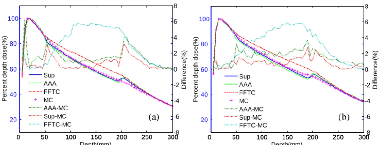
In the lung slab phantom, we calculated the depth-dose curves for the 50×50 and
100×100mm2 field sizes. Depth-dose curve comparisons are presented in Fig. 2.3. The
superposition method accurately modeled the attenuations in the lung-equivalent material, as the mean absolute deviations for these two fields were 0.73% and 0.83%, respectively for the two fields. Compared to the AAA algorithm, the superposition method reduced mean absolute deviations by 0.77% and 0.75% for these two fields, respectively. Nevertheless, the interface effects were slightly overestimated, leading to large dose deviations near the heterogeneity boundary of approximately 3.15% and 2.73%, respectively for the two fields. Owing to a neglect of density changes in lateral direction for the FFTC method, significant mean absolute deviations were observed for depth-dose curves, namely 2.85% and 2.89%.
Table 2.1. Mean absolute deviations for the AAA algorithm, superposition method, and
FFTC method for depth curves in water, and lung and bone slab phantoms, as well as lateral
curves in water, and lung block and bone block phantoms, respectively, for 100×100mm2
0 50 100 150 200 250 300 20 40 60 80 100 Depth(mm) P e rc e n t d e p th d o s e (% ) 0 50 100 150 200 250 300-8 -6 -4 -2 0 2 4 6 8 D if fe re n c e (% ) Sup AAA FFTC MC AAA-MC Sup-MC FFTC-MC 0 50 100 150 200 250 300 20 40 60 80 100 Depth(mm) P e rc e n t d e p th d o s e (% ) 0 50 100 150 200 250 300-8 -6 -4 -2 0 2 4 6 8 D if fe re n c e (% ) Sup AAA FFTC MC AAA-MC Sup-MC FFTC-MC
II.6.3. Bone slab phantom
Depth-dose curve comparisons pertaining to the bone slab phantom are presented in
Fig. 2.4 for the 50×50 and 100×100mm2 field sizes. For the superposition method, the
mean absolute deviations of depth-dose curves were 0.83% and 0.48%, respectively for the two fields, in comparison with 1.01% and 0.83% for the AAA algorithm. We also reported a slight overestimation caused by the interface effects, which resulted in deviations of approximately 2.13% and 1.54% near the heterogeneity boundary. For the FFTC method, the mean absolute deviations of depth-dose curves were 1.39% and 1.05% for these two fields, respectively. The maximum deviations observed with the FFTC method were 4.99% and 3.58% near the heterogeneity boundary.
0 50 100 150 200 250 300 20 40 60 80 100 Depth(mm) P e rc e n t d e p th d o s e (% ) 0 50 100 150 200 250 300-8 -6 -4 -2 0 2 4 6 8 D if fe re n c e (% ) Sup AAA FFTC MC AAA-MC Sup-MC FFTC-MC 0 50 100 150 200 250 300 20 40 60 80 100 Depth(mm) P e rc e n t d e p th d o s e (% ) 0 50 100 150 200 250 300-8 -6 -4 -2 0 2 4 6 8 D if fe re n c e (% ) Sup AAA FFTC MC AAA-MC Sup-MC FFTC-MC (b) (a)
Figure 2.3. Lung slab phantom: comparison of the superposition method (Sup), FFTC
method (FFTC), AAA algorithm, and MC simulation. (a) Depth-dose curves of 50×50mm2
field sizes; (b) depth-dose curves of 100×100mm2 field size.
(a) (b)
Figure 2.4. Bone slab phantom: comparison of the superposition method (Sup), FFTC
method (FFTC), AAA algorithm, and MC simulation. (a) Depth-dose curves of 50×50mm2
II.6.4. Lung and bone block phantoms
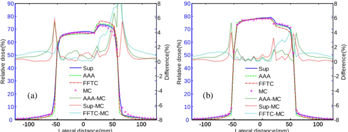
For the lung and bone block phantoms, Fig. 2.5 displays the lateral dose profiles for a
100×100mm2 field at a different depth from the phantom surface. The superposition
method accurately accounted for attenuations around the lateral material interface for both block phantoms. Mean absolute deviation was 0.94% at 100mm depth in the lung block phantom and 0.57% at 75mm depth in the bone block phantom. The maximum differences for the calculated profiles occurred near the heterogeneity boundary and around the field edges. For these two dose profiles, the largest deviations were 5.93% and 3.95% near the heterogeneity boundary and around the field edges, respectively for the two phantoms, yet remained under 1% in the other regions. Compared with the AAA algorithm, the superposition algorithm exhibited good agreement with the MC simulations, with the accuracy improving from 0.31% to 0.76% in different heterogeneous phantoms (Table 2.1). The FFTC method, which did not take into account the density changes in the lateral direction, could not accurately model the attenuations in the heterogeneities. The result was mean absolute deviations of approximately 1.89% and 1.08% for these two phantoms, respectively. -100 -50 0 50 100 0 10 20 30 40 50 60 70 80 90 Lateral distance(mm) R e la ti v e d o s e (% ) -100 -50 0 50 100 -8 -6 -4 -2 0 2 4 6 8 D if fe re n c e (% ) Sup AAA FFTC MC AAA-MC Sup-MC FFTC-MC -100 -50 0 50 100 0 10 20 30 40 50 60 70 80 90 Lateral distance(mm) R e la ti v e d o s e (% ) -100 -50 0 50 100 -8 -6 -4 -2 0 2 4 6 8 D if fe re n c e (% ) Sup AAA FFTC MC AAA-MC Sup-MC FFTC-MC 100×100 mm2 200×200 mm2 FFTC 4.0 s 4.1 s Superposition 159.8 s 182.3 s AAA 170.8 s 184.4 s MC 12 h 14 h
Figure 2.5. Lung and bone block phantoms: comparison of the superposition method (Sup),
FFTC method (FFTC), AAA algorithm, and MC simulation for 100×100mm2 field size. (a)
Profiles at 100mm depth in lung block phantom; (b) profiles at 75mm depth in bone block phantom.
(a) (b)
Table 2.2. Computational time with the FFTC method, superposition method, AAA
II.6.5. Computation time
The computational times have been presented in Table 2.2. All methods were performed on the same computer (dual-core Intel (R) Core (TM) 2 CPU 6600 platform with 2-GB memory). The run time of the computer implementation of the superposition
method came to approximately 159.8 seconds (s) and 182.3s for the 100×100 and
200×200mm2 field sizes, respectively. Dose calculations took only 4.0s and 4.1s for
64×64×60 points for these two fields with the FFTC method.
II.7. Discussion
This study has presented a new pencil beam model aimed at addressing the kernel tilting issue and accounting for heterogeneities. The superposition and FFTC methods were employed for dose distribution calculation. The results (Fig. 2.2-2.5) have revealed that the superposition method performed better than the AAA algorithm, achieving mean absolute deviations <1% in comparison with the MC method. Nevertheless, large deviations of up to 6% were detected with this method near the field edges and heterogeneous media boundary (Fig. 2.5) due to the electronic disequilibrium. The superposition method was accelerated by the FFTC technique, which is about 40 times faster (Table 2.2), yet, compared to the MC calculations, the differences observed in interface regions were significant (up to 8%). This proves that the accuracy was markedly decreased.
It should also be noted that a similar strategy for pencil beam dose calculations has
been adopted by several authors for treatment planning systems [25, 26]. In their algorithms,
the primary beam’s oblique incidence was modeled by kernels derived from the beamlets of different incident angles. In contrast, the pencil beam kernels in our proposed model were only modeled once by an MC simulation for the beamlet-normal to surface. The depth-directed components were scaled by moving the entry point’s position on the phantom surface and changing the DSS value. As opposed to the method with the AAA algorithm, therefore, the corrections for lateral components were here implemented by using density scaling directly along the spherical shell, without taking density changes in the previous layers into account. More accurate results could be obtained by modeling the beamlet around the central axis in each direction, though this would be more demanding in terms of the memory space required to store the parameters used in dose calculations.
To speed up dose calculations, significant computation time can be saved by performing FFTC calculations on spherical shells without taking into account the density changes in the lateral direction. In heterogeneous tissue, the depth-directed components can be corrected according to the interaction points. As a result, in a spherical coordinate system, the energy released at the same depth is deposited on the same spherical shell. The dose distributions in a phantom can be calculated directly on each spherical shell by means of the FFTC technique. The FFTC technique accelerated the superposition method and saved on computation time, proving approximately 40 times faster than the superposition method (Table 2.2), though accuracy was markedly decreased. Compared
to other FFTC-based methods [35, 46], our proposed method calculated dose distributions in a spherical coordinate system, avoiding the bias caused by oblique kernels. Improved dose calculation accuracy was also achieved (<3% for mean absolute deviations) compared to other FFTC-based methods reported in the literature (up to 10% for the
maximum deviations) [35, 46, 47].In IMRT systems, iterative optimization can be completed
in a reasonable time by using hybrid dose calculation methods, in which the FFTC-based method is used for most of the dose calculations, with result correction conducted by
means of a periodically updated dose correction matrix [48, 49].
In terms of computational efficiency, the superposition method achieved better calculation speeds than the AAA algorithm, though this effect was very small, as presented in Table 2.2. For hybrid-dose calculation methods in IMRT systems, significant time can be saved by using the FFTC algorithm without reducing optimization quality.
II.8. Conclusion
In this study, we have proposed a new pencil beam model aimed to avoid the bias caused by oblique kernels and to take heterogeneities into account. Our proposed method achieved better dose calculation accuracy without increasing computational time compared to the AAA algorithm. Significant computation time savings can be gained by performing FFTC calculations on spherical shells without taking density changes from the previous layers into account. Nevertheless, the accuracy was greatly decreased with this method (up to 3.0% for mean absolute deviations), as compared to the superposition method. Owing to the lack of cylindrical symmetry for the oblique beamlets, small errors may be introduced into the calculations by correcting the heterogeneous tissue with the symmetrical kernel of different DSSs, yet dose calculations are more accurate with our proposed method. In this study, the spectrum of 6MV photon beams was taken into account in calculating dose distributions in the phantom. Future studies will be focused on modeling the beam for a linear accelerator and conducting dose calculation in patients. This dose calculation process is not the only crucial part of the Treatment Planning Systems. This calculation is repeated at each iteration of an optimization process during which the plan characteristics (or the fluence map) are refined to minimize a cost function incorporating constraints on both the target and the organs at risk. The incorporation of biological constraints, namely NTCP constraints, is the purpose of the following chapter.