HAL Id: tel-00764519
https://tel.archives-ouvertes.fr/tel-00764519
Submitted on 13 Dec 2012HAL is a multi-disciplinary open access
archive for the deposit and dissemination of sci-entific research documents, whether they are pub-lished or not. The documents may come from teaching and research institutions in France or abroad, or from public or private research centers.
L’archive ouverte pluridisciplinaire HAL, est destinée au dépôt et à la diffusion de documents scientifiques de niveau recherche, publiés ou non, émanant des établissements d’enseignement et de recherche français ou étrangers, des laboratoires publics ou privés.
Solid Transport in Urban Area
Jiong Zhang
To cite this version:
Jiong Zhang. Experimental and Numerical Investigations of Flow and Solid Transport in Urban Area. Mécanique des fluides [physics.class-ph]. INSA de Rennes, 2012. Français. �tel-00764519�
Experimental and
Numerical Investigations
of Flow and Solid
Transport in Urban Area
Thèse soutenue le 13.03.2012
devant le jury composé de :
Abdelhak AMBARI
Professeur à l’E.N.S.A.M. d’Angers / président
Didier MAROT
Maître de Conférences HDR à l’I.U.T. de Saint-Nazaire / rapporteur
Nicolas LECOQ
Maître de Conférences HDR à l’Université de Rouen / rapporteur
Keld Rømer RASMUSSEN
Professeur à l’Université d’Aarhus, Danemark / examinateur
Alexandre VALANCE
Directeur de Recherche à l’Université de Rennes 1 / examinateur
Pascal DUPONT
Maître de Conférences à l’I.N.S.A. de Rennes / Co-encadrant
Mustapha HELLOU
Professeur à l’I.N.S.A. de Rennes / Directeur de thèse
THESE INSA Rennes
sous le sceau de l’Université européenne de Bretagnepour obtenir le titre de DOCTEUR DE L’INSA DE RENNES
Spécialité : Génie Civil
présentée par
Jiong ZHANG
ECOLE DOCTORALE : SDLM LABORATOIRE : LGCGM
Experimental and Numerical Investigations
of Flow and Solid Transport
in Urban Area
Jiong ZHANG
1
Acknowledgments
This work has been done in the Laboratoire de Génie Civil et Génie Mécanique (LGCGM) of the Institut National des Sciences Appliquées de Rennes (INSA de Rennes). I would like to express my gratitude to my directeurs de la recherché, Prof. Mustapha HELLOU and MCF Pascal DUPONT for their inspiration, guidance, encouragement and friendship during the course of this work. Working with them has been a rewarding and enjoyable experience. As a recipient of China Scholarship Council (CSC) scholarship I want to thank CSC for the financial support, and the Education Section of the Chinese Embassy in France for their help and kind attention.
I also wish to express my appreciation to the rapporteurs, MCF-HDR Didier MAROT and MCF-HDR Nicloas LECOQ, and all the members of the committee, Prof. Abdelhak AMBARI, Prof. Keld Rømer RASMUSSEN, and Prof. Alexandre VALANCE, for their valuable comments and review of this dissertation.
Special appreciation is extended to M. Jean-Jacques KERMAREC, the technical personal in laboratory of Géosciences Rennes, Mme. Nathalie CHOLLET the secretary of our laboratory, Dr. Guoqing JING and Dr. Boumedienne BENMEZROUA, who used to work in laboratory of LGCGM for their help and encouragement.
I would also like to thank the secretariat de l’Ecole doctorale for their help, encouragement and kind attention.
I would also like to thank all Ph.D. students from the laboratory: Amphone VONGVIXAY, Thai-Hoa NGUYEN, Soksan CHHUN, Baghdad KROUR, Sovanvichet LIM, Nhan-Hoa NGUYEN, Son-Tung PHAM, Ty SOY, Khac Chien THAI …
Also, I would like to thank all my friends from INSA de Rennes: Dr. Cunsheng ZHANG, Dr. Pengcheng MU, Dr. Fan SUN, Dr. Hui BIAN, Dr. Ming LIU, Dr. Xiao BAI, Dr. Fen ZHOU, Yanyan CAO, Yun LUO, Cong BAI, Xing-Rong CHU, Shunying ZHANG, Linning PENG, Jinglin ZHANG … for their encouragement and friendship.
Finally, my deepest gratitude goes to my parents, for their forever support and love. You are always who I can count on, and you will always be.
1
Chapter 1 Introduction ... 7
1.1 General background... 7
1.2 Objectives of this research ... 8
1.3 Structure of thesis ... 8
Chapter 2 Literature Review of Particle Transport ... 11
2.1 Introduction ... 11
2.2 A brief review of pipe flow and open channel flow ... 11
2.2.1 Pipe flow ... 12
2.2.2 Open channel flow ... 15
2.3 Flow over and within the saturated porous medium ... 18
2.4 Critical velocity for particle erosion ... 21
2.5 The transport of sediment particles ... 24
2.6 Sediments clogging in the porous medium... 29
Chapter 3 Numerical Method... 31
3.1 Introduction ... 31
3.2 Computational Fluid Dynamics (CFD) ... 32
3.2.1 Governing equations ... 32
3.2.1.1 Law of mass conservation ... 33
3.2.1.2 Law of conservation of momentum ... 33
3.2.1.3 Energy equations ... 33
3.2.2 Standard k-ε model ... 33
3.2.3 Numerical analysis method ... 34
3.2.3.1 Discretization method ... 34
3.2.3.2 Derivation of algebraic equations ... 36
3.2.3.3 Under-relaxation ... 38
3.2.4 Volume of Fluid (VOF) method ... 38
2
3.3.2 Time-step ... 41
3.3.3 Damping ... 41
3.3.4 Contact Model ... 42
3.4 CFD and DEM two-way coupling ... 43
3.5 Validation test of the method ... 45
3.6 Conclusions ... 50
Chapter 4 Experimental Method ... 51
4.1 Description of the experimental settings ... 51
4.1.1 Design of hydraulic parameters in the study ... 51
4.1.2 Flow channel ... 52
4.1.3 Water supply ... 54
4.1.4 The measure of flow rate ... 54
4.1.5 Particle adding device... 55
4.1.6 Porous bed ... 55
4.2 Measure of the particle velocity ... 58
4.3 Measure of the flow velocity field by a PIV system ... 58
4.4 Conclusions ... 62
Chapter 5 Free Surface Flow over a Porous Bed in an Open Channel ... 63
5.1 Introduction ... 63
5.1.1 Experimental setup ... 63
5.1.2 Process of the experiment ... 64
5.1.3 Numerical setup ... 65
5.2 Parameters of the study ... 65
5.3 Results and analysis ... 66
5.3.1 Raw results ... 66
5.3.2 Reference case ... 68
5.3.3 Flow regimes ... 69
3
5.3.4.2 Influence of flow rate ... 71
5.3.5 Velocity distributions above and within the porous region ... 72
5.3.5.1 Influence of channel slope ... 72
5.3.5.2 Influence of flow rate ... 74
5.3.6 Shear velocity ... 76
5.3.7 Turbulent kinetic energy above and within the porous region ... 81
5.3.7.1 Influence of channel slope ... 81
5.3.7.2 Influence of flow rate ... 83
5.4 Conclusions ... 86
Chapter 6 Particle Incipient Motion over a Porous Bed ... 89
6.1 Introduction ... 89
6.1.1 Experimental setup ... 89
6.1.2 Process of the experiment ... 90
6.1.3 Numerical setup ... 91
6.2 Parameters of the study ... 91
6.3 Results and analysis ... 92
6.3.1 Influence of channel slope ... 92
6.3.2 Influence of particle diameter ... 95
6.4 Conclusions ... 99
Chapter 7 Particle Transport over a Porous Bed ... 101
7.1 Introduction ... 101
7.1.1 Experimental setup ... 101
7.1.2 Process of the experiment ... 102
7.1.3 Numerical setup ... 103
7.2 Parameters of the study ... 103
7.3 Results and analysis ... 105
7.3.1 Raw results ... 105
4
7.3.2.2 Influence of flow rate ... 107
7.3.2.3 Influence of particle diameter ... 108
7.3.3 Analysis of particle velocity distribution along the vertical direction ... 109
7.3.3.1 Influence of channel slope ... 110
7.3.3.2 Influence of inflow rate ... 113
7.3.3.3 Influence of particle diameter ... 115
7.3.4 Analysis of particle motion in flow ... 118
7.3.5 Analysis of horizontal component of particle velocity distribution in ascent and descent motion ... 121
7.3.6 The mean vertical component of particle velocity distribution in ascent and descent motion ... 123
7.3.7 Formula for determining the velocity of particle ... 126
7.4 Conclusions ... 128
Chapter 8 Sediment Clogging Phenomenon in an Open Channel with a Porous Bed .. 131
8.1 Introduction ... 131
8.1.1 Experimental setup ... 131
8.1.2 Process of the experiment ... 132
8.2 Parameters of the study ... 133
8.3 Results and analysis ... 134
8.3.1 Sediment clogging ... 134
8.3.2 Sediment transport rate over porous bed ... 135
8.3.2.1 Influence of inflow rate ... 136
8.3.2.2 Influence of channel slope ... 139
8.3.2.3 Influence of particle diameter ... 142
8.3.2.4 Influence of seepage outflow rate ... 144
8.3.2.5 Empirical bed-load transport relation ... 145
8.4 Conclusions ... 146
Chapter 9 General Conclusions ... 149
5
9.3 Particle transport over a porous bed ... 151
9.4 Sediment clogging phenomenon in an open channel with a porous bed ... 152
9.5 Suggestions for further research ... 152
9.5.1 From experimental point of view ... 152
9.5.2 From numerical point of view ... 153
References ... 155
Appendix ... 161
7
Chapter 1
Introduction
1.1 General background
In modern society, land development can increase the amount of stormwater runoff and its associated pollutant loads to receiving waters (Barrett et al., 1998). Several authors have studied stormwater runoff carries off dissolved, colloidal and solids components from the urban surfaces (e.g. Chang and Crowley, 1993 and Ball et al., 2000).
A porous medium is a material containing large number of randomly located voids (pores) of sizes greater than the microscopic interatomic scale such as soil, rocks, sponge, etc. Transport phenomena at the interface between a fluid and porous medium has remained an important topic of research because of their fundamental interest in understanding the phenomena of infiltration into the porous medium and its wide field of applications in industry and environmental analyses, for example, urban hydrology, river hydraulics, pollution and remediation of soils, water treatment, etc.
As in urban hydrology field, the erosion and clogging phenomena of road cause a lot of economic losses and even threaten the people’s lives, because these are the results of an effect of sediment transport caused by flow after rains, a better understanding of details of flow structures near the surface of road (a kind of porous medium) will help to improve the design of road and provide optimized solutions.
8
Flows over a porous medium are the flows combined both over and through the porous medium. Because of the interaction between surface flow and seepage flow inside porous region, this interaction affects both the flow discharge and the sediment discharge.
In recent years, due to the development of the computational capacity, a complex computational fluid dynamics (CFD) could be performed. Meanwhile the discrete element method (DEM), developed by Cundall and Strack (1979), has been used extensively to investigate the behavior of granular solids subjected to a variety of loading conditions with the goal of understanding and predicting quantitative results.
1.2 Objectives of this research
The aim of this research was to study the characteristics of a free surface flow over a porous bed in an open channel and the sediment transport by this kind of flow numerically and experimentally.
A 3D CFD–DEM method was used for simulation of complicated behavior including interaction between particle and fluid in the combined domain, involving both a porous region and a clear fluid region. This methodology will have a wider application to granular solids transport in flows in general.
A series of laboratory experiments were carried out using a channel consists of a platform with supports that allow adjustment of the slope, and a layer of porous media was placed at the bottom of the channel. A Particle Image Velocimetry (PIV) system was used to obtain the flow velocity field and a high speed camera was used to capture the velocity of particles.
1.3 Structure of thesis
The thesis is divided into eight chapters. A brief outline of each chapter is described below. Chapter 1 presents the background and objectives of this research.
Chapter 2 reviews the literature relevant to this thesis. It focuses on flows over and within a porous medium and particle transport.
Chapter 3 describes numerical method used in this research. That includes the Equations of fluid dynamics, Equations of particles and CFD-DEM two-way coupling method.
Chapter 4 describes the experimental method to validate simulation results. That includes the experimental design and measuring methods.
9
Chapter 5 studies the characteristics of a free surface flow over a porous bed in an inclined open channel numerically and experimentally. Effects of the dynamic characteristics of open channel and porous bed, such as channel slope, inflow rate, and seepage outflow rate, on the free surface flow are investigated.
Chapter 6 focuses on the problem in studying critical velocity of grain over porous medium in open channel.
Chapter 7 presents the research on single particle transport in open channel over a porous bed. Effects of the dynamic characteristics of porous medium, including channel slope, inflow rate, seepage outflow rate, and particle size on the particle movement are further investigated. Chapter 8 aims at solving the problem in studying sediment clogging in open channel over a porous bed.
Chapter 9 summarizes the general conclusions of the whole thesis and makes recommendations for further work.
11
Chapter 2
Literature Review of Particle
Transport
2.1 Introduction
Sediment dynamics in geophysical flows has been the centre of a great deal of research over the last century. In recent years, because of the development of the computational capacity, complex CFD and DEM calculation could be performed to understand the phenomenon at the grain scale.
This review consists of three main parts:
• A brief review of pipe flow and open channel flow; • A review of flows over and within a porous medium; • A review of the critical velocity for particles;
• A review of the sediment transport in open channel flow; • A brief review of the particle clogging in the porous medium.
2.2 A brief review of pipe flow and open channel flow
The flow of water in a conduit may be either an open channel flow or a pipe flow. Compared with pipe flow the open channel flow differ in one important aspect that it must have a moving free surface, whereas pipe flow has none.
12
It is much more difficult to solve problems of flow in open channels than in pipes. Flow conditions in open channels are complicated by the position of the free surface which could change with time and space, and also by the fact that the depth of the flow, the discharge rate, and the slopes of the channel bottom and of the free surface are all inter dependent.
Treatment of roughness also poses a greater problem in open channels than in pipes. Although there may be a wide range of roughness in a pipe from polished metal to highly corroded iron, open channels may be of polished metal up to natural channels with long grass and roughness interacting with the flow depth.
2.2.1 Pipe flow
One of the most particular cases of flow may be laminar flow. This flow is characterized by fluid particles moving along smooth paths in laminas or layers, with one layer gliding smoothly over an adjacent layer.
In the case of laminar flow, the Hagen–Poiseuille law gives the pressure drop in a fluid flowing through a long pipe of uniform cross-section, which can be derived directly from the Navier–Stokes equation (White, 2003). The assumptions of the equation are that the flow is laminar, viscous and incompressible and that the flow passes through a constant circular cross-section that is substantially longer than its diameter. The Hagen–Poiseuille equation is: 𝑈𝑤 =∆𝐻∆𝐿𝜌𝑔𝐷𝐻
2 32𝜇
(2-1) where Uw is the mean velocity; ΔH is the head loss due to friction; DH is the pipe diameter; μ
is the viscosity of the flow; g is the gravity.
Taking the Darcy-Weisbach formula for head loss due to friction: ∆𝐻 = 𝑓𝐷Δ𝐿
𝐻 𝑈𝑤2 2𝑔
(2-2) Take (2-2) into the equation Hagen-Poisseuille (2-1), then the friction coefficient f is: 𝑓 =64
𝑅𝑒
(2-3) with the Reynolds number Re is defined as:
𝑅𝑒 =𝑈𝑤𝑣𝐷𝐻 (2-4)
The Reynolds number Re is the criterion for determining the type of flow. The limits for laminar and turbulent are:
13
Turbulent: Re > 4000
Ludwig Prandtl (1875-1953), the German genius engineer, introduced the boundary layer theory in 1904. One of his earliest students, Paul R. H. Blasius, provided a mathematical basis for boundary-layer drag and showed as early as 1911 that the resistance to flow through smooth pipes could be expressed in terms of the Reynolds number for both laminar and turbulent flows. His phenomenological formula is the first correlation ever made for the turbulent pipe flow, between the friction factor and the Reynolds number:
𝑓 =0.3164𝑅𝑒1/4 (2-5)
The range of application is 4000 < Re < 105 (Streeter and Wylie, 1981).
From 1931 to 1933, Johann Nikuradse performed his classical measurements in rough pipes. Nikuradse (1933) took a number of smooth pipes of diameter 2.5, 5 and 10 cm, and tightly coated the inside walls with uniform grains of graded sand. The relative roughness of each tube was then defined as ks/DH, where ks was the diameter of the sand grains and DH the
diameter of the tube. The advantages of dimensionless numbers had been well learned from Reynolds. Nikuradse took pressure drop and velocity profile measurements in the pipes and obtained the corresponding f−Re graphs which are illustrated on Figure 2-1.
Figure 2-1. The friction factor vs. Reynolds number diagram resulted from the experiments with sand-grain roughness by Nikuradse (1933). The figure is taken from Schlichting (1968) Nikuradse observed that at low Reynolds numbers the laminar friction factor correlation is valid irrespective of the grain size. However, turbulent friction correlation, after an onset point, increases monotonically with ks/DH. For any given relative roughness, the friction
14
factor eventually becomes constant at higher Reynolds numbers. Based on these observations, Nikuradse introduced the roughness Reynolds number 𝑅𝑒∗= 𝑘𝑠𝑈∗/𝑣 in order to characterize the observed behavior of turbulent flow in rough pipes.
The hypothesis of the existence of a boundary layer assisted Nikuradse to explain the behavior of the curves in Figure 2-1. At the walls, there can be no cross velocities except on a molecular scale. Hence, there must be a thin layer called sub-layer close to each wall through which the velocity increases from zero (actually at the wall) to some finite velocity sufficiently far away from the wall for an eddy to exist. Although this viscous layer is very thin, it has a marked effect on the behavior of the total flow in the pipe. All real surfaces (even polished ones) have some degree of roughness. If the peaks of the roughness do not protrude through the viscous sub-layer (Re* < 7) then the surface may be described as
hydraulically smooth and the wall resistance is limited to that caused by viscous shear within the fluid. Within the second range (7 < Re* < 70), there will be a transition zone, where an
increase in the resistance factor was observed for an increasing Reynolds number. The resistance factor depends upon both the Reynolds number and relative roughness. Within the third range (Re* > 70), the resistance factor is independent of the Reynolds number:
1
�𝑓= −2.0 𝑙𝑜𝑔10 𝑘𝑠 3.7𝐷𝐻
(2-6) Further experiments and analytical investigations to derive a resistance formula for rough pipes were carried out in England by Colebrook (1939) in the late 1930’s and followed by an engineer from Princeton, Lewis F. Moody (1944). Moody’s landmark paper appeared after those of Nikuradse and Schlichting and represented the first easily applied and universally accepted method of comparing flow resistance for fully developed flow in commercially-rough pipes.
15
Figure 2-2. Moody diagram. The figure is taken from Chanson (2004)
2.2.2 Open channel flow
As in pipes, the flow in an open channel may be either laminar or turbulent. In practice, hydraulic radius RH=DH/4 is often used for an open channel as a mean flow depth, and the
thresholds become: Laminar: Re < 500 Turbulent: Re > 1000
y
x
u
θ
d
16
Figure 2-3. Sketch of the flow over an inclined plane
Considering a viscous incompressible fluid flow over a wide inclined plane with a uniform velocity distribution, under gravity force, using the Navier–Stokes equation, we can deduce the velocity distribution along y direction as follows:
𝑢 =𝜌𝑔𝑠𝑖𝑛𝜃2𝜇 𝑦(2𝑑 − 𝑦) (2-7)
and the relation between flow rate per unit width and flow depth is:
𝑞 =𝜌𝑔𝑠𝑖𝑛𝜃3𝜇 𝑑3 (2-8)
where u is the velocity distribution along y direction, θ is the inclination angle of the plane, d is the flow depth, q is the flow rate per unit width.
The first empirical equation to calculate the energy losses in turbulent flow was given by Antoine Chézy in 1775, called Chézy equation:
𝑈𝑤 = 𝐶𝐶ℎé𝑧𝑦�𝐷4 sin 𝜃𝐻
(2-9)
where CChézy is the Chézy coefficient (units m
1/2
/s), which is not constant and expresses the importance of roughness. DH is the hydraulic diameter and θ is the channel slope (e.g.
Henderson, 1966).
Many studies have been performed for evaluating CChézy for different natural and manmade
channels. Some forms of the relationships are used by today’s engineers, one of them is known as Manning formula:
𝐶𝐶ℎé𝑧𝑦 =𝑛 1 𝑀𝑎𝑛𝑛𝑖𝑚𝑔�
𝐷𝐻 4 �
1/6 (2-10)
and Equation (2-9) becomes: 𝑈𝑤 =𝑛 1 𝑀𝑎𝑛𝑛𝑖𝑛𝑔� 𝐷𝐻 4 � 2/3 √sin 𝜃 (2-11)
where nManning is the Manning coefficient (units s/m
1/3
).
There have been several other names of this formula or ones similar and consequently in some countries the same equation is named after one of these people, some of these names are Strickler, Gauckler, Gauguillet and Hagen.
17
The Manning equation has the great benefits that it is simple, accurate and use extensively since a long time. There are different values of nManning for a wide range of open channels.
Table 2-1 gives a list of a few typical values of Manning coefficient. Table 2-1. Typical values of Manning coefficient Channel type Surface material and form nManning range
River earth, straight 0.02-0.025 earth, meandering 0.03-0.05 gravel (75-150mm), straight 0.03-0.04 gravel (75-150mm), winding 0.04-0.08 Unlined canal earth, straight 0.018-0.025
rock, straight 0.025-0.045 Lined canal concrete 0.012-0.017 Lab. models mortar 0.011-0.013
Perspex 0.009
The shear velocity is a measure of shear stress and velocity gradient near the boundary, a large shear velocity U* implies large shear stress and large velocity gradient. Generally, there
are four methods to estimate the shear velocity: Reynolds stress, logarithmic law, parabolic law and a global approach.
The logarithmic law method is based on the velocity distribution in the region y/d<0.6, can be described by the logarithmic law: 𝑢
𝑈∗=
1 𝜅ln(
𝑦
𝑘𝑠) + C, where κ is the von Karman constant
(equal to 0.41), and C is a constant.
Einstein and El-Samni (1949) proposed a modified logarithmic law for the flow over a surface with large roughness: 𝑢
𝑈∗=
1 𝜅ln(
𝑦+𝑦0
𝑘𝑠 ) + C, where y0 is the distance of the theoretical
wall below the top of the spheres whose diameter is ks, they chose a value of y0=0.2ks.
Cheng and Chiew (1998) suggested a modified logarithmic law for the influence of vertical seepage flow: 𝑢 𝑈∗= 1 𝜅ln( 𝑦 𝑦0) + 𝑉𝑠 4𝑈∗( 1 𝜅ln 𝑦 𝑦0) 2, where V
s is the vertical mean seepage flow rate
18
2.3 Flow over and within the saturated porous medium
The first characteristic of a porous medium is the porosity measured by the porosity factor which is the ratio of volume of voids (or pores) to the total volume including both solids and voids. The porosity factor Φ for sediment bed of rivers ranges usually from 0.26 to 0.48. Another characteristic of a porous medium is the permeability. For a one-dimensional flow through the pores of the sediment bed, the velocity of seepage is given by the Darcy law:
𝑈𝑠 = 𝐾∆𝐻∆𝐿 (2-12)
where Us is the mean flow velocity in porous medium, which is also called Darcy velocity, K
is the coefficient of permeability, and ΔH is the head loss over a distance ΔL. The coefficient of permeability K not only depends on the permeability of the soil but also on the properties of the fluid and dimensional analysis yields (Raudkivi and Callander, 1976):
𝐾 = 𝑘𝑝𝜌𝑔𝜇 (2-13)
where kp is the intrinsic permeability (in m
2
), ρ is the fluid density, g is the gravity constant and µ is the fluid dynamic viscosity. The intrinsic permeability depends only on the structure of the porous medium. Typical values of the coefficient of permeability are given in Table 2-2 (Raudkivi and Callander, 1976):
Table 2-2. Typical values of the coefficient of permeability Soil type Fine sand Silty sand Silt
K (m/s) 5×10⁻⁴ to 1×10⁻⁵ 2×10⁻⁵ to 1×10⁻⁶ 5×10⁻⁶ to 1×10⁻⁷
Darcy law is no longer validated when the permeability is large or velocity is large. Moreover the Darcy law could just get the mean flow velocity across the section of porous media, but could not describe the details of the flow structure in the pores.
Li and Garga (1998) presented analytical results for the turbulent seepage flow occurring at the transition zone (between the fluid zone and the pressure seepage zone) of gravel river reaches or nonconventional rockfill spillways. They proposed an approach based on analyses between porous media and pores network. The flow velocity in the pores Uv may be defined
as:
𝑈𝑣 =𝑈𝛷𝑠 (2-14)
19
The Darcy-Weisbach formula expressed the friction coefficient: 𝑓 =∆𝐻∆𝐿2𝑔𝐷𝐻𝛷2
𝑈𝑠2
(2-15) Based on experiments, Hansen (1992) concluded that the friction coefficient is linked with Reynolds number like:
𝑓 = 𝑎
𝑅𝑒 + 𝑏 (2-16)
where a, b are coefficients. Hence, the Reynolds number Re may be written as: 𝑅𝑒 =𝑈𝑣𝐷𝐻
𝑣 = 𝑈𝑠𝐷𝐻
𝑣𝛷
(2-17) The Equation (2-16) could be used in both laminar and turbulent flows. The constant coefficient b is negligible for small Reynolds number and Equation (2-16) is changed into Poisseuille’s law. When Reynolds number increases f tends to be a constant value of b, and the stability of f is a characteristic of the turbulent flow in porous media.
The combination of Equations (2-15), (2-16) and (2-17) lead to a general equation of flows over and in porous medium:
∆𝐻 ∆𝐿 = 𝑎𝜐 2𝑔𝐷𝐻2𝛷𝑈𝑠+2𝑔𝐷𝑏 𝐻𝛷2𝑈𝑠 2 (2-18)
The flow phenomena and momentum transfer at the porous/fluid interface have also been studied by several investigators. Beavers and Joseph (1967) used a porous block with high permeability in a closed channel in their experimental study, and found an empirical relationship for the interfacial slip velocity. The empirical relationship used is
𝑑𝑈𝑤 𝑑𝑦 =
𝛼
�𝑘𝑝(𝑈𝑖𝑛𝑡− 𝑈𝑠)
(2-19) where kp is porous medium permeability; α is slip parameter; Uw is flow velocity over the
porous surface: Uint is interfacial velocity; and Us is Darcy velocity within the porous bed.
They used the momentum equation for fully developed laminar flow and the above mentioned relationship as an interfacial condition for calculating: (i) the velocity distribution over the porous media; (ii) the interfacial velocity Uint; and (iii) the increase in mass flow over the
permeable bed with regard to that with an impermeable bed.
Poulikakos and Kazmierczak (1987), Rudraiah (1985), and Vafai and Thiyagaraja (1987) used the Navier-Stokes equations for the flow above the porous medium and the Darcy equations for the flow in the porous medium. They used continuity conditions at the interface for both velocity and shear stresses, calculated the interfacial velocity and the velocity distribution above and inside the porous region.
20
Sahraoui and Kaviany (1992) showed that a variable viscosity should be used in the Darcy-Brinkman equations for an accurate calculation of the velocity near the interface and inside the porous layer. Ochoa-Tapia and Whitaker (1995a, b) have developed a stress jump condition based on the nonlocal form of the volume averaged Stokes equations and explored the use of a variable porosity model as a substitute for the jump condition. This approach did not successfully represent of all experimental data, but provided an insight into the complexities of the interfacial region between a porous medium and a free flow.
Choi and Waller (1997) applied a macroscopic single domain approach to treat complex interaction of the flow near the interfacial region. The flow was laminar and the results showed the importance of viscous shear in the channel flow. They concluded that the Darcy law is inappropriate to be used in the interfacial region.
James and Davis (2001) used microscopic models for Stokes flow in a channel partially filled with an array of circular cylinders. The porosity was 0.9 or greater, simulating fibrous porous media. They concluded that the external flow penetrates the porous layer very little even for sparse arrays and that the apparent slip velocity at the interface is about one quarter of the velocity predicted by the Brinkman model.
Zippe and Graf (1983), based on experimental findings, found that the boundary resistance of the tested permeable surface is higher than that of the non-permeable boundary with same roughness.
Shimizu et al. (1990) based on experimental findings, concluded a mathematical model of the velocities within the porous medium under turbulent flow, However, the model was based on a function of the slip interfacial velocity, which is not known a priori. Thus, applying such a model is rather difficult. Mendoza and Zhou (1992) and Zhou and Mendoza (1993) presented the turbulent flow characteristics over a porous bed and the velocity distribution in surface flow, however, the details of transport phenomena near the boundary of the permeable interface was not investigated.
Hahn et al. (2002) applied direct numerical simulation (DNS) to the fluid region only for turbulent flow conditions. They found a significant skin-friction reduction at the permeable wall, a decrease of the viscous sub-layer thickness, and a weakening of the near-wall vortices. Either microscopic or macroscopic model can be used in the numerical investigation of the turbulent flow over the porous region. Most of the studies on porous medium flow apply macroscopic models within a two-dimensional (2D) porous bed. Pedras and de Lemos (2000) presented a macroscopic turbulent model which was a k-ε model based on the formulations
21
developed from the numerical results. Chan et al. (2007) presented the numerical solutions for turbulent 2D flow in a channel with a porous medium, they applied a single-domain approach and concluded that the level of turbulent penetration depends strongly on the damping effect of the porous medium itself. However using the macroscopic models could not have detailed insight into the flow structure. Hence, due to the development of the computational capacity, a complex computational fluid dynamics (CFD) could be performed. Prinos et al. (2003) presented microscopic computation of flow over and within a porous bed. They also provided very valuable measured data.
2.4 Critical velocity for particle erosion
It is important to understand the mechanism of sediment incipience for investigating sediment transport.
For an open channel flow with a porous bed, the forces acting on each sediment particle are shown in Figure 2-4.
• The gravity force ρsgΩs;
• The buoyancy force Fb =ρgΩs;
• The drag force CdρAsUw 2
/2; • The lift force CLρAsUw
2
/2;
• The inter-granular forces (contact forces).
where Ωs is the volume of the particle, As is a characteristic particle cross-sectional area, Cd
and CL are the drag and lift coefficients, respectively, Uw is a characteristic flow velocity next
22 Uw Lift force Buoyancy force Drag force Gravity force
Figure 2-4. Forces acting on a sediment particle (inter-granular forces not shown for the purpose of clearness)
The gravity force and the buoyancy force act both in the vertical direction while the drag force acts in the flow direction and the lift force in the direction perpendicular to the flow direction (Figure 2-4). The inter-granular forces are related to the grain disposition and packing.
There is a sediment transport when the force acting on particles is big enough for moving them, so the sediment transport is a phenomenon with a threshold. The threshold of sediment motion cannot be defined with an exact precision but most experimental observations have provided reasonably accurate and consistent results.
The relevant parameters for the analysis of sediment transport threshold are: the bed shear stress τo, the sediment density ρs, the fluid density ρ, the grain diameter ds, the gravity
acceleration g and the fluid viscosity µ:
𝑓1(𝜏0; 𝜌; 𝜌𝑠; 𝜇; 𝑔; 𝑑𝑠) = 0 (2-20a)
In dimensionless terms, it yields: 𝑓2�𝜌𝑔𝑑𝜏0 𝑠; 𝜌𝑠 𝜌 ; 𝑑𝑠�𝜌𝜏0 𝜇 � = 0 (2-20b)
Introducing the shear velocity U* defined as:
𝑈∗= �𝜏𝜌0
(2-21)
23 𝑈∗= �𝑔𝐷4 𝑠𝑖𝑛𝜃𝐻
(2-22)
Equation (2-20) can be changed into: 𝑓3� 𝑈∗ �𝑔𝑑𝑠; 𝜌𝑠 𝜌 ; 𝜌 𝑑𝑠𝑈∗ 𝜇 � = 0 (2-20c)
The first term is in a form of the Froude number. The second is the relative density. The last term is a shear Reynolds number or particle Reynolds number.
In 1936, Shields introduced a dimensionless parameter τ* called the Shields parameter,
defined as: 𝜏∗=(𝜌 𝜏0
𝑠− 𝜌)𝑔𝑑𝑠
(2-23) A critical value of this parameter (τ*)c may be defined at the inception of bed motion.
Shields (1936) showed that (τ*)c is primarily a function of the shear Reynolds number V*ds/v
(Figure 2-5).
Figure 2-5. Shields diagram: Shields parameter as a function of the particle Reynolds number for sediment in water
For sediment particles in water, the Shields diagram exhibits different trends corresponding to different turbulent flow regimes:
• The smooth turbulent flow (Re* < 5) 0.035< (τ*)c;
• The transition regime (5< Re* < 70) 0.03< (τ*)c < 0.04;
24
For fully rough turbulent flows, the critical Shields parameter (τ*)c is nearly constant, and
the critical bed shear stress for bed load motion becomes linearly proportional to the sediment size:
(τo )c ∝ds Fully rough turbulent flow (2-24)
The inception of bed load motion may be affected by several parameters: particle size distribution, bed slope, bed forms and material cohesion (van Rijn, 1993).
2.5 The transport of sediment particles
When the bed shear stress exceeds a critical value, sediments are transported. For bed-load transport, the basic modes of particle motion include rolling motion, sliding motion and saltation motion. Saltation refers to the transport of sediment particles in a series of irregular jumps and bounces along the bed (Figure 2-6). The sediment transport can damage the environment and destroy human infrastructure. Figure 2-7 shows the landslide in Zhouqu County in China that occurred at midnight on August 8, 2010, which has killed More than 1471 people, was caused by heavy rainfall and flooding.
Uw
Up
25 (a)
26 (c)
Figure 2-7. Landslides strike Zhouqu County, China, August 8, 2010. (a) A handout photo from the State Bureau of Surveying and Mapping shows a combo of satellite images showing Zhouqu before (left) in July, 2008 and after the recent landslide (right), taken on August 8, 2010. (b) An aerial view of the town of Zhouqu shortly after a deadly flood-triggered landslide, seen on August 8, 2010. (c) Chinese rescuers search for survivors in the aftermath of a landslide. (Xinhua Images)
Krumbein (1942) studied the effect of particle shape on sediment transportation based on experiments. He related the observed behavior to the settling velocities of particles. The experiments were confined to the bed movement of single particles of different shapes, over a hydraulically smooth bed, for turbulent flow. He found a relationship between sphericity and the ratio of particle velocity to mean flow velocity, Up/Uw, as a function of the Froude
number. 𝑈𝑝 𝑈𝑤 = � 𝑈𝑝 𝑈𝑤�0�1 − exp (−𝑏𝐹𝑟)� (2-25) where Up is the particle velocity; Uw is the mean flow velocity; b is a constant parameter; Fr
27
Kalinske (1942) reported that the Froude number Fr has no physical significance in regard to the movement of particles on the bed. Kalinske proposed that the particle velocity should be related to critical velocity of the particle. Kalinske concluded the following expression:
𝑈𝑝= 𝑐𝑎(𝑈𝑤− 𝑈𝑐) (2-26)
where ca: constant parameter; Uc: critical velocity for a particle. Kalinske used his model
and Krumbein’s data found the best agreement for 0.9< ca<1.0.
Einstein (1950) suggested that the particle velocity in the bed-load motion is equal to 11.6 times of shear velocity (Up=11.6U*).
Ippen and Verma (1955) analyzed the motion of particles in turbulent flow over fixed beds of different roughness in flume experiments. They found that after a transition of variable length, Uw/Up reached a constant value over a wide range of Re and that the particle velocity
increased directly with size, and related this to the fact that larger particles are exposed to higher flow velocity. They obtained the following equation:
𝑈𝑤 𝑈𝑝 = 1 + 1 12 � 𝜌𝑠 𝜌 − 1� � 𝑘𝑠 𝑑𝑠� � 1 �𝑆𝑜� (2-27) where ρs/ρ: the relative density of grains; ds: particle diameter; ks: roughness size; So: slope
of energy gradient.
Meland and Norrman (1966) studied the interactive effects of water velocity, bed roughness, and particle size on the transport rate of single particles over rough beds by turbulent flows, keeping particle shape, density and bed packing constant. They explained the phenomena of larger particles move faster than smaller ones for a given bed roughness and shear velocity, First, larger particles ride higher off the bed, being thus exposed to greater velocities, and second, the rolling resistance decreases when the ratio of particle size to roughness size is increased. They also concluded that at high shear velocities and small bed roughness, the particle velocity tends to be constant with size. They also found that transport velocities were higher on beds of tightly packed solid beds than in corresponding loosely packed glass beads. But this effect was most noticeable at high transport stages, and decreased, or even reversed for low shear velocities.
Ikeda (1971) studied theoretically the mechanics of the motion of a single spherical grain rolling on the bed, by considering the four main forces acting on the particle: drag, lift, gravity and friction with the bed. The resulting particle velocity is as follows:
28 𝑈𝑝 𝑈∗ = 𝑈𝑤 𝑈∗ − � 4 3 𝑐𝜇 �𝜌𝑠 𝜌 − 1� �𝑐𝜇𝐶𝐿+ 𝐶𝑑� 𝑔𝑑𝑠 𝑈∗2� 1/2 (2-28)
where U*: shear velocity; cµ: sliding friction coefficient; Cd and CL: the drag and lift
coefficients respectively.
Bagnold (1973) assumed the particle velocity equals to the difference between flow velocity at corresponding water depth and settling velocity of particle: Up=U-w0.
Francis (1973) studied the motion of a single grain rolling on the bed. The experiments were conducted in which heavy solid grains are observed as they are propelled one at a time by a water stream over a fixed, plane, bed of grains of the same sort.. Francis found a satisfactory correlation between the particle velocity, Up and the particle settling velocity, w0.
He also concluded that rounded particles always roll faster than angular ones.
Jan (1992) studied the relative contribution of the stresses developed in granular fluid flows. Jan determined how much each of the examined stresses contributed to the total stress acting on a rolling sphere. Experiments were conducted for the steady movement of a sphere rolling down smooth and rough inclined surface in air, water and salad oil. An equation was derived expressing the velocity of a sphere rolling down a rough incline without acceleration or deceleration based on the principle of conservation of momentum. The average terminal velocity Up was derived as follows:
𝑈𝑝= �(𝜌𝑠− 𝜌)𝑔𝑑𝑠�sin 𝜃 − 𝑛𝜇cos 𝜃� 𝑓𝑐𝜌𝑠+ 34𝐶𝑑𝜌
(2-29)
where ρs, ρ: particle and fluid densities; Cd: drag coefficient; θ bed slope angle; fc:
coefficient of restitution (0.667); and nµ: bulk friction coefficient (0.13). Both fc and nµwere
determined from experimental data. The tested particle was identical to those comprising the roughness over which it rolled in Jan’s experiments. Roughness particles were tightly spaced in a single layer on a smooth wooden bed of a tilting flume. Jan found that velocity is independent of rolling particle density; collision stresses increase with increased bed inclination.
Bigillon (2001) conducted an experiment in an inclined, narrow, glass-sided channel, 2m in length and 20 cm in height. The channel inclination angle ranged from 0° to 12°. Two types of spherical particles (glass beads and steel beads, with the density of 2500 and 7750 kg/m3respectively) were used in the experiments. The water supply at the channel entrance was controlled by an electromagnetic flow meter. The flow depth was a few particle
29
diameters. The channel bed was made up of regularly disposed half-cylinders of equal size. Bigillon used three sizes of cylinder with a radius of 1.5 mm, 3 mm, and 4 mm. A single particle was dropped from above into the water stream 1 m upstream from the measuring window. The motion of mobile beads was recorded using a high speed camera. For each flow condition (Uw, θ), the variability of the results was evaluated by repeating the run between
three and five times, and only the average value was reported. The standard deviation was low relative to the mean (less than 5%) when the particle rolled. Fifty experimental data points were collected and the variability for hydraulic and particle parameters include: the range of shear velocity U*= 0.018-0.038 m/s, particle diameter ds= 1.5 mm and 3 mm, ρs/ρ = 2.5
(glass bead) and 7.75 (steel bead), ks= 1.5 mm and 3 mm, bed slope So = 0.02 and 0.05, mean
flow velocity Uw= 0.223-0.492 m/s, flow depth d = 2.13-28.65 mm, and observed bed-load
particle velocity Up= 0.076-0.496 m/s.
2.6 Sediments clogging in the porous medium
When the sediment transport capacity is smaller in the channel, the sediments transported by fluid will deposit and small particles attempt to percolate through the porous medium. When the size or concentration of small percolating particles is too large, clogging of pores can occur which can modify the permeability of the crossed medium. The literature on the sediments clogging phenomena in channel flows is hard to find, but the transport of small spherical particles through packings of larger spheres in vertical system has already been studied both experimentally and numerically.
Nguyen (2007) studied experimentally the sediment transport into porous medium. Based on the structure of road, Nguyen developed a model of porous media using two layers of glass particles placed in a transparent tank with a regulation value at the bottom. The upper layer is 5 cm thick, made up by 4 mm glass particles, and the porosity is 0.3; the lower layer is 10 cm thick, made up by a mixture of 12 mm and 15 mm glass particles, and the porosity is 0.31. First, the porous media is saturated by water. Second, use the regulation value to keep the initial water depth drop at 1 mm/s, lay the sand with diameters from 0.1 to 0.5 mm evenly on the surface of the porous medium. Then, the saturate with water till the initial level, and start a series of 10 cycles of drainage and refill. For studying the influence of surface status, silicone oil was also used to soak the porous media before the saturation of water. According to the observations, Nguyen concluded that the increase of mass of sand laid on the surface of porous media could decreases of infiltration rate, and the decrease could be enhanced because of oil soak; the oil soaked sand penetrate less deeply into the porous media than the clean sand because of the adhesion force.
30
Remond (2010) studied numerically the percolation of small particles (with a diameter of 1 cm) through a periodic random loose packing of large beads (with a diameter of 10 cm) with Distinct Element Method (DEM). Results show that a steady state is rapidly reached where the mean velocity and mean vertical velocity of small particles are both constant. These mean velocities decrease with an increase in friction coefficient and in small particle concentration. This influence is much less evident for the friction coefficient values larger than or equal to 0.5. The distribution of small particles throughout the crossed packing becomes rapidly heterogeneous. Small particles concentrate in some pores where the density can reach values larger than the density of the random loose packing. The proportion of particles blocked in these pores varies linearly with concentration. The narrow throats of the porous medium responsible for blocking are identified. And increasing the friction coefficient leads to an increase in the number of clogged pores.
Haselbach (2006) studied both theoretically and experimentally runoff on a permeable concrete block. A relation between the permeability of the sand-clogged pervious concrete block system, the porosity of the block near the surface and the permeability of the sand was established as follows:
𝐾𝑒𝑓𝑓 = 𝛷𝑡𝑜𝑝𝐾 (2-30)
where Keff: the permeability of the sand-clogged pervious concrete block; Φtop: the porosity
of the block near the surface; K: the permeability of the sand. Permeability was then measured for pervious concrete systems fully covered with extra fine sand in a flume using simulated rainfalls. Two different slopes (2% and 10%) were used. Rainfall rates were simulated for the combination of direct rainfall and for additional stormwater runoff from adjacent areas. A computer-monitored scale was used to record the change in weight of the runoff water collected over time. The concrete block was approximately 31 cm in length, 31 cm in width and 16 cm in depth with a surface area of 948 cm2. The block was placed on self compacted 15 cm thick sand which in turn was placed on a perforated wooden board wrapped with a layer of geo-synthetic filter able to contain the sand. This entire set-up was inside a plastic container with a drainage hole at the bottom. To simulate a varying range of sand clogging, wet sand was placed over the block at three different depths (1.3, 2.5 and 5 cm). The sand was also distributed over the flume surface for an additional 30 cm upslope of the block to minimize channeling effects at the flume/pervious interface. The experimental results correlated well with the calculated permeability of the pervious concrete system fully covered on the surface with sand.
31
Chapter 3
Numerical Method
3.1 Introduction
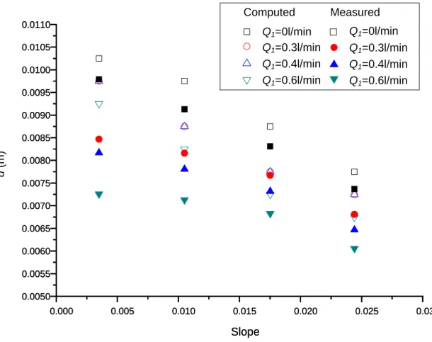
The characteristics of a free surface flow over a porous bed in a three-dimensional (3D) inclined open channel are investigated using a microscopic approach. Figure 3-1 shows the flow investigated here. The rectangular channel is partially filled with a layer of porous material. A free surface flow passes longitudinally from left to right. At the bottom, the seepage outflow rate can be controlled.
Free flow Interface Free surface Inclination angle Inflow rate: Q Wall Outflow rate: Q2 H L Porous region θ d hp Seepage outflow rate:
Q1
Figure 3-1. Sketch of computational domain with boundary conditions in a 2D view In this chapter the numerical methods applied in the study are introduced. For this objective, a combination of Computational Fluid Dynamics (CFD) and Discrete Element Method (DEM) is used to simulate the behavior including interaction between particles and fluid. The governing equations are solved using the commercial software PFC3D 4.0 (2008) and CCFD
32
(2007). In order to validate the results obtained by the CFD-DEM coupling, we compare them to the results of two test cases from literatures:
- The flow in a porous medium studied experimentally by Shimizu et al. (1990).
- The turbulent flow in the fluid over the porous medium studied both experimentally and numerically by Prinos et al. (2003).
3.2 Computational Fluid Dynamics (CFD)
The history of CFD started in the early 1960’s. Around that time, it became an acronym for a combination of physics, numerical mathematics, and to some extent, computer sciences employed to simulate fluid flows. Since the early 1970s, commercial computer codes became available, making CFD an important component of engineering practice. With the beginning of the 1980’s, the solution of first two-dimensional and later also three-dimensional Euler equations became feasible. With the mid 1980’s, the focus started to shift to the significantly more demanding simulation of viscous flows governed by the Navier-Stokes equations. Together with this, a variety of turbulence models evolved with different degree of numerical complexity and accuracy. Nowadays, CFD methodologies are routinely employed in the fields of aircraft, turbo-machinery, car and ship design. Furthermore, CFD is also applied in environment, meteorology, oceanography, geotechnics, and in oil recovery, etc...
3.2.1 Governing equations
The three laws governing the fluid motion are the following: 1. The law of conservation of mass (transport of mass); 2. Newton’s second law of motion (transport of momentum); 3. The first law of thermodynamics (transport of energy).
Governing equations are described by integral expressions using control volume Ω surrounded by surface area S, a surface element as dS and its associated, outward pointing unit normal vector 𝑛�⃗ as shown in Figure 3-2. In addition, 𝑉�⃗Rs here is the transfer velocity of the boundary. When 𝑉�⃗Rs is the same as velocity 𝑉�⃗ of the continuum, the equations of motion are described by a Lagrangian form and when 𝑉�⃗Rs = 0, they are described by an Eulerian form.
33 i3 x3 i1 i2 dS P Ω r Vs x2 x1 n
Figure 3-2. Control volume
3.2.1.1 Law of mass conservation
The mass conservation law is known as the equation of continuity and is represented by the following equation.
𝑑
𝑑𝑡 � 𝜌𝑑𝛺𝛺 + � 𝜌�𝑉�⃗ − 𝑉�⃗𝑆 𝑠�∙ 𝑛�⃗𝑑𝑆 = 0 (3-1) where dS is the surface element.
3.2.1.2 Law of conservation of momentum
By means of applying Newton’s second law to the control volume of Figure 3-2, the following equation known as Cauchy’s first law of motion is derived.
𝑑
𝑑𝑡 � 𝜌𝑉𝛺 �⃗𝑑𝛺+ � 𝜌𝑉�⃗�𝑉�⃗ − 𝑉�⃗𝑆 𝑠� ∙ 𝑛�⃗𝑑𝑆 = � 𝜏̿ ∙ 𝑛�⃗𝑑𝑆 + � 𝑓⃗𝑆 𝛺 𝑏𝑑𝛺 (3-2) where 𝜏̿ is a Cauchy stress tensor and 𝑓⃗Rb is the volume force per unit volume.
3.2.1.3 Energy equations
𝑑
𝑑𝑡 � 𝜌𝐸𝑑𝛺𝛺 + � 𝜌𝐸�𝑉�⃗ − 𝑉�⃗𝑆 𝑠� ∙ 𝑛�⃗𝑑𝑆 = � 𝑞⃗𝑆 ℎ∙ 𝑛�⃗𝑑𝑆 +� s𝛺 ℎ𝑑𝛺
(3-3) Where E is the total energy per unit mass, 𝑞⃗Rh is a heat flux vector and sh is a heat source.
3.2.2 Standard k-
ε model
The standard k-ε model is often used to model turbulent flow. Turbulent kinetic energy k and eddy dispersion rate ε are modeled by the following transport equations.
34 𝑑 𝑑𝑡 � 𝜌𝑘𝑑𝛺 + � 𝜌𝑘(𝑉𝛺 𝑆 �⃗ − 𝑉�⃗𝑆) ∙ 𝑛�⃗𝑑𝑆 = � �𝜇 +𝜇𝑡 𝜎𝑘� grad𝑘 ∙ 𝑛�⃗𝑑𝑆 + � (𝑃 + 𝑃𝛺 𝐵− 𝜌𝜀)𝑑𝛺 𝑆 (3-4) 𝑑 𝑑𝑡 � 𝜌𝜀𝑑𝛺 + � 𝜌𝜀�𝑉𝛺 𝑆 �⃗ − 𝑉�⃗𝑆�∙ 𝑛�⃗𝑑𝑆 = � �𝜇 +𝜎𝜇𝑡 𝜀� grad𝜀 ∙ 𝑛�⃗𝑑𝑆 𝑆 + � (𝐶1𝑃𝑠𝜀𝑘 + 𝐶2𝜌𝜀 2 𝑘 + 𝐶3max(𝑃𝐵, 0) 𝜀 𝑘 − 𝐶4𝜌𝜀div𝑉�⃗)𝑑𝛺 𝛺 (3-5)
where µ is the viscosity coefficient of the fluid, and the eddy viscosity coefficients µt is
represented as: 𝜇𝑡 = 𝐶𝜇𝜌𝑘
2 𝜀
(3-6) Turbulent kinetic energy generated by shear Ps and the effect due to buoyancy PB are
modeled as:
𝑃𝑠=23 (𝜇𝑡div𝑉�⃗ + 𝜌𝑘)div𝑉�⃗ (3-7)
𝑃𝐵 = −𝜌𝜎𝜇𝑡
𝑇𝑔 ∙ grad𝜌 (3-8)
where Cµ, C1, C2, C3, C4, σk, σε, σT are experimental constants and Table 3-1 shows their
values.
Table 3-1. Experimental constants in standard k-ε model
Cµ C1 C2 C3 C4 σk σε σT σci
0.09 1.44 1.92 1.44 -0.33 1.0 1.3 0.9 0.9
3.2.3 Numerical analysis method
The governing equation and the standard turbulent model can be uniformly described as follows: 𝑑 𝑑𝑡 � 𝜌𝜑𝑑𝛺 + � 𝜌𝜑�𝑉𝛺 𝑆 �⃗ − 𝑉�⃗𝑆�∙ 𝑛�⃗𝑑𝑆 = � Γ𝜑grad𝜑 ∙ 𝑛�⃗𝑑𝑆 + � 𝑞𝜑𝑆∙ 𝑛�⃗𝑑𝑆 𝑆 + � 𝑞𝛺 𝜑𝛺𝑑𝛺 𝑆 (3-9)
where φ is called conservative variables. Γφ is a diffusion coefficient of φ.
35
In order to handle values such as velocity, temperature, turbulent energy k, and eddy dispersion rate ε, discretization is performed using the format of Equation (3-9).
Generally, there are four discretization methods, finite difference method, finite element method, finite analytic method and finite volume method. In this research a finite volume method is used to perform discretization based on non-structural lattices. The advantages of using a finite volume method are shown below.
First, finite volume methods ensure that the discretization is conservative, i.e., mass, momentum, and energy are conserved in a discrete sense. While this property can usually be obtained using a finite difference formulation, it is obtained naturally from a finite volume formulation. Second, finite volume methods do not require a coordinate transformation in order to be applied on irregular meshes. As a result, they can be applied on unstructured meshes consisting of arbitrary polyhedra in three dimensions or arbitrary polygons in two dimensions. This increased flexibility can be used to great advantage in generating grids about arbitrary geometries.
The CCFD uses a collocated grid to arranged variables in center of a cell. If the symbols of Figure 3-3 are used, Equation (3-9) will be written as follows.
i3 x3 i1 i2 dS s1 P0 V rP0 sj x2 x1 P1 Pj
36 𝑑 𝑑𝑡 � 𝜌𝜑𝑑𝛺 + � � 𝜌𝜑�𝑉𝑆 �⃗ − 𝑉�⃗𝑆� 𝑛𝑓 𝑗=1 ∙ 𝛺 𝑛�⃗𝑑𝑆 = � � Γ𝜑grad𝜑 ∙ 𝑛�⃗𝑑𝑆 𝑠𝑗 𝑛𝑓 𝑗=1 + � � 𝑞𝜑𝑆∙ 𝑛�⃗𝑑𝑆 𝑠𝑗 𝑛𝑓 𝑗=1 + � 𝑞𝜑𝛺𝑑𝛺 𝛺 (3-10)
where nf is the number of surfaces comprising a cell. The first term on the left side of
Equation (3-10) is an unsteady term and the second term is and advective term. The first term on the right side is a diffusion term and the second and third terms are both source terms. The following procedure is completed in order to evaluate the integral terms appearing in Equation (3-10).
1. Shape data processing to calculate the surface integral and cubic volume integral 2. Select approximation method of cubic volume integral
3. Select interpolation method of variables
4. Select discretization method for advective terms 5. Select integral scheme
6. Calculate velocity of cell interface
3.2.3.2 Derivation of algebraic equations
A SIMPLE method has been used as a solution method of equation (3-10). The linear simultaneous equation derived when applying a SIMPLE method is as follows (Patanker, 1980).
The unsteady terms of equation (3-10) use an implicit method of first order precision to perform discretization as follows.
𝑑
𝑑𝑡 � 𝜌𝜑𝛺 𝑑𝛺 ≈
(𝜌𝜑𝛺)𝑃0− (𝜌𝜑𝛺)𝑃𝑚−10
𝛿𝑡𝑚
(3-11) where ρ is density, ϕ is a conservative variable, δtm is a time unit.
The flux of variable φ that passes through the cell surface is as follows. 𝐶𝑗= � 𝜌𝜑�𝑉�⃗ − 𝑉�⃗𝑆� ∙ 𝑛�⃗𝑑𝑆
𝑆𝑗
≈ 𝑚̇𝑗𝜑𝑗∗ (3-12)
where 𝜑𝑗∗ represents the value at the center of the surface comprising the cell and 𝑚̇𝑗 is the mass flux on the surface of the cell derived by the following equation.
37 𝑚̇𝑗= � 𝜌�𝑉�⃗ − 𝑉�⃗𝑆� ∙ 𝑛�⃗𝑑𝑆
𝑆𝑗
≈ 𝜌𝑗∗�𝑉𝑗∗∙ 𝑆𝑗− 𝑉̇𝑗� (3-13) 𝜌𝑗∗ and 𝑣𝑗∗ are the density and velocity at the cell surface.
Flux on the cell surface due to diffusion of variable φ is approximated by the following equation.
𝐷𝑗= � Γ𝜑grad𝜑 ∙ 𝑛�⃗𝑑𝑆 𝑠𝑗
≈ Γ𝜑,𝑗(grad𝜑)𝑗∗∙ 𝑆𝑗 (3-14)
where, Γφ is a diffusion coefficient on the cell surface.
The source acting on surfaces such as heat flux acting on the surface of a physical object and the source acting on cubic volume such as acceleration of gravity during heat generation or at the location of flow while performing heat transfer analysis is approximated as follows: Surface source: 𝑄𝜑𝑆= � 𝑞𝜑𝑆 𝑆 ∙ 𝑛�⃗𝑑𝑆 ≈ ⎩ ⎨ ⎧ ���𝜇𝑒𝑓𝑓(grad𝑉)𝑇− �23 𝜇𝑒𝑓𝑓div𝑉 + 𝑝� 𝐈� 𝑗∙ 𝑖𝑖� ∙ 𝑠𝑗 , for 𝜑 = 𝑉𝑖 𝑛𝑓 𝑗=1 0 , for 𝜑 = 𝑐𝑖, 𝐸, 𝑘, 𝜀 (3-15)
Cubic volume source: 𝑄𝜑𝛺= � 𝑞𝜑𝛺𝑑𝛺 ≈ �𝑞𝜑𝛺�𝑃0
𝛺 𝛺𝑃0
(3-16) From Equations (3-10) to (3-16), Equation (3-9) becomes a linear equation using the value of φ at the center of the cell and the value φ at the adjacent cell. It can be written as follows:
𝑎𝜑0𝜑𝑃0− � 𝑎𝜑𝑗𝜑𝑃𝑗
𝑛𝑓
𝑗=1
= 𝑏𝜑 (3-17)
where each term is calculated as: 𝑎𝜑𝑗 = Γ𝜑𝑗 𝑠𝑗∙ 𝑠𝑗 𝑑𝑗∙ 𝑠𝑗− min (𝑚̇𝑗, 0) (3-18) 𝑎𝜑0 = � 𝑎𝜑𝑗+ (𝜌𝛺)𝑃𝑚−10 𝛿𝑡𝑚 𝑛𝑓 𝑗=1 (3-19)
38 𝑏𝜑 = � Γ𝜑𝑗�(grad𝜑)𝑗∙ 𝑆𝑗− 𝑔𝑟𝑎𝑑𝜑��������� ∙ 𝑑𝑗 𝑆𝑗∙ 𝑆𝑗 𝑑𝑗∙ 𝑆𝑗� 𝑛𝑓 𝑗=1 − �𝛾2 𝑚̇𝜑 𝑗��𝑟𝑗− 𝑟𝑃0� ∙ (grad𝜑)𝑃0+ �𝑟𝑗− 𝑟𝑃𝑗� ∙ (grad𝜑)𝑃𝑗 𝑛𝑓 𝑗=1 + �𝑟𝑗− 𝑟𝑃𝑗� ∙ (grad𝜑)𝑃𝑗� + 𝑄𝜑𝑆+ 𝑄𝜑𝛺 + � 𝑎𝜑𝐵+ (𝜌𝛺𝜑)𝑃𝑚−10 𝛿𝑡𝑚 𝑛𝐵 𝐵=1 (3-20)
where nb=nf - ni is the number of boundaries.
A SIMPLE algorithm uses the following procedure:
1. Uses an already known value to form and linearize coefficient matrix 𝑎𝜑𝑗 and source term 𝑏𝜑 for Equation (3-17). The linear simultaneous equation of this result is derived:
𝐴𝜑𝜑 = 𝑏𝜑 (3-21)
where Aφ is a matrix of N × N. Vector φ is a dependent variable vector in the center of N
number of cells and bφ is a source vector.
2. Equation (3-21) is solved for each dependent variable. Because each coefficient matrix and the right side are approximated using the previous step value at this time, solving this equation is not strictly required.
3. Repeats until steps 1 and 2 are a predetermined convergence error.
3.2.3.3 Under-relaxation
When Equation (3-21) is calculated, variations in the values will increase rapidly often making it impossible to perform stable calculations. Because of this, the CCFD transforms the coefficient matrix and right side vector of Equation (3-21) as shown below:
𝐴𝜑 → 𝐴𝜑+1 − 𝛽𝛽 𝜑
𝜑 𝐷𝜑 , 𝑏𝜑→ 𝑏𝜑+
1 − 𝛽𝜑 𝛽𝜑 𝐷𝜑𝜑
𝑘−1 (3-22)
where 𝛽𝜑 is a relaxation coefficient and is a value between 0 and 1, 𝐷𝜑 is a diagonal term of matrix 𝐴𝜑 and 𝜑𝑘−1 is a value before one step of the reiteration process.
3.2.4 Volume of Fluid (VOF) method
A method used for advecting an interface is the volume of fluid method originally developed by Hirt and Nichols (1981). This method uses a fluid fraction variable F, which varies between 0 and 1, indicating the fraction of each computational cell that is filled with a fluid
39
phase. This VOF function F is then advected according to the local flow velocity. More accurate schemes for advecting the volume fractions have been developed after that. A comprehensive review is given by Rider and Kothe (1998). Generally, there are two classes of methods, namely piecewise constant and piecewise linear reconstructions of the interface, dependent on the required accuracy of the interface and the reconstruction.
3.3 Discrete Element Method (DEM)
DEM is a popular numerical technique for computing the behavior of discrete particles. This method was originally applied by Cundall (1971) to problems in rock mechanics. The method is based on the use of an explicit numerical scheme in which the interactions between a finite number of particles are monitored contact by contact and the motion of the particles is modeled particle by particle. Each contact follows a soft contact approach where an overlap of particles is accepted. This overlap is not a real phenomenon but instead intends to model the deformation of the interacting bodies at a contact point in an indirect way. The particles are treated as rigid bodies and the overlap during a contact is assumed to be relatively small compared to the particle size.
The DEM scheme relies upon the assumption that a small enough time step should be chosen to ensure that, during a single time step, others disturbances do not propagate from any particle further than its immediate neighbors. DEM has the capacity of modeling materials at microscopic levels and analyzing multiple interacting bodies undergoing large displacements and rotations, thus capturing all the phenomena that relates to the particulate nature of granular media. Following the pioneering work of Cundall and Strack (1979), research into DEM has increased dramatically in light of its potential.
3.3.1 Particles movement
The force-displacement law is used to find contact forces from known (and fixed) displacements, the Newton’s second law gives the motion of the particles resulting from the known (and fixed) forces acting on them. The Figure 3-4 presents the calculation cycle scheme.
40
Figure3-4. DEM calculation cycle scheme
The solid movements are determined by writing Newton’s dynamic relations. The motion of a single rigid particle is determined by the resultant force and moment vectors acting upon it, and can be described in terms of the translational motion of a point in the particle and the rotational motion of the particle. The translational motion of the center of mass is described in terms of its position, xi, velocity, 𝑥̇𝑖, and acceleration, 𝑥̈𝑖; the rotational motion of the particle
is described in terms of its angular velocity, ωi, and angular acceleration, 𝜔̇𝑖. The
corresponding equations that describe translation and rotation of the particle about its center of mass are developed as:
𝑚𝑥̈𝑖 = �� 𝐹𝑖𝑐 𝑁𝑐 𝑐=1 � + 𝑚𝑔𝑖 (3-23) 𝐼𝜔̇ = � 𝑀𝑖𝑐 𝑁𝑐 𝑐=1 (3-24) where m is the mass of the particle, Nc is the number of contacts, 𝑥̈𝑖 is acceleration of the
solid centroid, 𝐹𝑖𝑐 and gi are the ith components of the contact force F and the gravity g, I is
the inertia of the block, 𝜔̇ is the angular acceleration of the solid centroid, 𝑀𝑖𝑐 is moment of
ith particle.
In order to solve the Newton’s equations in a discrete way, the DEM describe the translational and rotational accelerations at time t in terms of the velocity values at mid-intervals. The accelerations are calculated as: