NUMERICAL SIMULATION OF TURBULENT FLOW UPSTREAM OF THE
INCEPTION POINT IN A STEPPED CHANNEL
S. BENMAMAR & A. KETTAB & C. THIRRIOT
Département Hydraulique, Laboratoire LRS-Eau, Ecole Nationale Polytechnique 10, Avenue Hassen Badi B.P. 182, El Harrach, Alger Algerie
e-Mail : benmamar@yahoo.fr
ABSTRACT
From the crest of the chute or from the upstream gate, a bottom turbulent boundary layer develops. We present a numerical model of the two dimensional flow boundary layer in stepped channels with steep slope, which is based on the implicit finite difference scheme.
From the mass and linear momentum conservation equation taking into account characters of the boundary layer, a system of non linear parabolic equations governing the flow has been developed. The turbulence stresses are closed by using k-ε model.
A discrete system of equation has been obtained. By allowing to calculate the velocity profile, water surface profiles, the boundary layer thickness and position of inception of air entrainment. The latter has been determined as intersection of the boundary layer and the free surface.
A numerical model is presented to analyse the location of the start of air entrainment and the variables of the flow (velocity, turbulent kinetic energy, turbulent kinetic energy dissipation and turbulent viscosity).
Keywords: Boundary layer – Stepped channel - Free surface - 1. INTRODUCTION
On a stepped spillway with skimming flow, the entraining region follows a region where the flow over the spillway is smooth and glassy. Next to the boundary however turbulence is generated and the boundary layer grows until the outer edge of the layer reaches the surface (figure 1).
Figure 1 : Definition sketch h l d Growing boundary layer hc Non –aereted flow region Gradually varied flow Uniform flow region ° ° ° ° ° ° ° ° ° ° ° ° ° ° ° ° ° ° ° ° ° ° ° ° ° ° ° ° ° ° ° ° ° ° ° ° ° ° ° ° ° Point of inception XI α E I Limit of calculation procedure
When the outer edge of the boundary layer reaches the free surface, the turbulence can initiate natural free surface aeration (Chanson, 1994). The location of the start of air entrainment is called the point of inception. A statistical analysis of the data indicates that the flow properties are best correlated by :
(
)
( )
(
)
( )
° α ° ⎪ ⎪ ⎭ ⎪⎪ ⎬ ⎫ α = α α = α for 27 53 F sin 4034 , 0 cos d d F sin 72 , 9 cos d X 6 , 0 * 04 , 0 I 7 , 0 * 08 , 0 I p p in which :(
)
3 * cos d sin g q F α α =in which XI, distance from the start of growth of boundary layer to the inception point of air
entrainment, dI flow depth at the inception point, F*, Froude number, d, height of step and α,
channel slope (figure 1).
In this study, a numerical model is developed for simulating the two-dimensional flow boundary layer in stepped channels with steep slope. The distribution of the velocity as wellas the thickness of the boundary layer can be determined for every section of the channel and permit the calculation of the water line and the position of the point of inception.
2. MATHEMATICAL MODEL
Lane (1939), Hickox (1945) and Halbronn (1952, 1953) showed that the phenomenon of air entrainment begins from the point where the boundary layer reaches the free surface.
The flow on a stepped channel, can be simulated as flow of an incompressible viscous fluid on a rough profile and governed therefore by the equations of conservation of the mass and momentum, based on the theory of the boundary layer (Schlichting, 1968) and the following hypotheses: The channel is considered large; The liquid is supposed incompressible (the fluid density is constant); The out-flow is turbulent; The out-flow is considered steady; The distribution of pressure is hydrostatic.
Equations representing the flow may be written:
(
)
y ' v ' u y u x P 1 g.sin y u v x u u 2 2 ∂ − ∂ + ∂ ∂ ν + ∂ ∂ ρ − α = ∂ ∂ + ∂ ∂ (1)(
α ρ = g y.cos P)
(2) (I) 0 y v x u = ∂ ∂ + ∂ ∂ (3)in which u and v = mean velocity components in the x and y direction respectively; u’ and v’ = velocity fluctuation components; ρ = density; µ = viscosity; P = the pressure, and g sin α = the component of gravitational acceleration along the spillway face.
The system (I) can be solved only if the Reynolds stress is known. By assuming a form analogous to that for laminar shear stress −u'v', may be expressed as
(
)
y u 1 ' v ' u t ∂ ∂ µ ρ = − , in
which the eddy viscosity : µ =ρ µ ε 2 t C k .
(
)
−ε ∂ ∂ − + ⎟⎟ ⎠ ⎞ ⎜⎜ ⎝ ⎛ ∂ ∂ µ ∂ ∂ ρ + ⎟ ⎟ ⎠ ⎞ ⎜ ⎜ ⎝ ⎛ ∂ ∂ σ µ ∂ ∂ ρ = ∂ ∂ + ∂ ∂ y u ' v ' u y k y 1 y k y 1 y k v x k u k t (4)(
)
k C y u k C ' v ' u y y 1 y y 1 y v x u 2 t 2 1 ε − ∂ ∂ ε − + ⎟⎟ ⎠ ⎞ ⎜⎜ ⎝ ⎛ ∂ ε ∂ µ ∂ ∂ ρ + ⎟ ⎟ ⎠ ⎞ ⎜ ⎜ ⎝ ⎛ ∂ ε ∂ σ µ ∂ ∂ ρ = ∂ ε ∂ + ∂ ε ∂ ε ε ε (5)in which, k turbulent kinetic energy, ε turbulent kinetic energy dissipation. The values of empirical constants are (Launder and Spalding, 1974) : Cµ = 0.09;Cε1=1.43;Cε2= 1.92; σk =
1.0; σε=1.30
The similarity among equations leads to the following general form of the equation to be
solved : φ φ + ⎟⎟ ⎠ ⎞ ⎜⎜ ⎝ ⎛ ∂ φ ∂ µ ∂ ∂ ρ + ⎟ ⎟ ⎠ ⎞ ⎜ ⎜ ⎝ ⎛ ∂ φ ∂ σ µ ∂ ∂ ρ = ∂ φ ∂ + ∂ φ ∂ S y y 1 y y 1 y v x u t (6) 3. NUMERICAL MODEL
The flow domain can be divided into two regions : From the spillway bed (I boundary) to the boundary layer edge (E boundary) ; and from E boundary to the free water surface.
Following the numerical method of Patankar and Spalding, equation (6) has been modified from the x-y to the x-ω, in which, ω is the nondimensionalised stream function
E I ψ−ψ ψ
−
ψ . From the definition of stream function,
dx d m I I ψ − = & and dx d m E E ψ − = & (7)
in which and = rates of mass transfer across the I and E boundaries, respectively. Using equations (3) and (7), the conservation equation (6) can be written as follows :
I m& E m&
(
)
( )
( )
φ φ + ⎟⎟ ⎠ ⎞ ⎜⎜ ⎝ ⎛ ω ∂ φ ∂ ψ ∆ ρ µ ω ∂ ∂ + ⎟⎟ ⎟ ⎠ ⎞ ⎜⎜ ⎜ ⎝ ⎛ ω ∂ φ ∂ ψ ∆ σ ρ µ ω ∂ ∂ = ω ∂ φ ∂ ψ ∆ ω + ω − + ∂ φ ∂ S' u u m m 1 x 2 2 t E I & & (8) in which : u S S′φ = φ and ∆ψ=ψE −ψI In the present problem m 0I =
& , equation (8) may be written in the form:
( )
( )
⎪ ⎪ ⎪ ⎪ ⎩ ⎪⎪ ⎪ ⎪ ⎨ ⎧ ε − ⎟ ⎠ ⎞ ⎜ ⎝ ⎛ ω ∂ ∂ ψ ∆ ρ + ⎟ ⎠ ⎞ ⎜ ⎝ ⎛ ω ∂ ε ∂ ω ∂ ∂ + ⎟ ⎠ ⎞ ⎜ ⎝ ⎛ ω ∂ ε ∂ ω ∂ ∂ = ω ∂ ε ∂ + ∂ ε ∂ ε − ⎟ ⎠ ⎞ ⎜ ⎝ ⎛ ω ∂ ∂ ψ ∆ ρ ε + ⎟ ⎠ ⎞ ⎜ ⎝ ⎛ ω ∂ ∂ ω ∂ ∂ + ⎟ ⎠ ⎞ ⎜ ⎝ ⎛ ω ∂ ∂ ω ∂ ∂ = ω ∂ ∂ + ∂ ∂ ∂ ∂ ρ − α + ⎟ ⎠ ⎞ ⎜ ⎝ ⎛ ω ∂ ∂ ω ∂ ∂ + ⎟ ⎠ ⎞ ⎜ ⎝ ⎛ ω ∂ ∂ ω ∂ ∂ = ω ∂ ∂ + ∂ ∂ ε µ ε ε ω µ ω ω u . k C u . u k C C e C b x u u . u k C k e k C k b x k x P . u 1 sin u g u e u C u b x u 2 2 2 2 2 2 2 2 k u 2 1 (9) in which : ψ ∆ = mE b & ,( )
2 t. .u C φ ∆ σ ρ µ = φ φ and( )
2 u . . e ψ ∆ ρ µ =Applying equation (9) for the velocity beyond the E boundary, where there are no gradients in the cross-stream direction, we obtain :
u S x u ∂ = ′
∂ (10)
Now it is assumed that equation (10) is applicable just inside the E boundary also, with the result that equation (9) may be written as :
NE u . b ω ∂ ∂ ω = NE u u C ⎟ ⎠ ⎞ ⎜ ⎝ ⎛ ω ∂ ∂ ω ∂ ∂ (11)
gradients in finite difference form, the following expression for b is obtained : NE E NE u E u u u u C u C b − ⎟ ⎠ ⎞ ⎜ ⎝ ⎛ ω ∂ ∂ − ⎟ ⎠ ⎞ ⎜ ⎝ ⎛ ω ∂ ∂ = (12)
3.1 IMPLICIT FINITE DIFFERENCE SCHEME
The numerical scheme used in this study is based on an implicit finite difference scheme :
(
) ( )
x j , i j , 1 i x ∆ φ − + φ = ∂ φ ∂ (13)(
) (
)
ω ∆ + φ − + + φ = ω ∂ φ ∂ i 1,j 1 i 1,j (14)(
) (
)
( ) (
)
(
) (
)
( )
2 1 j , 1 i . 1 j , i C j , 1 i . j , i C 2 1 j , 1 i . 1 j , i C C ω ∆ − + φ − + + φ − + + φ + = ⎟ ⎠ ⎞ ⎜ ⎝ ⎛ ω ∂ φ ∂ ω ∂ ∂ φ φ φ φ (15)(
) (
)
( ) (
)
(
) (
)
( )
2 1 j , 1 i . 1 j , i d j , 1 i . j , i e 2 1 j , 1 i . 1 j , i e e ω ∆ − + φ − + + φ − + + φ + = ⎟ ⎠ ⎞ ⎜ ⎝ ⎛ ω ∂ φ ∂ ω ∂ ∂ (16) 3.2 INITIAL CONDITIONSTo start the computations, the values of all dependent variables have to be specified at all the grid points.
• The analysis of the data indicates that, in both cases, the velocity distribution follows a power law: n / 1 l y U u ⎟ ⎠ ⎞ ⎜ ⎝ ⎛ δ
= , in which: Ul free stream velocity, δ, boundary layerthickness, y, the
ordinate of the point consideredand n=κ 8f , where κ, Karman constant, f, friction factor.
• In addition to initial data of discharge and depth at the spillway crest, the model requires an estimate of the boundary layer thickness at the crest; Following the method of Henderson (1966) : ⎟, in which δ ⎠ ⎞ ⎜ ⎝ ⎛ = δ − 30. d d
initial H 0.0055 .h initial is the boundary layer thickness at the crest; 755
. 0 h
Hd = c , design head on spillway crest (Hickox, 1945).
• The initial profile for k was obtained from equation (Huang, Kawahara and Tamai, 1993):
( )
(
2 2 l 0.08 0.08 y U k = − δ)
(17)• The initial profile for ε was obtained from equation, ε=Cµk32 l, in which the turbulence length, l, was determined from the following distribution (Schlichting, 1968):
y 42 . 0 l= for 42 . 0 09 . 0 y < δ , l=0.09 δ for 42 . 0 09 . 0 y ≥ δ
3.3 PROFILE OF THE FREE SURFACE
The profile of the free surface can be determined by the differential equation of gradually varied flow in a uniform channel as follows:
(
)
(
)
[
3]
C 3 D E dx I 1 h h 1 h h h d = − − (18)where, hE is the height of the flow, I the slope of the channel, hD the normal depth and hC the
critical depth.
With reference to figure 1, the boundary condition are : U = Ul in which Ul the free stream
velocity and Ul
(
−∂Ul ∂x)
=gsin α, k = 0; ε = 0 for y = boundary layer thickness δ.A fine analysis of the global aspect of the out-flow permits to put in evidence two enough distinct zones in the turbulent boundary layer, an outer layer and an inner plane.
• Outer region (Klebenoff, 1953): 2.5Lny 1.34(1 cos y ) U u Ul + + ∗ π + + − = − . • Inner region We can divide the inner region into three regimes as follows :
Sublayer region ( < 10) : Buffer region (10 < < 40) ; Logarithmic layer (40< <500) : + y u+ = y+ y+ u+ =5Lny+−3.05 + y u 2.54.Ln y k ⎟+8.5 ⎠ ⎞ ⎜ ⎝ ⎛ = + + , in which ν µ = + t S. k k , where, kS is the uniform roughness.
For turbulent kinetic energy and turbulent kinetic energy dissipation, Kim, and Chen (1988) proposed the following expressions: k = U+ Cµ
2 (25) and C k y 2 3 4 3 κ = ε µ
4. APPLICATION AND RESULTS 4.1 THE INCEPTION POINT
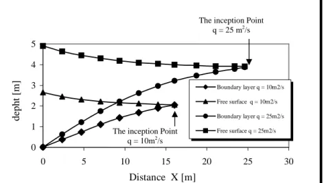
The inception point is then identified as the intersection of the computed outer edge of the boundary layer with the free surface (figure 2). We note that these curves have, indeed, a point of intersection and that this one moves downstream by increasing the discharge.
4.2 INFLUENCE OF DISCHARGE
Figure 3 illustrate the evolution of the boundary layer along the channel for various discharge, resulting from the application of the model to the stepped spillway M’Bali. One notices the increase, the thickness of boundary layer proportionally to the increase of the discharge. 4.3 PROFILES OF THE VARIABLES
The research of the effect of the step on the phenomenon of the natural ventilation of the flow constitutes the principal objective of our work. To arrive there, it was necessary to calculate at each point of the discretized field the values of the variables of the flow introduced into mathematical modelling
4.3.1 Velocity distribution
Figure 4 defers the profile of the velocity following the thickness of boundary layer to various sections for the discharge q = 20 m2 /s. One can separate the profiles of the velocity in two region : The first corresponds roughly to the interval :0< YYC <10 %. The second corresponds roughly to the interval : 10 %< YYC <100 %. In accordance with the development devoted to the decomposition of the boundary layer, the first region corresponds to the inner zone of the boundary layer where the molecular effect is dominating whereas the second corresponds to the external zone of the boundary layer where the wall-attachment effect tends to decrease as one approaches the limit of the free flow.
4.3.2 Turbulent kinetic energy and turbulent kinetic energy dissipation
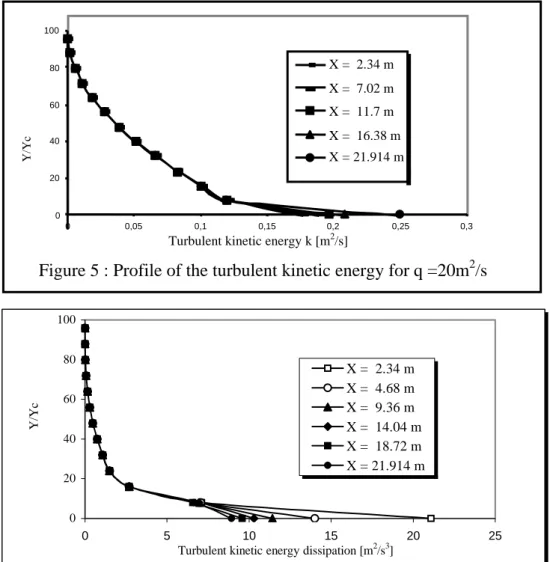
Figure 5 is shows the profile of the turbulent kinetic energy for the discharge q = 20 m2/s. Figure 6 presents the profile of the turbulent kinetic energy dissipation for the same discharge. The general paces of the profiles of the turbulent kinetic energy and the turbulent kinetic energy dissipation according to the thickness of boundary layer are similar but inversely proportional to the distribution speeds presented above. One records maximum values on the level of pseudo-bases from which, the paces decrease very quickly until certain heights of about 8 to 10 % of Y/Y C for turbulent energy and about 18 to 22 % of Y/Y C for the turbulent
energy dissipation. Thereafter, the variation becomes increasingly slow tending to cancel itself gradually while approaching the limit of the free flow. One observes that the turbulent kinetic energy increases from one section to another while going in the direction of the flow, whereas one records an opposite effect for the dissipation turbulent energy.
Figure 2 : Location of the start of air entrainment 0 1 2 3 4 5 0 5 10 15 20 25 30 Distance X [m] depht [m] Boundary layer q = 10m2/s Free surface q = 10m2/s Boundary layer q = 25m2/s Free surface q = 25m2/s
The inception Point q = 10m2/s
The inception Point q = 25 m2/s 2 q = 20m2/s q = 22 m2/s q = 24 m2/s q = 26m2/s q = 28 m2/s q = 32 m2/s q = 36 m2/s q = 40m2/s q = 46 m2/s q = 48 m2/s δ [m] 0,6 0,5 0,4 0,3 0,2 0,1 0 0 2 4 6 8 10 12 Length X
Figure 3 : Typical relationship between the boundary layer
thickness and distance
0 20 40 60 80 100 2 3 5 6 7 Velovity [m/s] Y/Yc X = 2.34 m X = 4.68 m X = 7.02 m X = 11.7 m X = 16.38 m X = 18.72 m X = 21.06 m
Figure 4 : Profiles of the velocity (q = 20 m2/s) 0 20 40 60 80 100 0 0,05 0,1 0,15 0,2 0,25 0,3
Turbulent kinetic energy k [m2/s]
Y/Yc X = 2.34 m X = 7.02 m X = 11.7 m X = 16.38 m X = 21.914 m
Figure 5 : Profile of the turbulent kinetic energy for q =20m2/s
0 20 40 60 80 100 0 5 10 15 20 25
Turbulent kinetic energy dissipation [m2/s3]
Y/Yc X = 2.34 m X = 4.68 m X = 9.36 m X = 14.04 m X = 18.72 m X = 21.914 m
Figure 6 : Profile of turbulent kinetic energy dissipation (q = 20 m2/s)
5. CONCLUSION
In this study, a numerical model is presented to analyse the location of the start of air entrainment by solving two dimensional equations. The turbulence stresses are closed by using k-ε model. We note that, the point of inception moves downstream by increasing the discharge. One notices the increase of the thickness of boundary layer proportionally to the increase of the discharge.
SYMBOLS d [m] Height of steps
dI [m] Flow depth at the inception point
f [ - ] Friction factor F* [ ] Froude number.
g [m/s2] Acceleration of gravity h [m] Flow depht
k Turbulent kinetic energy ks [m] Uniform roughness.
P [N/m2] Pressure.
q [m2/s] Discharge per unit width.
u, v [m/s] Velocity components in the x and y direction. Ul [m/s] Free stream velocity.
Uτ [m/s] Shear velocity
XI [m] Distance from the start of growth of boundary layer to the
inception point air entrainment
u’, v’ [m/s] Velocity fluctuation components in the x and y direction. α [°] Channel slope
δ [m] Boundary layer thickness
δinitial [m] Boundary layer thickness at the crest
κ - Von Karman constant µ Ns/m2 Dynamic viscosity µt Ns/m 2 Turbulent viscosity ν [m2/s] Kinematic viscosity ρ [Kg/m3] Fluid density τ0 [N/m 2
] Average bottom shear stress
ω Stream function
REFERENCES
[1] CHANSON, H. (1994). " Hydraulic Design of Stepped Cascades, Weirs and Spillways".
Pergamon, Oxford, UK, Jan., 292 pages.
[2] CHANSON, H. (1997). “Air Bubble Entrainment in Free-Surface Turbulent Shear Flows.” Academic Press, London, UK, 401pages.
[3] CHANSON, H., (2000). « Forum article. Hydraulics of Stepped Spillways: Current Status.” Journal of Hydr Engrg., ASCE, Vol. 126, No. 9 pp 636-637.
[4] HALBRONN, G. (1952). “Etude de la mise en Régime des Ecoulements sur les Ouvrages à Forte pente. Applications au problème d’Entraînement d’Air. » (‘Study of the Setting up of the Flow Regime on High Gradient Structure. Application to Air Entrainment Problem.’ Journal La Houille Blanche, N° 1, pp 21-40; N°3, pp 347-371; N°5, pp 702-722 (in French) [5] HALBRONN, G., DURAND, R. and COHEN de LARA, G., (1953)."Air Entrainment in Steeply Sloping Flumes." Proc. 5th IAHR Congress, IAHR-ASCE, Minneapolis, USA, pp. 455-466
[6] HANJALIC, K. and LAUNDER, B.E. (1972). "A Reynolds stress model of turbulence and its application to thin shears flows" Journal of fluid mechanics, vol. 52, part 4.
[7] HENDERSON, F.M., (1966)."Open channel flow". The MacMillan Compagny, New York, N.Y.
[8] HICKOX, G.H. (1945). “Air Entrainment in Spillway Flow.” Civil Engineering,, Vol. 15, No. 12, Dec., pp 562.
[9] HUANG, G., KAWAHARA, Y. and TAMAI, N. (1993). "Numerical investigation of buoyant shear flown with a multiple-time-scale turbulence model". Proceeding of the 5th international symposium, September, Paris, France.
[10] KIM, S.W. and CHEN, Y.S. (1988)."A finite element computation of turbulent boundary layer flows with an algebraic stress turbulence model" Comput. Math. Appl. Engin., Vol. 66. [11] KLEBENOFF, D.S. (1953). "Characteristics of turbulence in a boundary layer with zero pressure gradient". National Advisory Council for Aeronautics, T.N 3178.
[12] LANE, E.W. (1939). “Entrainment of Air in Swiftly Flowing Water. Observations of the flow over Spillways yield Conclusions of interest to Hydraulic Engineers.” Civil Engineering, No2, Feb.
[13] LAUNDER, B. E., and SPALDING, D. B., (1974). “The numerical computation of turbulent flows.” Computer methods in applied mechanics and engineering, vol. 3, pp. 269-289 [14] SCHLICHTING, K., (1968). "Boundary layer theory". Edition Mc. Graw-Hill.