Optimal Transport for Image Processing

(1)

HAL Id: tel-01246096

https://hal.archives-ouvertes.fr/tel-01246096v8

Submitted on 8 Nov 2017

HAL is a multi-disciplinary open access

archive for the deposit and dissemination of sci-entific research documents, whether they are pub-lished or not. The documents may come from teaching and research institutions in France or abroad, or from public or private research centers.

L’archive ouverte pluridisciplinaire HAL, est destinée au dépôt et à la diffusion de documents scientifiques de niveau recherche, publiés ou non, émanant des établissements d’enseignement et de recherche français ou étrangers, des laboratoires publics ou privés.

Optimal Transport for Image Processing

Nicolas Papadakis

To cite this version:

Nicolas Papadakis. Optimal Transport for Image Processing. Signal and Image Processing. Université de Bordeaux; Habilitation thesis, 2015. �tel-01246096v8�

(2)

HABILITATION À DIRIGER DES RECHERCHES

ÉCOLE DOCTORALE MATHÉMATIQUES

ET INFORMATIQUE

Spécialité: Mathématiques Appliquées

Transport Optimal pour le Traitement d’Images

présentée par

Nicolas Papadakis

Soutenue le 17 décembre 2015

devant le jury composé de:

M. Jean-François Aujol Professeur de l’Université de Bordeaux (Examinateur)

M. Jérémie Bigot Professeur de l’Université de Bordeaux (Examinateur)

M. Antonin Chambolle Directeur de Recherches CNRS (Rapporteur)

Me. Julie Delon Professeur de l’Université Paris Descartes (Examinateur)

M. Angelo Iollo Professeur de l’Université de Bordeaux (Examinateur)

Me. Étienne Mémin Directeur de Recherche Inria (Examinateur)

M. Patrick Pérez Directeur de Recherche Inria, Technicolor (Rapporteur)

(3)

Document préparé à

l’Institut de Mathématiques de Bordeaux (UMR 5251) 351 Cours de la Libération

(4)

(5)

(6)

Optimal Transport for Image Processing

Abstract

Optimal Transport is a well developed mathematical theory that defines robust metrics between probability distributions. The computation of optimal displacements between densities through the associated transport map makes this theory mainstream in several applicative fields. For image processing applications, the transport map can for instance be used to compute geodesics between images or to transfer characteristics of one image to another. In this con-text, it is of major interest to preserve the nature of the observed objects, in order to synthesize images that are physically and visually plausible. In this document, generalized Optimal Trans-port distances including relaxation and regularization are considered to improve the modeling of image processing problems. New models and algorithms within the continuous and discrete formulations of Optimal Transport are presented.

With the continuous setting, the integration of physical regularization of the transport plan makes possible the interpolation of ocean images containing complex structures.

In the discrete setting, the regularization of the transport plan is considered for color transfer between images. Convex and non-convex models are proposed to define automatic methods that adapt the proportion of colors required to synthesize visually plausible images. These methods are extended to the computation of barycenters to deal with the color normalization of multiple images.

Finally, the entropy regularization of discrete Optimal Transport is used for image segmenta-tion. A fast and convex model is designed to segment images, while respecting global color distribution constraints.

Keywords : Generalized Wasserstein distance, image processing, image interpolation, color transfer, segmentation, (non)convex optimization.

Résumé

Le Transport Optimal est une théorie mathématique très développée permettant de définir des métriques robustes entre distributions de probabilité. Le calcul du déplacement optimal entre densités par le plan de transport associé rend cette théorie attractive du point de vue applicatif. En traitement d’images, le plan de transport peut par exemple être utilisé pour calculer des géodésiques entre images ou encore transférer des caractéristiques d’une image vers une autre. Dans ce contexte, il est important de préserver le nature des objets observés afin de synthétiser des images physiquement et visuellement plausibles.

Dans ce document, des distances de Transport Optimal généralisées sont considérées pour améliorer la modélisation de problèmes de traitement d’images. De nouveaux modèles et algo-rithmes sont présentés pour les formulations continues et discrètes du Transport Optimal. Dans le cas continu, l’intégration de régularisation physique du plan de transport permet alors d’interpoler des images d’océan contenant des structures complexes.

Dans la formulation discrète, la régularisation du plan de transport est considérée pour le trans-fert de couleurs entre images. Des modèles convexes et non-convexes sont proposés pour définir des méthodes automatiques adaptant la proportion de couleur nécéssaire pour un transfert visuellement plausible. Ces méthodes sont également étendues aux barycentres afin d’aborder le problème de normalisation de couleurs entre plus de deux images.

La régularisation entropique du Transport Optimal discret est finalement utilisée pour la seg-mentation d’image. Un modèle convexe et rapide est proposé pour segmenter des images tout en respectant des contraintes globales sur les distributions de couleurs.

Mots-clefs : Distance de Wasserstein généralisée, interpolation d’images, transfert de couleur, segmentation, optimisation (non)convexe.

(7)

(8)

Chapter 1 Introduction

This habilitation manuscript presents a selected subset of the research activities realized in the period 2011-2015. It focuses on the use of Optimal Transport for image processing purposes. These works have been initiated through the supervision of two PhD thesis and one post-doctorate.

In this introduction, the applicative and scientific motivations of the realized works are presented. The main limitations of the use of Optimal Transport for Image Pro-cessing are then exposed. The related contributions are finally briefly presented, before detailing the organization of the document.

1.1 Motivations

Computer Vision Image and video contents are omnipresent in the world today,

both in our personal and professional lives. Technology is in constant evolution and the amount of data is everyday dramatically increasing. Market data indicates that the number of acquisition mobile devices is going to considerably increase. In particular, a spectacular growth in video users for the years to come is expected. In 2016, more than 1.6 billion electronic devices capable of recording and sharing pictures and videos will be used all around the world. Billions of raw images and videos are consequently diffused on the Internet. For instance, approximately 2 millions of pictures are uploaded on Flickr on a daily basis and the volume of videos uploaded to Youtube is gigantic, and constantly increasing (300 hours per minute). However, most of this video content is not exploitable because it has not been properly edited.

Due to the diversity of applications in which images are involved, the type of data is completely heterogeneous: color images, 3D images or even multidimensional images (including transparency, depth, etc), animated sequence and videos, multispectral im-ages, depth imim-ages, light-field, etc. Additionally, pictures are often captured at different resolutions and under different lighting conditions.

The need for generic methods to deal with this huge amount of data is increasing. The development of methods for a given application implies the control of the statistics of the images targeted by this application. An example is presented in Figure 1.1. Raw images diffused on the Internet are used for 3D reconstruction of buildings (using e.g.

(13)

12 _Motivations

geolocalized Flickr images) or virtual synthesis of 2D views of cities (Google street-view, Institut National de l’Information Géographique et Forestière, IGN). For these appli-cations, image harmonization is a key step to merge heterogeneous data with different color statistics. In order to circumvent this challenging task, the current methods only select a small subset of available images that are sufficiently close in terms of color and illuminations. As a consequence, most of existing data is not even used, whereas it could lead to significant improvements.

(a) (b)

Figure 1.1 – Example of massive use of images. (a) Reconstruction of the Colosseum from Flickr images [2]. (b) UrbanDive navigation system of IGN.

In order to use more images in this context or simply when one looks for pictures on the Internet to illustrate professional or personal presentations, the huge quantity of images needs to be efficiently indexed and retrieved. This requires very fast and efficient comparison tools between descriptors of image statistics, which are also of interest for object segmentation, editing or harmonization.

Histograms are popularly used in image processing, computer vision and machine learning to represent complex visual objects. To that end, relevant features such as color, contours, orientations or textures are first extracted from images. Histograms are built from the quantization of the space of features into discrete bins. One can further define normalized histograms that describe the frequencies of each of the observed features. The problems of retrieving a similar image in a database or segmenting a particular object can thus be recasted as a problem of histograms comparison. In this context, even if adapted metrics can be learned by neural networks for specific application, generic robust comparison tools are still needed for a broad use.

While a lot of research effort is dedicated to the enhancement of image descriptors (by adding additional information such as text or context) in a “big data” perspective, the common metrics used for statistics comparison are still not developed enough to deal with various perturbation effects (such as histogram quantization, shifts, deformation,

etc) or large amount of data outliers. Namely, spatial information is not efficiently

considered as it is mainly used to enhance the feature description [196]. Including spatial information into the distance defined on the feature space is an interesting alternative to improve the quality of the results.

The Optimal Transport framework is the proper way to compare statistic distribu-tions. In contrast to most distances from information theory, it takes into account the spatial location of the density modes [216]. By incorporating in its definition a ground metric between the features themselves, the Optimal Transport distance (that corre-sponds to the Wasserstein distance when the ground metric is the quadratic Euclidean distance) can compare sparse histograms even if their supports do not overlap

(14)

signif-CHAPTER 1. INTRODUCTION 13

icantly. Additionally, Optimal Transport provides a warping (the so-called transport plan) between histograms which can be used to perform image editing such as color transfer.

Optimal Transport framework has been shown to produce robust state of the art results for the comparison of statistical descriptors through the so-called Earth Mover’s Distance [187]. Various works on color image retrieval [162] or artistic image indexation [121] have shown on small datasets (i.e. thousands of images) that Optimal Transport framework is intrinsically designed to carry this spatial information. However, unless considering some crude approximations and/or simple ground metrics, it involves pro-hibitive computational costs. Though Optimal Transport would lead to a significant gap in performance improvement, this computational limitation is clearly an obstacle to its study and large scale deployment, when considering the dimension of image databases or the data itself (multi-spectral images, patch representation, tensor-field imaging, etc).

Geosciences Since the late seventies, many satellites have been launched to improve

our knowledge of the atmosphere and the oceans. Geostationary satellites provide, among other data, photographic images of the earth system. Sequences of such images show the dynamical evolution of identified meteorological or oceanic “objects”: fronts, clouds, eddies, vortices, etc. The human vision can easily detect the dynamics in this kind of image sequences and it clearly has a strong predictive potential. This aspect is favoured by the fact that image data, contrary to many other measurements, is dense in space and time. Indeed the spatial resolution of current METEOSAT satellites is close to one kilometer and they produce an image every 15 minutes. This frequency will be improved up to one every 10 minutes (and even every 2.5 minutes for Europe only) with the upcoming third satellite generation. It implies a huge quantity of information which can be seen as an asset but also induces difficulties for the assimilation system that has to cope with such amount of data.

Satellite data is currently used in operational systems for calibrating Numerical Weather Prediction models, mainly through the assimilation of the radiance measured by the satellite at each pixel of the image. As illustrated in Figure 1.2, satellite images are related to physical quantities such as surface temperature, sea surface height, cloud pressure, chlorophyll concentration, etc.

(a) (b) (c)

Figure 1.2 – Different examples of satellite images used for data assimilation. (a) Altimetric reconstruction from JASON satellite data. (b) Ocean color/ Chlorophyll from the MODIS captor of ENVISAT satellite. (c) Sea surface Temperature from the MODIS captor of ENVISAT satellite.

(15)

14 _Motivations

In practice only a tiny percentage (about 3 − 5%) of total satellite (from polar orbiting and geostationary) data is used in operational systems, while being given low confidence with respect to synoptic data, collected by stations, aircrafts, radiosounding, ballons or drifters. Considering the cost of satellite observing systems (the cost of the launch of the Meteosat Third Generation is estimated to about 2.5 billion Euros) and of the infrastructures required for the collection of the data itself, improving their impact on forecasting systems is an important topic of research.

As a consequence, there is a need to provide pertinent distances to interpolate be-tween the observed satellite images and the images of physical variables provided by the numerical models. The spatial information contained in satellite images is currently not

taken into account, as the classical “pixel-to pixel” L2 _{distance used in data assimilation}

is not adapted to deal with bad localization of structures such as clouds, vortex or fronts [209], [52]. If the same structure is contained in both images at different locations, an

interpolation should deal with the spatial shift. While a L2 _{interpolation would create}

two structures, Optimal Transport is intrinsically designed to correctly interpolate the position of the structure along the geodesic in the Wasserstein space.

Considering images as densities, interpolation between images can be realized with the Optimal Transport map [112]. It is thus an interesting framework in order to pro-pose new metrics for data assimilation [159]. In this context, an important challenge is to model the topology of the considered domain (coasts or islands in oceanography) for estimating image interpolations that have a real physical meaning. In this context, even if Optical Flow methods can be considered for data assimilation to compute dis-crepancies between atmospheric images [68], they can not deal with complex domains in oceanography [27].

Optimal Transport Optimal Transport is a well developed mathematical theory that

defines a family of metrics between probability distributions [105, 216]. These metrics measure the amplitude of an optimal displacement according to a so-called ground cost defined on the space supporting the distributions. The resulting distance is referred to

as the Wasserstein distance in the case of Lp ground costs C(x, y) = ||x−y||p. As shown

in Figure 1.3, it measures the minimal effort required for filling a “remblai” (−µ1) with

a “déblai” (µ0), i.e. transporting one distribution to another. The geometric nature of

Optimal Transport, as well as the ability to compute optimal displacements between densities through the corresponding transport map T , make this theory progressively mainstream in several applicative fields.

Figure 1.3 – Illustration of Optimal Transport between distributions µ0 and µ1 as

introduced in [145] with the “déblais” and “remblais” problem . Interpolations (µt)t∈[0;1]

(16)

CHAPTER 1. INTRODUCTION 15

Early successes of applications of Optimal Transport were mostly theoretical, such as the study of shape recognition [106], the derivation of functional inequalities [67], the construction of solutions of non-linear partial differential equations [124] or the study of gradient flows in Wasserstein spaces [5].

In computer vision, the Wasserstein distance has been shown to outperform other metrics between distributions for machine learning tasks [187, 163, 75] or image segmen-tation [151, 165, 206].

In image processing, the warping provided by the Optimal Transport has been used for video restoration [82], color transfer [168], texture synthesis [95], optical nanoscopy [45] and medical imaging registration [112]. It has also been applied to interpolation in computer graphics [35, 199] and surface reconstruction in computational geometry [85]. Optimal Transport is either used to model various physical phenomena, such as for instance in astrophysics [101] and oceanography [17, 97].

1.2 Limitations of Optimal Transport in Imaging

The numerical resolution of the Optimal Transport problem raises several challenges. This is the main reason why it has been poorly used in image processing until re-cently. Computing Optimal Transport distance is only an easy task when dealing with one-dimensional densities, such as histograms of grayscale images, or multi-dimensional densities roughly discretized. However, when considering transport between images themselves or when dealing with statistics of color images, the densities are defined on higher dimensional spaces. Hence, the versatility and high quality of Optimal Transport distances come at a price for general image applications: they require the resolution of high dimensional problems that scale with the product of the dimensions of the dis-cretized densities.

In this context, the fluid dynamic formulation of the Optimal Transport problem introduced in [19] is an interesting approach for dealing with higher dimensions. The entropic regularization proposed in [73] has also offered new perspectives as faster algo-rithms based on Sinkhorn distances can be designed for computing approximate Optimal Transport in larger dimensions. This last approach gives interesting approximations of the transport distance but leads to transport maps that may be too far from the optimal ones for transfer and interpolation purposes.

Hence, generalizations of the Optimal Transport distances are still necessary to adapt to applications involving image processing. For instance, when the transport plan is used to interpolate between densities that have very different “shapes” or contain data outliers, partial models able to relax the constraint of transporting the whole mass are required. In this context, another flaw for the use of Optimal Transport plan is that it is usually highly irregular. For the interpolation between images or histograms of features, dedicated regularizations of the transport plan are needed to preserve either the nature of the objects contained in the images or the modes of the statistics.

Such property is illustrated in Figure 1.4 with an example of color transfer between images. If the exact prescription of color is realized with the Optimal Transport map, visual artifacts may appear.

(17)

16 _{Contributions and Organization of the document}

Figure 1.4 – Illustration of the limitation of Optimal Transport for color transfer. The

Optimal Transport map T between the color distributions of the middle parrot µ0 and

the left parrot µ1 is computed. The map is then used to modify the colors of the middle

parrot in order to obtain the right one. As the transport map is highly irregular, very different colors are assigned to pixels of the background that were originally close both in spatial and color spaces.

Finally, introducing Optimal Transport distances in more general image problems such as segmentation, involving histogram data fitting and spatial regularization in the image domain, is even more challenging. Spatial regularization can be incorporated through graph or variational modeling. However, graph based approaches are limited to simple bin-to-bin metrics between histograms [185] and cannot deal with Optimal Transport distances without leading to problems of gigantic size [200]. Slow hybrid methods that alternate optimization on graph and Optimal Transport computation should be designed. Variational methods may thus be more adapted to such problems, since the computation of Optimal Transport distances can be integrated into a general model that can directly be optimized.

1.3 Contributions and Organization of the document

In this document, some new variational image processing models using Optimal Trans-port distances are exposed. The main common contribution of the presented works is to propose original modeling of classical problems such as image interpolation, color transfer or image segmentation, while considering recent optimization methods able to solve these problems with “reasonable” computational cost (several seconds to several minutes).

For that purpose, extended Optimal Transport models including relaxation of the mass constraint and regularization of the transport map are introduced. These gener-alized Optimal Transport models have been designed in both continuous and discrete settings. The continuous formulation is applied to image interpolation, while the discrete one is used for color transfer and image segmentation.

(18)

CHAPTER 1. INTRODUCTION 17

The problems associated to both formulations of Optimal Transport are illustrated in Figure 1.5. In the continuous framework, the images are considered as continuous

densities µ0 and µ1 defined on a domain Ω. The transport map is in this case a vector

field, defined from Ω to Ω, that transfers µ0 onto µ1. The problem can be expressed in a

dynamic way through a fluid mechanics formulation. In the discrete setting, normalized histograms of features extracted from images are considered. When computing the static transport between histograms X and Y discretized with M and N bins, an acceptable transport map is a M × N matrix describing a joint distribution P which marginals

are the given histograms (i.e. PjPi,j = Xi and PiPi,j = Yj). Hence Pi,j is the mass

transferred from Xi to Yj.

(a) Continuous transport (b) Discrete transport matrix P

velocity field T : Ω → Ω coupling histograms X and Y

Figure 1.5 – Illustration of the transport map in the (a) continuous and (b) discrete

formulations of the Optimal Transport problem. In (b), white color represents Pi,j = 0.

Overview of the manuscript The first part of this document is dedicated to some

contributions in the continuous setting. Chapter 2 is based on [160] and presents an ap-proach for the numerical estimation of the geodesic path between two densities according

to the L2 _{Wasserstein metric. Generalizations including additional physical constraints}

proposed during the PhD of R. Hug in [120] for application to the interpolation of ocean images are next presented in Chapter 3.

The second part focuses on contributions in the discrete setting. Chapter 4 presents the relaxed and regularized formalism proposed in [93] as well as entropic regularization recently introduced in the literature [73]. Chapters 5 and 6 are respectively dedicated to the application of these tools to color transfer between images and image segmentation. Chapter 5 gathers methods initiated during the Postdoctorate of S. Ferrandans [94, 178], while Chapter 6 reviews some models introduced during the PhD of R. Yıldızoğlu [221, 222, 176].

In order to make the manuscript self-content, standard first-order proximal algo-rithms dedicated to the optimization of non-smooth functionals used all along the doc-ument are finally presented in Appendix A.

(19)

(20)

Part I

Continuous Optimal Transport

(21)

(22)

Chapter 2 Dynamic Optimal Transport

This chapter is focused on the computation of geodesics for the Optimal Transport

metric associated to the L2 _{ground cost. It reviews various methods and extends the}

approach pioneered in [19] from the perspective of proximal operator splitting in convex optimization [160]. It shows the simplicity and efficiency of this method, which can easily be extended beyond the setting of Optimal Transport by considering various convex cost functions that will be presented in Chapter 3.

2.1 Estimation of the Transport Map

Let Ω be a convex and bounded domain of Rd_{and ρ}

0, ρ1be two non-negative L1functions

on Ω, of equal mass. We will assume without loss of generality that Z Ω ρ0(x) dx = Z Ω ρ1(x) dx = 1. (2.1)

The original formulation of the Optimal Transport problem in [145] corresponds to

minimizing the cost for transporting a ρ0 onto ρ1 using a map T . In the following, we

restrict our exposition to maps T : Ω ⊂ Rd _{7→ Ω}_{. A valid transport map T : Ω → Ω}

then pushes forward the measure ρ0(x)dx onto ρ1(x) dx, that is T #ρ0 = ρ1 or for all

bounded set A ⊂ Ω: Z A ρ1(x)dx = Z T (x)∈A ρ0(x)dx. (2.2)

In term of densities, when T is smooth and one-to-one, the constraint T #ρ0 = ρ1

corresponds to

ρ0(x) = ρ1(T (x)) |det(∇T (x))| (2.3)

where ∇T (x) ∈ Rd×d _{is the differential of T at x. This is known as the Jacobian}

equation. We call T (ρ0, ρ1) the set of transport maps that satisfy the constraint (2.3).

The Lp _{Kantorovitch-Wassertein distance between ρ}

0 and ρ1 is then defined by

Wp(ρ0, ρ1)p = inf

T ∈T (ρ0,ρ1)

Z

|T (x) − x|pρ0(x)dx.

(23)

22 _{Estimation of the Transport Map}

The Lp _{Monge-Kantorovitch problem corresponds to finding a mapping T such that}

this infimum is achieved. It can be recasted as

Wp(ρ0, ρ1)p = min

T ∈T (ρ0,ρ1)

Z

C(x, T (x))ρ0(x) dx (2.4)

where C(x0, x1) ≥ 0is the ground cost of transporting x0 ∈ Ω onto x1 ∈ Ω.

Let us now detail how estimating the transport map T with Partial Differential Equations.

Optimal Transport and PDEs The Optimal Transport for the L2 _{ground cost has}

a special structure. It can be shown to be uniquely defined (see e.g. [216] page 66) and the transport map is the gradient of a convex potential Ψ from Ω to R:

T (x) = ∇Ψ(x). (2.5)

Hence, one can show that the mass transfer associated to a L2 ground cost follows

straight lines [41], which can be used for developing specific Lagrangian solvers [122]. Other class of methods relies on the fact that from relations (2.3) and (2.5), the convex function Ψ is solution of the Monge-Ampère equation:

det(D2Ψ)ρ1(∇Ψ(x)) = ρ0(x).

This equation being highly nonlinear, numerical methods to solve the Monge-Kantorovitch problem based on discretization of the Monge-Ampère equation have been investigated [157, 135, 79, 154, 23, 24]. A major difficulty in these approaches is to deal with compactly supported densities, which requires a careful handing of the boundary conditions [102].

Another line of methods iteratively constructs mass preserving mappings converging to the Optimal Transport [6, 111, 38]. This explicitly constructs the so-called polar factorization of the initial map, see also [18] for a different approach. These PDE’s based approaches to the resolution of the Optimal Transport have found several applications, such as image registration [112], density regularization [46], optical flow [63] and grid generation [204].

A last axis of research consists in using gradient flows where the gradient direction is computed according to the Wasserstein distance. This was initially proposed in [124] to build solutions to certain non-linear PDE’s. This technique is now being used to design numerical approximation schemes for the solution of these equations, see for instance [51, 89, 96, 22].

All these approaches are nevertheless limited to positive densities, or to non-negative

densities with a convex support of the target density ρ1, which is a real limitation for

image processing applications. The only numerical method that can deal with

non-negative datahas been proposed by Y. Brenier et J.D. Benamou through a Fluid

(24)

CHAPTER 2. DYNAMIC OPTIMAL TRANSPORT 23

2.2 Fluid Mechanics Formulation

Instead of computing directly the transport, it is possible to consider the geodesic path between the two densities according to the Wasserstein metric (the so-called

displace-ment interpolation [142]). For the L2 _{ground cost, the geodesic path between the}

mea-sures with densities ρ0 and ρ1 can be shown to have density t 7→ ρ(t, x) where the

additional dimension t ∈ [0, 1] parameterizes the path interpolating linearly between

the identity map Idd and the Optimal Transport map T :

ρ0(x) = ρ(t, Tt(x)) |det(∇Tt(x))| where Tt= (1 − t) Idd+tT.

The geodesic can thus be computed by first obtaining the transport and then making the densities evolve. In [19], it has been demonstrated that this geodesic solves the

following non-convex problem over the densities ρ(t, x) ∈ R+and a velocity field v(t, x) ∈

Rd checking the continuity equation.

Theorem 1 (Benamou-Brenier). In case p = 2 the Wasserstein distance between ρ0

and ρ1 is such that:

W (ρ0, ρ1) = inf ρ,v Z Ω Z 1 0 ρ(t, x)|v(t, x)|2dxdt (2.6)

the infimum being taken on ρ, v verifying the non-linear constraint

C0 = {(ρ, v), ∂tρ + divx(ρv) = 0, hv, ~ni = 0, ρ(0, ·) = ρ0, ρ(1, ·) = ρ1}, (2.7)

with homogeneous Neumann conditions on the velocity field v, through ~n which is the

normal of the domain Ω.

While the estimation of the L2 Wasserstein distance (2.4) is a static problem over Ω,

the introduction of the additional dimension t and the velocity field v leads to a dynamic problem involving kinetic energy (2.6) and continuity equation (2.7) on Ω × [0; 1].

2.3 Convexification

Following [19] and introducing the change of variable (ρ, v) 7→ (ρ, m), where m is the momentum m = ρv, we obtain a convex optimization problem over the couple (ρ, m):

min (ρ,m)∈CJ (ρ, m) := Z 1 0 Z Ω J (ρ, m)dxdt (2.8)

which deals the positivity constraint [49]: J (ρ, m) =    ||m||2 2ρ if ρ > 0 0 if (ρ, m) = (0, 0) +∞ otherwise. (2.9) The set of constraint C becomes linear and reads:

(25)

24 _{Discretization and Optimization}

Denoting as ιC(x) = 0 if x ∈ C, +∞ otherwise, the convex problem introduced in

[19] reads:

(ρ∗, m∗) = argmin

ρ,m

J (ρ, m) + ιC(ρ, m). (2.11)

Notice that with this formulation, we are not able to compute the transport map and we only estimate the geodesic ρ(x, t). The existence of minimizers of such a problem

in the space of measures has been studied in [217]. The existence of L2 _minimizers

for positive data (ρ0, ρ1) has been studied in [110]. The existence of L2 minimizers for

nonnegative data (ρ0, ρ1)has been shown during the PhD of Romain Hug [119], in which

the uniqueness of the variable ρ has also been established.

As the problem (2.11) is convex and non-smooth, the Alternating Direction Method of Multipliers (ADMM, see (A.9)) algorithm was considered in [19] to compute a global minimizer. Nevertheless, other proximal method that are introduced in Appendix A can be used to compute a global minimizer.

2.4 Discretization and Optimization

In order to solve problem (2.11) over the sptaial domain of the image denoted as Ω, the dimension has to be increased with T time steps of artificial time t. The dimension of the variable ρ to estimate is therefore of size |Ω|T .

In [160], it has been proposed to rely on a staggered grid for the discretization of the continuity equation (2.10), similarly to the discretization of PDE’s in incompressible fluid dynamics (see for instance [113]). An interpolation operator I has then been considered for computing the cost function (2.9) on the regular grid. The use of a staggered grid is very natural in the context of the discretization of a divergence operator

associated to a vector field on Rd_.

The basic idea is to perform an accurate evaluation of every partial derivative at prescribed nodes of a cartesian grid using standard centered finite differences. Hence, the discrete problem (2.11) can be reformulated as:

(ρ∗, m∗) = argmin

(ρ,m)∈Es

J (I(ρ, m)) + ιC(ρ, m), (2.12)

The problem (2.12) consists in minimizing the sum of two non-smooth convex func-tionals, the first one being composed with a linear operator I. We can thus make use of proximal splitting methods such as Douglas Rachford (A.6) or Primal Dual (A.15) algorithms to solve this problem. As illustrated in the Figure 2.2, faster convergence was observed considering these algorithms instead of the ADMM one. To apply such algorithms that are described in the Appendix, the fundamental point is to be able to

compute the proximal operators (defined in relation A.2) of functions J and ιC.

Since the functional J is separable, the proximal operator of J can be computed

independently as the proximal operator of J for each point (˜ρ, ˜m)(t, x) ∈ R × Rd with

(t, x) ∈ [0; 1] × Ω. As shown in [160], it simply requires to solve a third order polynomial

(26)

CHAPTER 2. DYNAMIC OPTIMAL TRANSPORT 25

Finally, the proximal mapping of ιC is ProjC the orthogonal projector on the convex

set C. It requires solving a Poisson equation on the centered grid with prescribed boundary conditions. It can be achieved with Fast Fourier Transform in O(NP log(NP )) operations where N and P are number of spatial and temporal points, see [201].

Using this method, one can estimate the geodesic path between densities that van-ishes on the spatial domain, as illustrated in Figure 2.1.

t = 0 t = 1/4 t = 1/2 t = 3/4 t = 1

Figure 2.1 – Transport between characteristic functions. Evolution of ρ?_{(·, t)}_{for several}

values of t. The red curve denotes the boundary of the area with positive density.

2.5 Limitations and Motivations

A first limitation of this approach concerns the computational time. As exhibited in Figure 2.2, as the problem is not strictly convex, the convergence of the cost function

J is fast but the convergence of the iterates (ρk_{, m}k₎ _{is much slower.}

(a) J (ρk_{, m}k₎ _{(b) ||ρ}k_{− ρ}∗_||2

Figure 2.2 – Illustration of the convergence of the minimization process. (a) The cost function J reaches its minimum with a thousand iterations. (b) The convergence of

the iterates ρk to ρ∗ _{is slower. The reference solution ρ}∗ _{has been previously obtained}

with 108 _{iterations. Different proximal algorithms (ADMM, symmetric and asymmetric}

(27)

26 _{Limitations and Motivations}

Numerical instabilities may also happen when input data are not smooth enough, as illustrated by Figure 2.3. This is nevertheless not a issue for the targeted application where data are images of the ocean representing continuous fluids.

ρ0 ρ(1/6) ρ(1/3) ρ(1/2) ρ(2/3) ρ(5/6) ρ1

Figure 2.3 – Image interpolation between Gaspard Monge (ρ0) and Leonid Kantorovitch

(ρ1). Numerical instabilities appear (mainly on the boundaries of the head) since the

data are not smooth enough.

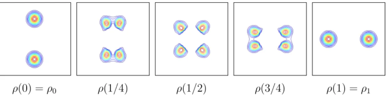
Next, when solving the Optimal Transport problem between two densities, we know that the mass transfer will follow straight lines. The structures contained in the original data can thus disappear along the optimal path. Such behavior is illustrated in Figure 2.4 that presents the optimal path between images containing two Gaussians.

ρ(0) = ρ0 ρ(1/4) ρ(1/2) ρ(3/4) ρ(1) = ρ1

Figure 2.4 – Two Gaussians examples. The Gaussians, represnted by their level lines,

split along the optimal path between ρ0 and ρ1.

One main objective for image interpolation is to incorporate some physical priors in order to preserve the structures contained in the data along the optimal path. This will be of main interest for geoscience imaging applications. Ocean and atmosphere, observed with satellites, are indeed driven by complex physical laws. The temporal interpolation of such satellite images is an important problem in this community and it should correspond to the underlying dynamics. As interpolation with Optimal Transport involves constant mass transport along straight lines, it is not a satisfactory solution.

In order to be able to process oceanographic images that contains “obstacles” such that continent or islands, the topology of the considered spatial model should be carefully taken into account.

(28)

Chapter 3 Generalizations for Image

Interpolation

In this Chapter, we consider generalized distances based on convex ground costs within the dynamical Optimal Transport formulation. In the aim of interpolating satellite images of the ocean in the presence of coasts, the computation of Optimal Transport on Riemannian manifolds modeling the spatial domain is tackled. Physical regularizations of the transport map are also considered. The numerical scheme proposed in the Chapter

2 can be used with only slight modifications with respect to the L2_{-Wasserstein case.}

3.1 Generalized Cost Functions

The formulation of the geodesic computation as a convex optimization problem pre-sented in Chapter 2 enables the definition of various metrics obtained by changing the objective function. Transport with congested dynamics [48] or unbalanced transport between densities that have different mass [136, 60] are namely possible. One can also

interpolate between different distances. An interpolation between the L2_-Wasserstein

and L2 _{distances is proposed in [20]. Lastly, an interpolation between L}2_-Wasserstein

and H−1 _{distances is described in [86]. This extension relies in a crucial manner on}

the convexity of the extended objective function, which enables a theoretical analysis to characterize minimizing geodesics [49].

Optimal Transport on Riemannian manifolds Many properties of the L2

-Was-serstein distance can be extended to the setting where the ground cost is the square of the geodesic distance on a Riemannian manifold. This includes in particular the existence and uniqueness of the transport map [141]. Displacement interpolation for transport on manifolds has the same variational characterization as the one introduced in [20] for Euclidean transport, see [217] for a detailed review of Optimal Transport on manifolds.

Displacement interpolation between two measures, each one composed of a single Dirac, amounts to computing a single geodesic curve on the manifold. Discretization and numerical solutions to this problem are numerous. A popular method is the Fast Marching algorithm introduced jointly by [195, 211] for isotropic Riemannian metrics

(29)

28 _{Generalized Cost Functions}

(i.e. when the metric at each point is a scalar multiple of the identity) discretized on a rectangular grid. This algorithm has been extended to compute geodesics on 2-D triangular meshes with only acute angles [128]. More general discretizations require the use of slower iterative schemes, see for instance [36].

Interpolation between pairs of measures in Riemannian manifolds generalizes to barycenters of a family of measures, see [127]. The numerical computation of Optimal Transport on manifolds has been less studied. For weighted sums of Diracs, displace-ment interpolation is achieved by solving a linear program to compute the coupling between the Diracs and then advancing the Diracs with the corresponding weights and constant velocity along the geodesics.

Hence, we have proposed in [160] to extend the method of [20] to solve for the displacement interpolation on a Riemannian manifold. Following [86, 49], we use a generalized cost function that allows one to compute geodesics that interpolate between

the L2_{-Wasserstein and the H}−1 _{geodesics . To introduce further flexibility, we have}

also considered a spatially varying tensor [120], which corresponds to approximating a transportation problem on a Riemannian manifold.

To that end, the convex cost functional (2.9) is generalized, for β ∈ [0; 1] and A(t, x) a symmetric positive definite tensor, as

J_βA(ρ, m) =    kAmk2 2ρβ if f > 0, 0 if (m, ρ) = (0, 0), +∞ otherwise. (3.1) and we now consider the problem:

(ρ∗, m∗) = argmin ρ,m Z 1 0 Z Ω J_βA(ρ, m) dx d t + ιC(ρ, m). (3.2)

The matrix A(t, x) is of size d × d and represents the anisotropic penalization of the

displacement energy. The isotropic case of constant weights A = Iddis studied in [86, 49].

The case β = 1 corresponds to the Wasserstein L2 _{distance. In a continuous (not}

discretized) domain, the value of the problem (3.2) for β = 0 is equal to the H−1 _Sobolev

norm over densities kρ0− ρ1k_H−1, as detailed in [86]. In this case, the induced distance

is an Hilbertian norm, and the corresponding geodesic is a linear interpolation of the

input measures. Thus, for measures having densities, one obtains ρt= (1 − t)ρ0+ tρ1.

3.1.1 Interpolation between L

2

-Wasserstein and H

−1

With this previous formulation (3.1), it is possible to interpolate between L2-Wasserstein

and H−1 _{geodesics. This is illustrated in Figure 3.1, which presents the level-lines of the}

estimated densities ρ(t, ·) for A = Iddand different values of β. It shows the evolution of

the solution between a linear interpolation of the densities (β = 0) and a displacement interpolation with transport (β = 1).

With this β parameter, smoother interpolation are then obtained. As illustrated in Figure 3.2, it is of interest for interpolating between non-smooth images and avoid numerical instabilities.

(30)

3.1.2 - Modelling of obstacle 29 β = 0 β = 1 / 4 β = 1 / 2 β = 3 / 4 β = 1 t = 0 t = 1/8 t = 1/4 t = 3/8 t = 1/2 t = 5/8 t = 3/4 t = 7/8 t = 1

Figure 3.1 – Display of the level sets of ρ(t, ·) for several value of t and β. For t = 0

and t = 1, ρ(t, ·) exactly corresponds to ρ0 and ρ1.

β = 1 β = 3 / 4 ρ0 ρ(1/6) ρ(1/3) ρ(1/2) ρ(2/3) ρ(5/6) ρ1

Figure 3.2 – Interpolation between Gaspard Monge (ρ0) and Leonid Kantorovitch (ρ1).

The first line is the same as in Figure 2.3. On the second line, by taking β = 0.75, a smoother interpolation between images is estimated.

3.1.2 Modelling of obstacle

When β = 1 and the matrices A(t, x) = Iddw(x) are diagonal and constant in time,

the solution of (2.12) discretizes the displacement interpolation between the densities

(ρ0, ρ1)for a ground cost being the squared geodesic distance on a Riemannian manifold.

We exemplify this setting by considering Optimal Transport with obstacles, which

corresponds to choosing weights w that are infinity on the obstacle O ⊂ R × Rd_{, i.e.}

(31)

30 _{Generalized Cost Functions}

Note that with such definition, the obstacles can be dynamic, i.e. the weight w does not need to be constant in time. Figure 3.3 shows a first example where O is a 2-D (d = 2) static labyrinth map (the walls of the labyrinth being the obstacles are displayed

in black). We use a 50 × 50 × 100 discretization grid of the space-time domain [0, 1]3

and the input measures (ρ0, ρ1) are Gaussians with standard deviations equal to 0.04.

For Gaussians with such a small variance, this example shows that the displacement interpolation is located closely to the geodesic path between the centers of the gaussians.

t = 0 t = 1/9 t = 2/9 t = 1/3 t = 4/9

t = 5/9 t = 2/3 t = 7/9 t = 8/9 t = 1

Figure 3.3 – Evolution of ρ(t, ·) for several values of t, using a Riemannian manifold with weights w(x) (constant in time) restricting the densities to lie within a 2-D static labyrinth map.

Isotropic Riemannian metrics corresponds to matrices A(t, x) = w(x) Idd

propor-tional to the identity at each point, but this extends to arbitrary Riemannian metrics

A(t, x) = A(x). The existence of a solution of the Monge-Kantorovitch problem on

Rie-mannian manifolds has been shown in [141]. The equivalence with a fluid mechanism formulation has been studied in [120]. In the case of a time dependent tensor A(t, x), even if the numerical algorithms are still providing a seemingly sound solution (see Fig-ure 3.4), there are no equivalence with any static Optimal Transport problem and the proof of existence of solutions remains an open subject.

Figure 3.4 shows a more complicated setting that includes a labyrinth with moving walls: a green wall appears at time t = 1/4 and a red one disappears at time 1/2. The difference with respect to the previous example is the fact that w is now time dependent. This simple modification has a strong impact on the displacement interpolation. Indeed, the speed of propagation of the mean of the density is not constant anymore since the density measure is confined in a small area surrounded by the walls for t ∈ [1/4, 1/2].

3.1.3 Anisotropic transport

The introduction of the anisotropy modeling through non diagonal matrices A is now illustrated. With adequate matrices A, it is now possible to define a polarization of

(32)

3.1.3 - Anisotropic transport 31

t = 0 t = 1/9 t = 2/9 t = 1/3 t = 4/9

t = 5/9 t = 2/3 t = 7/9 t = 8/9 t = 1

Figure 3.4 – Evolution of ρ(t, ·) for several values of t, using a Riemannian manifold with weights w(t, x) (evolving in time) restricting the densities to lie within a 2-D dynamic labyrinth map (i.e. with moving walls in green and red).

the space for modeling anisotropic domain priors. This problem is illustrated in Figure 3.5, which presents the optimal path between a horizontal and a vertical line on a square image. For these experiments, we defined different complex anisotropies, that are represented with the arrows of the first image of each line. If prior knowledge is available on the data, one can build a specific Riemannian manifold and the anisotropic model will therefore be able to simulate rigid or divergence free transports. This modelling is nevertheless not sufficient for more general purposes and we now propose to directly include physical prior into the model and not into the domain.

ρ0 ρ∗(1/8) ρ∗(1/4) ρ∗(3/8) ρ∗(1/2) ρ∗(5/8) ρ∗(3/4) ρ∗(7/8) ρ1

Figure 3.5 – Illustration of the mass ρ∗_(t) _{estimated between ρ}

0 and ρ1, through the

computation of the transport costs defined by two different anisotropic domains Ak,

illustrated by the blue directions in the first column of the two last rows. The first row is the isotropic transport.

(33)

32 _{Optimal Transport with physical priors}

3.2 Optimal Transport with physical priors

With the previous formulation, it is now possible to deal with islands for processing ocean images. Our underlying objective is to incorporate physic priors into the Optimal Transport model. More precisely, for general images, we would like to consider incom-pressible or rigid transports. Such transports can indeed prevent the object contained within the data from splitting along the computed paths, as for classical transport of Figure 2.4. The physical constraints can be characterized using the velocity, that is not a variable of the problem (2.11) anymore and should be reintroduced. We thus come

back to the classic Optimal Transport framework with β = 1 and A = Idd.

3.2.1 Non-convex coupling

In order to have a coupling between the variables (ρ, m) and v, a natural idea is to

consider the term ιD(ρ, m, v) = 0, with the set D = {m = ρv}. As D is not convex and

ιD non-smooth, we rather consider a differentiable coupling1:

K(ρ, m, v) = 1 2 Z Ω Z 1 0 ||m − ρv||2dx d t.

In [120], specific kind of transports were promoted regarding velocity priors that depend on the targeted application, as can be done with physical regularization of Optical Flow for fluid image sequences [69, 223]. A new functional term R(v) is thus introduced. This term can be defined as:

• Divergence-free: R(v) = ιCv(v), Cv = {div_xv(t, ·) = 0, hv(t, ·), ~ni = 0, ∀ t ∈ [0; 1]}, • Incompressible penalization: R(v) = R1 0 || divx(v(t, ·))|| 2 L2_(Ω)d t, • Rigid penalization: R(v) = R1 0 ||(∇xv(t, ·) + (∇xv(t, ·)) T_)/2||2 L2_(Ω)d t, • Translation penalization: R(v) = R1 0 ||(∇xv(t, ·)|| 2 L2_(Ω)d t.

By translation penalization, we mean a penalization of the deviation of a velocity field from translations. These terms are convex and the three last ones are differentiable. The existence of minimizers for the translation case has been shown in [120]. The generalized Optimal Transport model we are interested in now reads:

min

ρ,m,vF (ρ, m, v) := J (I(ρ, m)) + ιC(ρ, m) + λK(I(ρ, m), I(v)) + αR(v) (3.3)

where λ, α ≥ 0 respectively weight the coupling between variables and the velocity regularization term. The problem (3.3) is not convex in (ρ, m, v) but it is separately convex in (ρ, m) and in v. As the coupling is differentiable and the non-smooth terms are separable, following [210], we can perform a block coordinate descent with Algorithm (A.19) and minimize alternatively each convex problem in (ρ, m) and in v to obtain a critical point of the joint problem (3.3). Each subproblem can be solved with Algorithms presented in Appendix A.

1_{In [139], a different choice has been made and the problem is solved on (ρ, v) while penalizing the}

(34)

3.2.2 - Synthetic tests 33

3.2.2 Synthetic tests

First of all, we compare in Figure 3.6 the results obtained with the incompressible, translation and rigid penalizations on the two Gaussians example. Contrary to standard transport shown in Figure 2.4, such physical priors prevent the mass from splitting along the computed path. The Gaussians are deformed with the divergence-free prior, but it can be seen that the length of the level lines of the densities are preserved along the path. It is also important to underline that both translation and rigid penalizations keep the exact shapes of the two Gaussians along time. One can see in Figure 3.7 representing both computed paths, that the rigid penalization really performs a rotation and not a translation, so that the optimal path is no more composed of straight lines.

Div

ergence free

Translation

Rigid

ρ(0) = ρ0 ρ(1/4) ρ(1/2) ρ(3/4) ρ(1) = ρ1

Figure 3.6 – Two Gaussians experiments with penalization and a null initialization. Plot of the isolevels of the density ρ(t) along the different computed optimal path. The top line is realized with incompressibility (i.e. divergence free) penalization, the second with a translation penalization and the last one with a rigid penalization.

Translation penalization Rigid penalization

Figure 3.7 – Two Gaussians experiment. Plot of the whole trajectory computed with the translation and the rigid penalization models. The rigidity here involves a rotation.

(35)

34 _{Optimal Transport with physical priors}

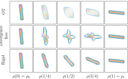
In the example of Figure 3.8 that presents a rotating bar, the rigid penalization (last line) recovers a quasi-rotation, which better preserves the prior physics with respect to pure Optimal Transport (first line). As expected, it can also be observed in Figure 3.9 that the length of the level lines of the estimated density are preserved with the incompressible and rigid penalization approaches. We refer the reader to [39, 120] for more synthetic examples involving such penalizations.

OT

Div

ergence free

Rigid

ρ(0) = ρ0 ρ(1/4) ρ(1/2) ρ(3/4) ρ(1) = ρ1

Figure 3.8 – Bar experiment. Plot of the isolevels of the density ρ(t) along the optimal path computed with different approaches. The first line is the Optimal Transport, the second is the proposed approach with an incompressible penalization and the last one with a rigid penalization that conserves the nature of the object to transport.

Optimal Transport Incompressible penalization Rigid penalization

Figure 3.9 – Bar experiment. Evolution of the length of the upper level lines of the estimated density along time t: |ρ(t, x) > i/10|, for i = 1 . . . 9 . The left plot is the classic Optimal Transport, the middle one corresponds to the incompressible penalization and the right one corresponds to a rigid penalization. Penalizing the norm of the velocity makes the level lines almost preserved along the computed path.

(36)

3.2.3 - Image interpolation in oceanography 35

3.2.3 Image interpolation in oceanography

In order to study the state of the oceans, snapshot images are produced by opera-tional numerical codes such as the Ocean Circulation Model NEMO (http://www.nemo-ocean.eu/) . The synthesis process is nevertheless time-consuming and the oceanogra-phers would like to create a few images and then realize a temporal interpolation between these images. This would be of particular interest to visualize and diffuse movies of dy-namic structures of the ocean. The main issue comes from the coast that appears in a lot of interesting places, as illustrated in Figure 3.10. It makes useless classical image registration techniques such as optical flow or diffeomorphism estimations that can not deal with such complex domain.

With our formulation, the image domain can be represented as a Riemannian

man-ifold, by taking A(t, x) = w(x) Id2. The variable w(x) describes the manifold. It is set

to 1 in the ocean and to a huge value in the land in order to restrict the transport into the ocean.

The successive optimal paths between 10 pairs of Sea Surface Height images of size

843 × 516 produced by the NEMO model have been computed with a temporal

dis-cretization of 9 steps. The brightest colors correspond to the highest sea height. The image sequence illustrates the Agulhas Current and the creation of vortexes in Cap Point. As shown in Figure 3.10, that presents the computed path between two consec-utive images, by adding the proposed divergence-free penalization, we can induce some rotational prior within the transport estimation and recover the creation of vortexes.

ρ0 ρ(1/8) ρ(1/4)

ρ(3/8) ρ(1/2) ρ(5/8)

ρ(3/4) ρ(7/8) ρ1

Figure 3.10 – Interpolation of Sea Surface Height images (ρ0 and ρ1) in oceanography:

(37)

(38)

Conclusion of Part I

In this first part, we have shown how proximal splitting schemes offer an elegant and unifying framework to describe computational methods to solve the dynamical Optimal Transport with an Eulerian discretization. It allowed us to extend the original method of [19] in several directions, most notably the use of staggered grid discretization and the introduction of generalized, spatially variant, cost functions.

We have studied generalized Optimal Transport models which attach a multiphysics model to the images to be registrated. This is of particular interest for image inter-polation purposes, where the results obtained using a simple minimization of a kinetic energy under some constraints do not preserve image characteristics along the optimal interpolation path, which is not physical. These generalizations are not limited by the expressions we consider here and others physical terms can also be considered taking into account more complex physics.

Promising results have been obtained on high-resolution oceanographic images. Fu-ture works will therefore be dedicated to the modeling of more accurate physical priors. From the optimization point of view, we also focused on the minimization of non-convex and non-smooth functionals. Contrary to the block coordinate descent method we considered in (3.3), defining an algorithm without inner loops (on (ρ, m) and v) would be of main interest to obtain a faster computation of minima of our non-convex problems. Recent advances of proximal splitting methods have been made for related problems [8, 31], but they are still limited to simple functionals and would still require inner loops to deal with our generalized Optimal Transport formulation.

Finally, for the anisotropic Optimal Transport, we plan to study the existence of minimizers when the anisotropy varies with respect to time. This is a challenging prob-lem as, in this case, there are no correspondences with any static Monge probprob-lem.

Notice that this method has found interest in the Computer Graphics community. Our original Matlab code has indeed been optimally reimplemented in C++ [32], where

56× speed up has been observed. It is therefore possible to estimate a good geodesic

path discretized with 256 timesteps between 256 × 256 grayscale images in 3 minutes. An extension of the proposed model to the interpolation of color images have also been proposed in [98].

(39)

(40)

Part II

Discrete Optimal Transport

(41)

(42)

Chapter 4 Relaxation and Regularization of

Optimal Transport

An easiest way to discretize and compute numerically Optimal Transport is to consider finite sums of weighted Diracs. In this specific case, the Optimal Transport is a multi-valued map between the Diracs locations. The dimension of the transport map then scales with the product of the dimensions of the discretized densities. Despite being numerically intensive for finely discretized distributions, this discrete transport frame-work has found many applications. It first includes image retrieval with the well-kwown Earth Mover’s Distance [187], and also color transfer between images [168], shape re-trieval [181] or surface reconstruction [78] and interpolation for computer graphics [35]. As already seen in the previous part, the Optimal Transport map between compli-cated densities is usually irregular, which is a real drawback for interpolating between densities or for transfer purposes. In this chapter, we first recall the discrete setting of Optimal Transport and next present some regularization approaches that will be used for image processing purposes in Chapters 5 and 6.

4.1 Discrete Formulation

Monge’s original formulation of the Optimal Transport problem aims at minimizing the cost for transporting a distribution µ onto another distribution ν using a map T

min T

Z

X

c(x, T (x))dµ(x), where T #µ = ν. (4.1)

Here, µ, ν are measures in Rd_{, T : R}d

→ Rd_{is a µ-measurable function, c : R}d

×Rd

→ R+

is a µ ⊗ νY-measurable function, and # is the push forward operator. We now consider

the discrete formulation of the optimal mass transportation problem between a pair of histograms µ and ν. In the most general setting, histograms can be viewed as weighted sum of dirac distributions

µ = NX X i=1 µiδXi and ν = NY X j=1 νjδYj, 41

(43)

42 _{Discrete Formulation}

where δX is the Dirac measure at location X ∈ Rd and X = {Xi ∈ Rn}

NX

i=1 and Y =

{Yj ∈ Rn}N_j=1Y are point-clouds in a feature space Rd (for instance position, color, gabor

filter coefficients, etc). These points are often referred to as “bins” when considering a regular grid. Without loss of generality, we assume from now that the two histograms

have positive weights µi, νj > 0, the same number of bins (NX = NY = N) and the

same total mass Piµi =

P

jνj.

4.1.1 Monge-Kantorovitch Formulation

Given a fixed cost matrix C = (Ci,j)_i,j measuring a distance between locations Xi and

Yj, we can consider the Kantorovitch formulation of the Optimal Transport problem,

which corresponds to estimating the Optimal Transport plan P∗ _{between histograms.}

The Monge-Kantorovitch distance MK reads [125]

MK(µ, ν) = hP?, Ci = min P ∈S(µ,ν) ( hP, Ci = N X i=1 N X j=1 Pi,jCi,j ) , (4.2)

where the set of admissible transport matrices S(µ, ν) is the set of measures defined on the product space of considered histograms which marginals are given by µ and ν:

S(µ, ν) := {P ∈ RN ×N+ , P 1N = µ and PT1N = ν}. (4.3)

As illustrated in Figure 4.1, the value Pi,j of matrix P then corresponds to the proportion

of the mass µi of cluster Xi that is transferred to the cluster Yj. If Ci,j = kXi− Yjkp,

the value of the optimization problem (4.2) is called the Lp_{-Wasserstein distance (to}

the power p) and is denoted Wp(µ, ν)p = MK(µ, ν). It can be shown that Wp defines a

distance on the set of distributions that have moments of order p.

(a) (b)

Figure 4.1 – (a) Optimal Transport matrix P between histograms X (in blue) and Y (in

red). The white color correspond to Pi,j = 0. (b) The transport map does not impose

(44)

4.1.2 - Dual formulation 43

Problem (4.2) can be reformulated as a linear program that scales with the product of the dimensions of the consider histogram. The computation of the transport cost is therefore limited in practice to histograms discretized with a low number of bins.

Linear programming methods (interior-point method [150], simplex algorithm [77]) or first-order methods (Proximal Algorithms presented in Appendix A, Frank–Wolfe algorithm, as proposed in [225]) can be applied to estimate the transport matrix P .

Faster schemes exist for specific cost functions CX,Y, such as for instance convex cost of

the distance on the line (where it boils down to sorting the positions as d = 1) and the

circle [83], concave costs on the line [84], the `1 distance [133].

In case d > 1, various approximations of the transportation distance have been proposed using Kantorovitch-Rubinstein discrepency [197] or iterative explicit 1D com-putations [33]. The computation can also be accelerated with multi-scale cluster-ing [144, 190, 155], uscluster-ing the structure of the cost function [189] or considercluster-ing Voronoi diagrams [12, 132].

Remark 1 (Transport between clouds of points). In the case where the measures are

discrete, have the same number of points, and all points have the same mass, µ and ν are cloud of points and the transport T between them is a one-to-one assignment, which corresponds to optimizing over the set of permutation matrix P in the Kantorovitch

formulation (4.2). Standard combinatorial methods such as the Hungarian Algorithm

[130] or the Auction Algorithm [26] can thus be used to compute the transport matrix. Notice that the set of permutation matrices is not convex, so one can rely on its convex hull, the set of bi-stochastic matrices. It is shown that the relaxation over this set is

tight, meaning that there exists a solution of (4.2) which is a binary matrix, hence being

also a solution of the original non-convex problem over permutation matrices, see [216].

4.1.2 Dual formulation

An alternative for solving the Optimal Transport problem (4.2) consists in looking at its dual formulation:

MK(µ, ν) = max

u∈RN_{, v∈R}N

s.t. ui+vj≤Ci,j, ∀ i,j

µTu + νTv, (4.4)

which comes from the Legendre-Frenchel transform of the primal problem:

MK∗(u, v) = ιui+vj≤Ci,j(u, v) (4.5)

where ιK stands for the characteristic function of the convex set K. In this case the

number of unknowns boils down to 2N but the number of linear constraints is N2_.

Hence, solving the dual problem is as hard as solving the primal one. This dual formu-lation presents some advantages for particular image processing applications. It can for instance be considered to convexify vecto-valued labelling problems [202].

4.2 Relaxed and Regularized Transport

For applications such as color transfer, the regularization of the transport map is a neces-sary ingredient to provide visually plausible images. To that end, a simple idea consists

(45)

44 _{Relaxed and Regularized Transport}

in adding a regularization penalty to the Optimal Transport energy (4.2). However, it leads to difficult non-convex problems, that have not yet been solved in a satisfying manner either theoretically or numerically.

Graph regularization and matching Based on concepts developed in manifold

learning [208], regularizations built on top of a graph structure connecting neighboring points in the input density are classically used in imaging applications [92]. With graphs, one can design regularizations that are adapted to the geometry of the input density, that often has a manifold-like structure.

This idea of graph-based regularization of Optimal Transport can be interpreted as a soft version of the graph matching problem, which is at the heart of many computer vision tasks, see [16, 227]. Graph matching is a quadratic assignment problem, known to be NP-hard. Several convex approximations have been proposed, including for instance linear programming [4] and SDP programming [188].

Transport relaxation In the recent work of [138], it has been shown that in 1-D,

no regularization is possible if one maintains a one-to-one assignment between the two densities. This is a first motivation for introducing a relaxed transport which is not a bijection between the densities. Another (more practical) motivation is that relaxation is crucial to solve imaging problems such as color transfer. Indeed, the color distributions of natural images are multi-modals. An ideal color transfer should match the modes together. This cannot be achieved by classical Optimal Transport because these modes often do not have the same mass.

A typical example is for two images with strong foreground and background dominant colors (thus having bi-modal densities) but where the proportion of pixels in foreground and background are not the same. Such simple examples cannot be handled prop-erly with Optimal Transport. Monitoring the variation of mass between the matched densities requires an appropriate relaxation of the mass conservation constraint. Mass conservation relaxation is related to the relaxation of the bijectivity constraint in graph matching, for which a convex formulation is proposed in [226].

In the previous section, we introduced the Monge-Kantorovitch formulation for the computation of the Optimal Transport between two distributions as the minimization of the energy (4.2). In this section, we modify this energy in order to obtain a regular Optimal Transport mapping. We will also consider the recent entropic regularization of OT proposed in [73] that presents different and interesting properties, namely in terms of computational cost.

4.2.1 Relaxed Transport

In many applications in imaging, strict mass conservation should be avoided. As a con-sequence, it is not desirable to impose a one-to-one mapping between the points in µ and

ν. The relaxation proposed in [94] allows each point of µ to be transported to multiple

points of ν and vice versa. For this purpose, the Optimal Transport problem (4.2) is modified as:

min

P ∈Sκ(µ,ν)

Optimal Transport for Image Processing

HAL Id: tel-01246096

https://hal.archives-ouvertes.fr/tel-01246096v8

Optimal Transport for Image Processing

Nicolas Papadakis

To cite this version:

HABILITATION À DIRIGER DES RECHERCHES

ÉCOLE DOCTORALE MATHÉMATIQUES

ET INFORMATIQUE

Spécialité: Mathématiques Appliquées

Transport Optimal pour le Traitement d’Images

présentée par

Nicolas Papadakis

Soutenue le 17 décembre 2015

devant le jury composé de:

Contents

I

Continuous Optimal Transport

19

II

Discrete Optimal Transport

39

Chapter 1

Introduction

1.1

Motivations

1.2

Limitations of Optimal Transport in Imaging

1.3

Contributions and Organization of the document

Part I

Continuous Optimal Transport

Chapter 2

Dynamic Optimal Transport

2.1

Estimation of the Transport Map

2.2

Fluid Mechanics Formulation

2.3

Convexification

2.4

Discretization and Optimization

2.5

Limitations and Motivations

Chapter 3

Generalizations for Image

Interpolation

3.1

Generalized Cost Functions

3.1.1

Interpolation between L

-Wasserstein and H

3.1.2

Modelling of obstacle

3.1.3

Anisotropic transport

3.2

Optimal Transport with physical priors

3.2.1

Non-convex coupling

3.2.2

Synthetic tests

3.2.3

Image interpolation in oceanography

Conclusion of Part I

Part II

Discrete Optimal Transport

Chapter 4

Relaxation and Regularization of

Optimal Transport

4.1

Discrete Formulation

4.1.1

Monge-Kantorovitch Formulation

4.1.2

Dual formulation

4.2

Relaxed and Regularized Transport

4.2.1

Relaxed Transport