HAL Id: hal-02003387
https://hal.archives-ouvertes.fr/hal-02003387
Submitted on 1 Feb 2019
HAL is a multi-disciplinary open access
archive for the deposit and dissemination of
sci-entific research documents, whether they are
pub-lished or not. The documents may come from
teaching and research institutions in France or
abroad, or from public or private research centers.
L’archive ouverte pluridisciplinaire HAL, est
destinée au dépôt et à la diffusion de documents
scientifiques de niveau recherche, publiés ou non,
émanant des établissements d’enseignement et de
recherche français ou étrangers, des laboratoires
publics ou privés.
Towards Health Monitoring
Kristina Yordanova, Stefan Lüdtke, Samuel Whitehouse, Frank Krüger,
Adeline Paiement, Majid Mirmehdi, Ian Craddock, Thomas Kirste
To cite this version:
Kristina Yordanova, Stefan Lüdtke, Samuel Whitehouse, Frank Krüger, Adeline Paiement, et al..
Analysing Cooking Behaviour in Home Settings: Towards Health Monitoring. Sensors, MDPI, In
press. �hal-02003387�
Analysing Cooking Behaviour in Home Settings:
Towards Health Monitoring
Kristina Yordanova1,2,†,‡ *, Stefan Lüdtke1, Samuel Whitehouse2,3, Frank Krüger4 , Adeline Paiement5, Majid Mirmehdi3, Ian Craddock2and Thomas Kirste1,
1 Department of Computer Science, University of Rostock, Rostock, Germany
2 Department of Electrical and Electronic Engineering, University of Bristol, Bristol, UK 3 Department of Computer Science, University of Bristol, Bristol, UK
4 Department of Communications Engineering, University of Rostock, Rostock, Germany 5 Department of Computer Science, University of Toulon, Toulon, France
* Correspondence: kristina.yordanova@uni-rostock.de; Tel.: +49 (0) 381 498 7432 † Current address: Affiliation 1
‡ This work is an extended version of a work in progress presented in [1]. The work significantly differs from the original work.
Version January 30, 2019 submitted to Sensors
Abstract: Wellbeing is often affected by health-related conditions. One type of such conditions are
1
nutrition-related health conditions, which can significantly decrease the quality of life. We envision a
2
system that monitors the kitchen activities of patients and that based on the detected eating behaviour
3
could provide clinicians with indicators for improving a patient’s health. To be successful, such
4
system has to reason about the person’s actions and goals. To address this problem, we introduce a
5
symbolic behaviour recognition approach, called Computational Causal Behaviour Models (CCBM).
6
CCBM combines symbolic representation of person’s behaviour with probabilistic inference to reason
7
about one’s actions, the type of meal being prepared, and its potential health impact. To evaluate the
8
approach, we use a cooking dataset of unscripted kitchen activities, which contains data from various
9
sensors in a real kitchen. The results show that the approach is able to reason about the person’s
10
cooking actions. It is also able to recognise the goal in terms of type of prepared meal and whether it
11
is healthy. Furthermore, we compare CCBM to state of the art approaches such as Hidden Markov
12
Models (HMM) and decision trees (DT). The results show that our approach performs comparable to
13
the HMM and DT when used for activity recognition. It outperforms the HMM for goal recognition
14
of the type of meal with median accuracy of 1 compared to median accuracy of 0.12 when applying
15
the HMM. Our approach also outperforms the HMM for recognising whether a meal is healthy with
16
a median accuracy of 1 compared to median accuracy of 0.5 with the HMM.
17
Keywords:activity recognition; plan recognition; goal recognition; behaviour monitoring; symbolic
18
models; probabilistic models, sensor-based reasoning
19
1. Introduction and Motivation
20
One aspect of having a healthy lifespan is the type and way in which we consume food [2].
21
Following unhealthy diet can cause nutrition-related diseases, which in turn can reduce the quality of
22
life. This is especially observed prolonged physical conditions, such as diabetes and obesity, or mental
23
health conditions such as eating disorders and depression. Such conditions influence one’s desire to
24
prepare and consume healthy meals, or in some cases, the patient’s ability to prepare food, e.g. those
25
suffering from dementia disorders whose abilities are affected by the disease’s progression [3]. Such
26
conditions are also associated with high hospitalisation and treatment costs. Different works have
27
attempted to solve this problem by providing automated home monitoring of the patient. Potentially,
28
this can also improve the well-being of the patient by replacing hospitalisation with monitoring and
29
treatment in home settings [4,5].
30
A system, able to address the above problem, has to recognise the one’s actions, goals and causes of
31
the observed behaviours [6]. To that end, different works propose the application of knowledge-based
32
modelsoften realised in the form of ontologies[7–9]. In difference to data-driven methods, which
33
need large amounts of training data and are able to learn only cases, similar to those in the data,
34
knowledge-based approaches can reason beyond the observations due to their underlying symbolic
35
structure. This symbolic representation defines all possible behaviours and the associated effects
36
on the environment. In that manner, they can reason about the one’s actions, goals, and current
37
situation [3]. While rule-base approaches provide additional unobserved information, they have two
38
main disadvantages when modelling problems in unscripted settings: (a) behaviour complexity and
39
variability results in large models that, depending on the size, could be computationally infeasible,
40
and (b) noise typical for physical sensors results in the inability of symbolic models reason about the
41
observed behaviour.
42
In attempt to cope with these challenges, there are works that propose the combination of symbolic
43
structure and probabilistic inference, such as [10–12]. This type of approaches are known, among
44
other, as Computational State Space Models (CSSMs) [13]. These approaches have a hybrid structure
45
consisting of symbolic representation of the possible behaviours and probabilistic semantics that
46
allow coping with behaviour variability and sensor noise [10,12,13]. Currently, CSSMs have shown
47
promising results in scripted scenarios but have not been applied in real world settings. In other words,
48
the model simplified problems that do not extensively address complications cause by behaviour
49
complexity and variability observed in real settings. Another core challenge is the recognition of one’s
50
high-level behaviour from low level sensor observations [14].
51
In a previous work, we shortly presented our concept and we showed first preliminary empirical
52
results from CSSMs applied to an unscripted scenario [1]. In this work we extend our previous work
53
by providing
54
1. detailed formal description of the proposed methodology;
55
2. detailed analysis on the influence of different sensors on the CSSM’s performance;
56
3. extension of the model to allow the recognition of single pooled and multiple goals;
57
4. detailed comparison between state of the art methods and our proposed approach.
58
The work is structured as follows. Section2discusses the state of the art in symbolic models for
59
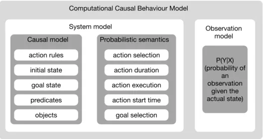
activity and goal recognition. Section3presents the idea behind CSSMs and we discuss a concrete
60
implementation of CSSMs, called Computational Causal Behaviour Models, that we use in this work.
61
Section4describes the experimental setup and the model development while Section5presents
62
the results. The work concludes with a discussion and outline of future work in Sections6and7
63
respectively.
64
2. Related Work
65
To be able to reason about one’s cooking and eating behaviour and its implications on their
66
health, a system has to be able to infer information about the person’s behaviour from observation by
67
means of sensors. To this end, current work distinguishes between Activity Recognition (AR), goal
68
recognition (GR) and Plan Recognition (PR) [14]. Activity recognition is known as the task of inferring
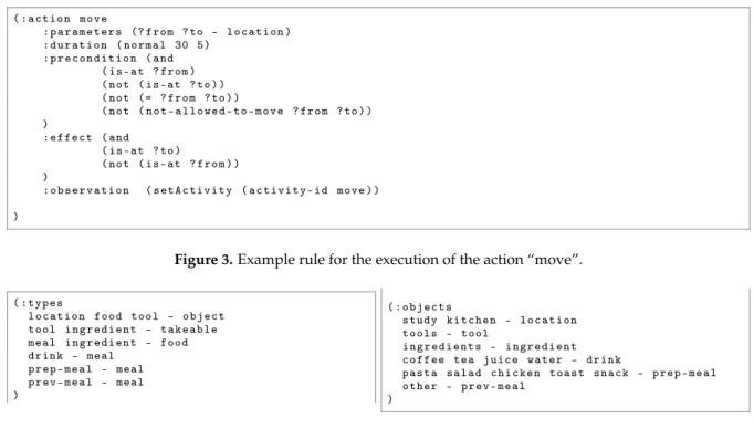
69
the user’s current action from noisy and ambiguous sensor data, while GR deals with recognising the
70
goal the person is pursuing. Plan recognition, in contrast, aims to infer the action sequence leading
71
to a goal under question by using (partial) action observations. Plan recognition can be considered
72
as the combination of activity and goal recognition. In other words, PR recognises both the person’s
73
sequence of actions and goals they follow.
74
The term “behaviour recognition”, on the other hand, refers to the overall process of activity, goal,
75
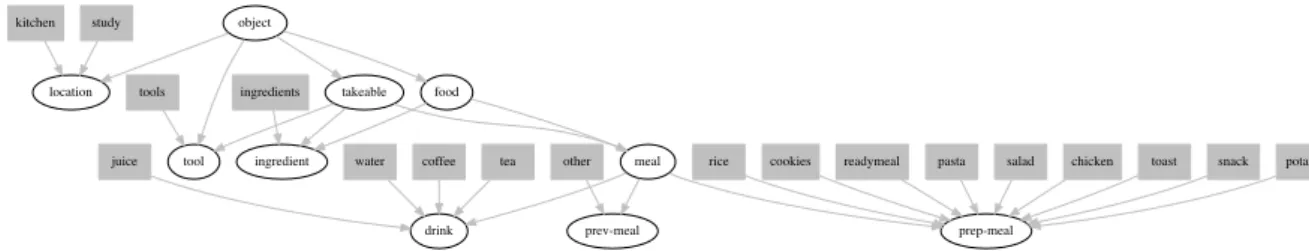
and plan recognition [15]. In the framework of behaviour recognition we refer to “actions” as the
(a) (b) (c) 1 2 T X Y X Y X1 Y1 X2 Y2 XT YT
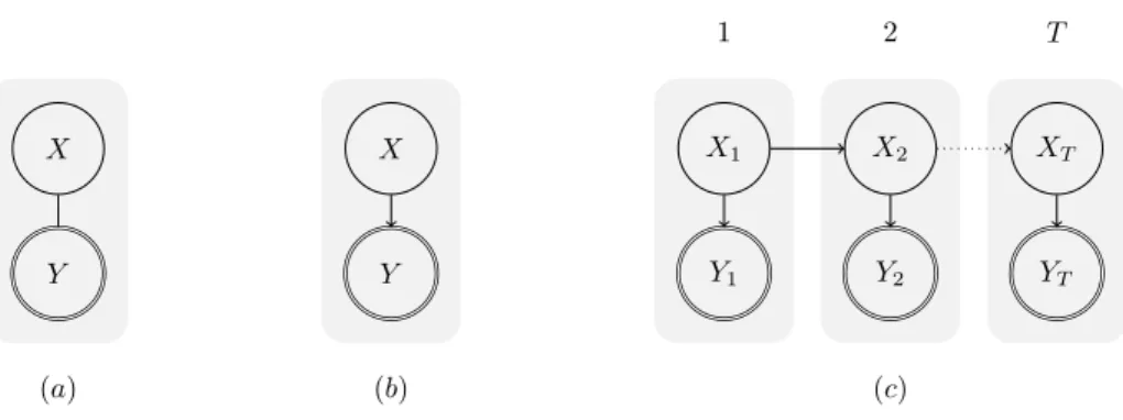
Figure 1. Graphical representation of three different types of classifier. X represents a hidden state and Y an observation that is used to conclude information about X. (a) discriminative classifier, (b) generative classifier without temporal knowledge, (c) generative classifier with temporal knowledge (figure adapted from [16]).
primitive actions constituting a plan. A plan is then a sequence of actions leading to a certain goal1.
77
In difference to typical AR terminology, where actions can build up complex parallel or interleaving
78
activities, here we consider plan to be complex activity built up of sequentially executed actions. Based
79
on this definition, we introduce the general model of sensor based behaviour recognition which has
80
the objective to label temporal segments by use of observation data.
81
From the inference point of view, the aim of behaviour recognition is to estimate a hidden variable
82
X from an observable variable Y. Figure1(a) provides a graphical illustration of this task. Here, the
83
hidden variable X represents the activity of the human protagonist. With respect to the probabilistic
84
structure, two fundamentally different approaches to behaviour recognition exist [17]: discriminative
85
and generative classifiers. While discriminative classifiers model the conditional probability P(X|Y),
86
generative classifiers model the joint probability P(X, Y). In other words, discriminative classifiers
87
map the observation data to activity labels directly [17], while generative classifiers allow to exploit
88
the causal link between the system’s state X and the observation Y by factoring the joint probability
89
into P(X, Y) =P(Y|X)P(X). A graphical representation of generative models is provided in Figure1
90
(b). The representation allows to include prior knowledge about the dynamics of the underlying
91
process. Furthermore, experiences can often be used to establish the sensor model P(Y|X)[18, p.5].
92
[19] provide a detailed overview of methods for activity recognition. Typical approaches include
93
decision trees [20], support vector machines [21,22], or random forests [23,24].
94
By including further knowledge about the temporal structure of the activities, a transition model
95
P(Xt|Xt−1)can be introduced to provide temporally smoothed estimates of the activities. This is 96
illustrated in Figure1(c). Generally, temporal generative models (e.g. Hidden Markov Models (HMM))
97
do not raise any restrictions to the possible sequences of activities, which allows the estimation of
98
sequences that are impossible from the viewpoint of causality. Then, to reason about the causally valid
99
action sequences, we need to use plan recognition (PR) approaches. The literature provides different
100
overviews of plan recognition [14,25–28].
101
From the modelling viewpoint, two different approaches exist for restricting the set of possible
102
sequences. The first approach is to enumerate all possible sequences (plans) in a plan library [29].
103
However, the plan library has to be created manually, which is a tedious task due to the high number
104
1 Note that there is some variation in the interpretation of the term “activity recognition” across different works. For example,
the authors in [9] refer to activity recognition as the process of recognising coarse-grained complex activities (e.g. “prepare
breakfast”, “take a shower”, etc.) They however do not recognise the sequence of fine-grained actions needed to complete these activities. In our work, we consider the recognition of these fine-grained actions as “activity recognition”, the recognition of the correct sequence of fine-grained actions as “plan recognition”, and the recognition of the overall complex activity as “goal recognition”.
Table 1.Existing CSSMs applied to activity and goal recognition problems. Appr oach plan rec. durations action sel. pr obability
noise latentinfinity simulationmultiplegoals unscriptedscenario
[31] no [10] yes [33] no [13] no [12] no [34] yes [11] yes [35] yes [36] yes
feature not included feature included
of action sequences [30]. As pointed in [12], “library-based models are inherently unable to solve
105
the problem of library completeness caused by the inability of a designer to model all possible
106
execution sequences leading to the goal”. This is especially true in real world problems where the
107
valid behaviour2variability can result in models with millions of states and execution sequences.
108
A second approach to introducing restrictions to the set of causally valid action sequences is to
109
employ a structured state representation of X and generate only action sequences that are causally
110
valid with respect to this state. This technique is also known as inverse planning [31], as it employs
111
ideas from the domain of automated planning to infer the action sequence of a human protagonist.
112
This technique is, for instance, used by [32] and [11].
113
To cope with behaviour variability, some works introduce the use of computational state space
114
models (CSSM). CSSMs allow modelling complex behaviour with a lot of variability without the need
115
of large training datasets or manual definition of all plans, [10,11]. CSSMs describe the behaviour in
116
terms of precondition-effect rules and a structured state representation to synthesise possible action
117
sequences. The manually implemented model is very small as it requires only a few rules to generate
118
different sequences of possible actions. This is done through the causal relations defined in the rules.
119
Note that this is an alternative to manually defining all possible action sequences, or using large
120
training datasets to learn them. In addition, some CSSMs combine their symbolic structure with
121
probabilistic inference engines allowing them to reason even in the presence of ambiguous or noisy
122
observations [12,13].
123
Table1lists different works on CSSMs. For example, most of them make simplifying assumptions
124
of the environment in order to perform plan recognition. Most do not make use of action durations.
125
In real world, however, actions have durations and this makes the inference problem more complex.
126
Many works assume perfect observations, which is not the case in real world problems where the
127
sensors are typically noisy and there are missing observations. Also, most of the works assume that
128
there is only one goal being followed. In real world scenarios it is possible that the goals change over
129
time. Presently, CSSMs have been applied to problems in scripted scenarios. Such settings limit the
130
ability to investigate behaviour complexity and variability that is usually observed in everyday life.
131
There is still no solid empirical evidence that CSSMs can cope with the behaviour variability observed
132
in real world everyday activities3. Additionally, presently CSSMs have been used for recognising
133
2 We have to note that by “valid” we mean any causally correct sequence of actions. This does not necessarily mean that
the behaviour is also rational from a human point of view. “Causally correct” here indicates that the sequence of actions is physically possible (e.g. a person has to be at a given location to execute the action at this location, or an object has to be present for the person to interact with this object, etc.).
3 Note that CSSMs have been applied to the problem of reconstructing the daily activities in home settings [37]. This analysis,
however, is very coarse-grained and does not address the problem of reasoning about the fine-grained activities and goals within a certain task, e.g. while preparing a meal.
action rules initial state goal state action selection action duration action execution Causal model Probabilistic semantics
Computational Causal Behaviour Model
System model Observation
model P(Y|X) (probability of an observation given the actual state) action start time
goal selection predicates
objects
Figure 2.Elements of a Computational Causal Behaviour Model.
the goal only in scenarios with simulated data [10,11]. In other words, it is unclear whether these
134
approaches are able to reason about the user behaviour when the user is not following a predefined
135
script or agenda.
136
In a previous work, we showed preliminary results of a CSSM approach called Computational
137
Causal Behaviour Models (CCBM), which reasons about one’s activities in real cooking scenarios [1,38].
138
In this work, we extend our previous work by providing detailed information on the approach and the
139
developed model. We show that our model is able to perform goal recognition based on both multiple
140
and single “pooled” goals. We also present a detailed empirical analysis on the model performance, the
141
effect of the sensors on the performance, and we compare the proposed approach with state-of-the-art
142
Hidden Markov Model for PR. Finally, we provide a discussion on the effect of adding the person’s
143
position extracted from video data on the model performance.
144
3. Computational Causal Behaviour Models
145
The previous section introduced the concept of behaviour recognition and illustrated that CSSMs
146
provide a convenient approach by bridging the gap between activity recognition and plan recognition.
147
This section further extends these concepts and gives an introduction to Computational Causal
148
Behaviour Models, a framework for sensor based behaviour recognition based on the principle of
149
CSSMs. The description is based on the dissertation of F. Krüger [16]. Figure2describes the CCBM
150
elements.
151
CCBM provides a convenient way to describe sequences of human actions by means of computable
152
functions rather by providing plan libraries to provide all possible sequences. From the viewpoint
153
of probabilistic models, as introduced in Section2, CCBM allows to specify the temporal knowledge
154
of human behaviour — the system model P(Xt|Xt−1). To this end, CCBM employs a causal model, 155
which uses precondition and effect rules in order to describe the system dynamics. Beside the system
156
model, inference from noisy observations requires an observation model, which basically describes
157
the relation between the sensor observation Y and the system’s state X. CCBM uses a probabilistic
158
semantic to cope with uncertainties resulting from noisy sensor observations and the non-deterministic
159
human behaviour. In the following these concepts are describes in more detail.
160
3.1. Causal Model
161
As described earlier, CSSMs rely on the idea of plan synthesis. A model based description [39] is
162
employed to describe the state space and possible actions. A state is described by predicates, where
163
each represents a property of the environment such as the current position of the person, or whether
164
the person is hungry or not. Actions are described by means of preconditions and effects with respect
( : a c t i o n m o v e : p a r a m e t e r s (? f r o m ? to - l o c a t i o n ) : d u r a t i o n ( n o r m a l 30 5) : p r e c o n d i t i o n ( and ( i s - a t ? f r o m ) ( not ( i s - a t ? to ) ) ( not (= ? f r o m ? to ) ) ( not ( n o t - a l l o w e d - t o - m o v e ? f r o m ? to ) ) ) : e f f e c t ( and ( i s - a t ? to ) ( not ( i s - a t ? f r o m ) ) ) : o b s e r v a t i o n ( s e t A c t i v i t y ( a c t i v i t y - i d m o v e ) ) )
Figure 3.Example rule for the execution of the action “move”.
( : t y p e s l o c a t i o n f o o d t o o l - o b j e c t t o o l i n g r e d i e n t - t a k e a b l e m e a l i n g r e d i e n t - f o o d d r i n k - m e a l p r e p - m e a l - m e a l p r e v - m e a l - m e a l ) ( : o b j e c t s s t u d y k i t c h e n - l o c a t i o n t o o l s - t o o l i n g r e d i e n t s - i n g r e d i e n t c o f f e e tea j u i c e w a t e r - d r i n k p a s t a s a l a d c h i c k e n t o a s t s n a c k - p r e p - m e a l o t h e r - p r e v - m e a l )
Figure 4.Example definition of types and their concrete objects for the cooking problem.
to a structured state. While the preconditions restrict the application of actions to appropriate states,
166
the effects describe how the state is changed after executing an action. In case of CCBM, the causal
167
model employs a PDDL-like4notation to describe the action rules, the initial and goal states, and the
168
concrete objects in the environment. Figure3shows an example of a PDDL-like rule for the action
169
“move”. The rule represents an action template that can be grounded with different parameters. For
170
example, the action template “move” can be grounded with two parameters of type “location”5. The
171
template then incorporates its rules in terms of preconditions and effects. The preconditions describe
172
the constraints on the world in order for an action to become executable, while the effects describe how
173
the execution of this action changes the world. They are defined in terms of predicates that describe
174
properties of the world. Apart from the preconditions and effects, an action template has a duration (in
175
this case a normal distribution with a mean of 30 and a standard deviation of 5), and an “:observation”
176
clause that maps the high level action to the observation model. Apart form the action templates, the
177
objects in the environment and their types are expressed in a PDDL-like notation. Figure4shows
178
the definition of the types and objects for the cooking problem. For example, the objects “study” and
179
“kitchen” are from type “location” and the type “location” has a parent type “object”. This notation
180
builds up a hierarchy with the concrete objects at the bottom and the most abstracted class at the top.
181
A graphical representation for this structure can be seen in Figure7.
182
The action templates together with the objects generate a symbolic model that consists of actionsA,
183
statesS, ground predicatesP, and plansB. The setAof grounded actions is generated from the action
184
templates by grounding a template with all possible concrete objects. The setPof grounded predicates
185
is generated by grounding all predicates with the set of all possible objects. A state s∈ Sis defined as a
186
combination of all ground predicates and describes one particular state of the world. For a state s∈ S,
187
each state describes one possible combination of the actual values of the ground predicates. Imagine
188
we have a model, which has 3 predicates and each of these predicates can have the value true or false.
189
One possible state will have the following reprsentation s= (pr1 := true, pr2 := true, pr3 := false). 190
4 Planning Domain Definition Language [40].
t t− 1 Dt−1 Vt−1 St−1 At−1 Ut−1 Wt−1 Zt−1 Gt−1 Dt Vt St At Ut Wt Zt Gt Xt Xt−1 Yt Yt−1
Figure 5.DBN structure of a CCBM model. Adapted from [13].
ThenSrepresents the set of all such predicate combinations, i.e. all states that are reachable by applying
191
any sequence of action on the initial state. We can reach from one state s to another s0by applying an
192
action a∈ Ain s. We then say that s0is reachable from s by a. The initial state s0, is the state of the 193
world at the beginning of the problem. Apart from the initial state, another important subset of states
194
is the one containing the goal statesG⊆ S.Gis basically the set of states containing all the predicates
195
that have to be true in order to reach the goal the person is following.B ={p1, . . . , pn}is the set of all 196
possible execution sequences (or plans) starting in the initial state and reaching a goal state. For a plan
197
pi= (a1, . . . , am)that leads to a goal g⊆ Gand an initial state s0∈ S, we say that piachievesG, if for
198
a finite sequence of actions ajand a state sl ∈ G, sl =am(· · ·a2(a1(s0))· · · ).Bcorresponds to a plan
199
library in approaches that manually define the possible plans [29]. A plan library will then contain
200
all possible valid plans (either manually built in library-based approaches or generated from rules in 201
approaches such as CCBM). 202
3.2. Probabilistic Semantics
203
As introduced in Section2, a generative probabilistic model with temporal knowledge is modelled
204
by two random variables X and Y at different time steps, which represent the belief about the system’s
205
state and the sensor observation. In order to reason not only about the state, but also about the
206
action being executed by the person, the state X is further structured. As can be seen in Figure5, the
207
system state X is structured into the following random variables S, A, G, D, and U, each representing
208
a different aspect of the state. Similarly the observation Y is structured into Z, W, and V, each
209
representing different types of sensory observation.
210
From the illustration it can be seen, that the state X at time t depends on the state at time t−1. The transition model describes this dependency through the probability P(Xt|Xt−1)of observing that
we are in a state X given that the the previous state was Xt−1. We call this model a system model.
Since the state X is a five-tuple(A, D, G, S, U), this can be rewritten as:
p(Xt|Xt−1) =p(At, Dt, Gt, St, Ut|At−1, Dt−1, Gt−1, St−1, Ut−1, Vt, Vt−1) (1)
Here, the random variable A represents the action (from the setA) that is currently executed by
211
the human protagonist while trying to achieve the goal G (from the setG). The current state of the
212
environment is represented by S (from the setS). The variables U and D represent the starting time of
213
the current action and signal whether the action should be terminated in the next time step. Finally, the
214
variables V, W, and Z reflect observations of the current time, environment, and action, respectively.
By exploiting the dependencies from the graphical model, this transition model can be simplified into five sub-models, each describing the dependency of one element of the state.
p(St|At, Dt, St−1) Iaction execution model (2)
p(At|Dt, Gt, At−1, St−1) Iaction selection model (3)
p(Ut|Dt, Ut−1, Vt) Iaction start time model (4)
p(Dt|At−1, Ut−1, Vt, Vt−1) Iaction duration model (5)
p(Gt|Xt−1) Igoal selection model (6)
The action execution model describes the application of the actions to a state and the resulting state. This sub-model basically implements the effects of the action description. For this purpose, the resulting state is determined based on the current state, the action to be executed, and whether the current action is finished or not. More formally,
p(st|at, dt, st−1) = 1, if dt=false∧st=st−1; 1, if dt=true∧st=at(st−1); 0, otherwise. (7)
Depending on the value of dt, either the system’s state remains untouched, or the new state stis set to 216
the results of applying the selected action atto the current state st−1. While the action execution model 217
generally allows the usage of non-deterministic effects (i.e. the outcome of an action is determined
218
probabilistically), CCBM’s deterministic effects are considered sufficient in order to model the human
219
protagonist’s knowledge about the environment.
220
Both, the action start time and the action duration model implement the fact that actions executed by human protagonists consume time. While the first model basically “stores” the starting time of the current action, the second model determines whether the action that is currently executed should be terminated or not. From the probabilistic viewpoint, the action start time model is rather simple. The value of utis set to the current time t if a new action is selected, otherwise the value is copied from the
previous time step. More formally,
p(ut|dt, ut−1, vt) =
(
1, if(dt=false∧ut=ut−1)∨ (dt=true∧ut=vt);
0, if(dt=false∧ut6=ut−1)∨ (dt=true∧ut6=vt).
(8)
The action duration model employs the start time of an action to determine the termination by use of an action specific duration function (provided by the CDF F):
p(dt|at−1, ut−1, vt, vt−1) = F(vt|at−11, u−tF−1(v)−F(vt−1|at−1, ut−1)
t|at−1, ut−1) (9)
Objective of the goal selection model is to provide a mechanism to model the rational behaviour of the human protagonist. While different approaches in the literature allow changes of the goal (see for instance [31] or [41]), CCBM is based on the assumption that once a goal is selected it is not changed. Similar as for the deterministic action execution, this assumption is based on the complete and static knowledge of the human protagonist. This means that the goal is chosen at time t=0 and copied from the previous time step afterwards.
p(gt|gt−1, st−1, at−1, dt−1, ut−1) =
(
1, if gt =gt−1
To reflect the human protagonist’s freedom to choose an action, the action selection model
221
provides a probability distribution over possible actions. This includes two aspects:
222
1. goal-directed actions are preferred, but
223
2. deviations from the “optimal” action sequence are possible.
224
Whenever the previous action has been terminated, a new action has to be selected.
p(at|dt, gt, at−1, st−1) = γ(at|gt, at−1, st−1), if dt=true 0, if dt=f alse∧at6=at−1 1, if dt=f alse∧at=at−1 (11)
This is done by the action selection function γ, which is implemented based on log-linear models. This allows to include different factors into the action selection mechanism.
˜ γ(at|gt, at−1, st−1) =exp(
∑
k∈K λkfk(at, gt, at−1, st−1)) (12) γ(at|gt, at−1, st−1) =Z1γ˜(at|gt, at−1, st−1) (13) Z=∑
a∈A ˜ γ(at|gt, at−1, st−1) (14)Here fkis the feature used for the action selection with k ={1, 2}. f1is based on the goal distance 225
[42], while f1uses a landmarks-based approximation of the goal distance [43]. The distance in f1is 226
determined by an exhaustive process, which could be infeasible in very large state spaces. For that
227
reason f2uses approximation based on the predicates that have to be satisfied to reach the goal. The 228
weight λkallows the adjust the influence of the particular heuristic to the action selection model. 229
3.3. Observation Model
230
The connection between the system model and the observations is provided through the observation model. It gives the probability p(Yt=yt|Xt=x)of observing an observation y given a
state x. As illustrated in Figure5the random variable Y is structured into Z, W, and V, representing sensors observation of actions (e.g. movement of a person), the environment (e.g. whether a cupboard is open or closed) and the current time. While the observation model itself is not part of the causal model, but has to be provided separately, the :observation clause in the action template is used to map the specific functions from the observation model to the high level system model (see Figure3). The :observation provides the observation model with information about the current state X, such as the action currently executed or the environment state. Objective of the observation model is to provide the probability of the sensor observation given the action a∈ Aand state s∈ S.
P(Yt|Xt) =P(Zt|At)P(Wt|St) (15)
While there are no restrictions to way, in which this probability is computed, here we use an observation
231
model that incorporates a decision tree. More information about the implementation of the system
232
and observation models can be found in [44].
233
4. Experimental Setup and Model Development
234
4.1. Data Collection
235
To investigate whether CSSMs are applicable to real word scenarios, we used a sensor dataset
236
recorded in real settings. The dataset consists of 15 runs of food preparation and eating activities. The
237
dataset was collected in a real house rented by the SPHERE project (a Sensor Platform for HEalthcare
Figure 6.The SPHERE house at the University of Bristol and the kitchen setup.
in a Residential Environment) [45]. SPHERE is an interdisciplinary research project aiming to assist
239
medical professionals in caring for their patients by providing a monitoring solution in home settings
240
[45]. The SPHERE House is a normal 2-bedroom terrace in Bristol (UK) into which has been installed
241
the full SPHERE system for testing, development and data collection. The SPHERE system consists of a
242
house wide sensor network which gathers a range of environmental data (such as temperature, humidity,
243
luminosity, motion), usage levels (water and electricity), and RGB-D features from depth cameras in the
244
downstairs rooms [46]. The system also has support for a wearable sensor, used for location, heart-rate
245
and an on-board accelerometer, although this was not used for this dataset due to hygiene concerns.
246
For this work, binary cupboard door state monitoring was also added in the house kitchen to provide
247
additional domain relevant data [47]. A head-mounted camera was used during the data collection to
248
provide a point-of-view for each participant allowing for easier annotation of the observations. Due to
249
extensive consultation with members of the public and medical professionals, the SPHERE system
250
strikes a balance between protecting the privacy of the occupants and providing useful clinical data.
251
Figure6shows the SPHERE house and the kitchen setup.
252
Each participant was given ingredients that they had requested and asked to perform two or three
253
cooking activities of their choice without any set recipe or other restrictions. They were encouraged
254
to act naturally during the recordings, which lead to a range of behaviours, for example leaving the
255
kitchen for various reasons, preparing drinks as desired and using personal electrical devices when
256
not actively cooking. This led to various meals, both in terms of preparation time and complexity,
257
and a range of exhibited behaviours. Table2shows the different runs, the meals and drinks that were
258
prepared and whether they have been classified as healthy for the purposes of this work. It also shows
259
the length of the task in terms of time steps after the data was preprocessed (see Section4.2). The
260
resulting dataset can be downloaded from [48]. Note that this dataset does not contain the RGB-D data
261
from the depth cameras as this is not stored by the system for privacy reasons. Bounding boxes of
262
humans in the scene, generated by the system from the RGB-D in real time, are included and used in
263
this work to evaluate whether the information from the cameras improves model performance (see
264
Section5.2).
Table 2.Types of meal and length of execution sequence in a dataset. “Number of Actions” gives the discrete actions required to describe the sequence (i.e. it gives the number of actions executed during the task). “Time” gives the duration of the recording in time steps.Time steps are calculating by using a sliding window over the data, which is originally in milliseconds (see Section4.2).“Meal” gives the eventual result of the food preparation.
Dataset # Actions Time Meal
D1 153 6502 pasta (healthy), coffee (unhealthy), tea (healthy)
D2 13 602 pasta (healthy)
D3 18 259 salad (healthy)
D4 112 3348 chicken (healthy)
D5 45 549 toast (unhealthy), coffee (unhealthy)
D6 8 48 juice (healthy)
D7 56 805 toast (unhealthy)
D8 21 1105 potato (healthy)
D9 29 700 rice (healthy)
D10 61 613 toast (unhealthy), water (healthy), tea (healthy) D11 85 4398 cookies (unhealthy)
D12 199 3084 ready meal (unhealthy), pasta (healthy)
D13 21 865 pasta (healthy)
D14 40 1754 salad (healthy)
D15 72 1247 pasta (healthy)
4.2. Data Processing
266
The dataset was recorded in JSON format. After converting it into column per sensor format, the
267
procedure generated multiple rows with the same timestamp (in milliseconds). To remove redundant
268
data, we combined rows with the same timestamp given that there was only one unique value for
269
a sensor type. Furthermore, the action class was added for each row in the data. As the conversion
270
generates some undefined values (due to the different frequencies of data collection for each type
271
of sensor), time steps with undefined values for a particular sensor were replaced with the nearest
272
previous value for that sensor. Apart from collecting the sensors’ values at a certain sampling rate, the
273
value was also recorded when a change in the sensor’s state was detected. This ensures that replacing
274
undefined values with the previous one, will not result in transferring incorrect values when the
275
sensor changes its state. To reduce the impact of ambiguous observations on the model performance,
276
we applied a sliding window for all sensors with overlapping of 50%. We used a window size of 5.
277
We summarised the values in a window by taking the maximum for each sensor. A larger window
278
resulted in removing certain actions from the dataset. For that reason we chose the window size of 5
279
steps. This still produced actions with equivalent observations but reduced their number. The length
280
of the resulting execution sequences in time steps can be seen in Table2.
281
4.3. Data Annotation
282
In order to obtain the annotation, an action schema and ontology were developed and used for
283
the annotation and the CCBM model design considerations. The ontology contains all elements in
284
the environment that are relevant for the annotation and the model, while the action schema gives
285
the restrictions on which actions can be applied to which elements in the environment. Note that
286
the proposed action schema is more fine-grained than other existing works on AR in home settings
287
(e.g. see [37,49]). This could be partially explained with the fact that sensors are unable to capture
288
fine-grained activities leading to the development of action schema on the sensors’ granularity level
289
[50]. In this work, we follow the assumption that we need an action schema on the granularity level
290
of the application domain, so we are not guided by the sensors’ granularity. In other words, we can
291
produce annotation that is not captured by the sensors. To produce the annotation, we followed the
292
process proposed in [51,52].
4.3.1. Ontology
294
The ontology represents the objects, actions, and their relations that are relevant for the problem.
295
The actions in the ontology refer to the meal they are contributing to (e.g. “get ingredient pasta” means
296
“get the ingredient needed for preparing pasta”). The action schema used in the model are shown in
297
Table3. They provide the rules for applying actions on elements in the environment. For example, Table 3.The actions schema for the ontology.
1) (move <location> <location>) 5) (eat <meal>) 2) (get <item> <meal>) 6) (drink <meal>) 3) (put <item> <meal>) 7) (clean)
4) (prepare <meal>) 8) (unknown)
298
prepare can be applied only on element of type meal. In Table3, location and item represent sets of
299
objects, necessary for achieving the task, while meal refers to the goal of preparing a certain type of
300
meal. The concrete locations, items and meals can be seen in Table4. Here the get, put and prepare
301
actions do not take into account the location where the meal is being prepared but rather the type
302
of meal as a goal. Beside the goal oriented actions, the ontology also has an unknown action, which
303
describes actions that do not contribute to reaching the goal. Figure7shows the objects’ hierarchy for
object location food tool takeable meal ingredient
drink prev-meal prep-meal study
kitchen
coffee tea
juice water other rice cookies readymeal pasta salad chicken toast snack potato ingredients
tools
Figure 7.The relevant elements in the environment represented as hierarchy. Rectangles show objects; ellipses describe the object types;arrows indicate the hierarchy or “is-a” relation (the arrow points to the father class). Figure adapted from [38].
304
the action schema. The rectangles show the object used in the experiment, while the ellipses depict the
305
object types. The types are the same as those in Table4.
306
4.3.2. Annotation
307
Based on the ontology, 15 datasets were annotated using the video logs from the head mounted
308
camera and the ELAN annotation tool [53]. The process proposed in [51] was used, ensuring that
309
the resulting annotation is syntactically and semantically correct. Figure5shows an example of the
310
annotation, where the time indicates the start of the action in milliseconds. The annotation has then
311
been mapped to the processed sensor data, where the time is no longer in milliseconds but in time
312
steps.
313
The length of the annotation sequences after synchronising with the sensor data (with and without
314
timing) can be seen in Table2. The types of meals are also listed there. The annotation was later used
315
to simulate data for the experiments reported in [38]. It was also used as a ground truth in this work
316
during the model evaluation as well as for training the observation model for the CCBM.
317
Table 4.Object sets in the ontology.
Meal chicken, coffee, cookies, juice, pasta, potato, readymeal, rice, salad, snack, tea, toast, water, other
Item ingredients, tools Location kitchen, study
Table 5.Excerpt of the annotation for run D1. Time here is given in milliseconds. Time Label
1 (unknown)
3401 (move study kitchen) 7601 (unknown)
10401 (prepare coffee) 31101 (unknown) 34901 (clean) 47301 (unknown) 52001 (get tools pasta) 68001 (get ingredients pasta) 86301 (prepare pasta) 202751 (get tools pasta) 221851 (get ingredients pasta) 228001 (prepare pasta)
4.4. Model Development
318
To develop the model, we follow the process proposed in [12]. It consists of developing the causal
319
model and the observation model, then defining the different heuristics for action selection and finally
320
identifying appropriate action durations.
321
4.4.1. CCBM Models
322
Causal model: We first developed 15 specialised models, which were fitted for each of the
323
15 execution sequences (we call these models CCBMs). More specifically, for all 15 models the 324
same precondition-effect rules were used, but the initial and goal states differed so that they could
325
accommodate the specific for each meal situation. We built the specialised models only for comparison
326
purpose, as we wanted to evaluate whether our general model performs comparable to specialised
327
models, which are typically manually developed in approaches relying on plan libraries. We also
328
developed a general model, able to reason about all sequences in the dataset and allows performing GR
329
(we call this model CCBMg). The model uses the action schema presented in Figure3and can label the 330
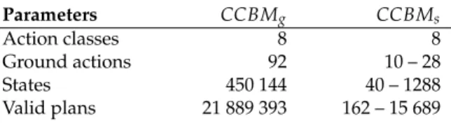
observed actions as one of the classes clean, drink, eat, get, move, prepare, put, unknown. The model size Table 6.Parameters for the different models.
Parameters CCBMg CCBMs Action classes 8 8 Ground actions 92 10 – 28 States 450 144 40 – 1288 Valid plans 21 889 393 162 – 15 689 331
in terms of action classes, ground actions, states, and plans for the different model implementations
332
can be seen in Table6. Here, “action classes” shows the number of action types in the model, “ground
333
actions” gives the number of unique action combinations based on the action schema in Table3,
334
“states” gives the number of S-states the model has, and “valid plans” provides the number of all
335
valid execution sequences leading from the initial to one of the goal states. The general model has a
336
larger state space and a larger set of plans. This allows coping with behaviour variability, however, it
337
potentially reduces the model performance in contrast to the over-fitted specialised model.
338
Goals in the model: To test whether the approach is able to reason about the observed behaviour, we
339
modelled the different type of behaviour as different goals. As we are interested not only in the type of
340
meal the person is preparing, but also what influence it has on the person’s health, we integrated two
341
types of goals:
342
1. type of meal being prepared. Here we have 13 goals, which represent the different meals and
343
drinks the person can prepare (see Table4);
2. healthy / unhealthy meal / drink (4 goals). Here we made the assumption that coffee, toast, and
345
ready meals are unhealthy, while tea and freshly prepared meals are healthy (see Table2). This
346
assumption was made based on brainstorming with domain experts.
347
Note, that although the goals could also be interpreted as actions or states, in difference to AR
348
approaches, in GR we are able to predict them before they actually happen.
349
Duration model: The action durations were calculated from the annotation. Each action class
350
received probability that was empirically calculated from the data. The probability models the duration
351
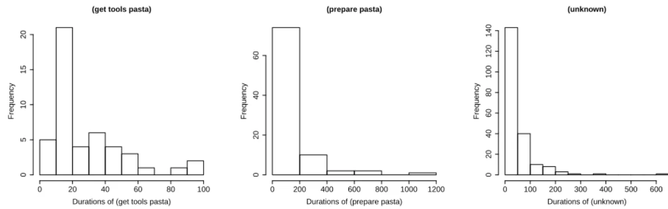
of staying in the one state. Figure8shows selected examples of the frequency of action durations for a
(get tools pasta)
Durations of (get tools pasta)
Frequency 0 20 40 60 80 100 0 5 10 15 20 (prepare pasta)
Durations of (prepare pasta)
Frequency 0 200 400 600 800 1000 1200 0 20 40 60 (unknown) Durations of (unknown) Frequency 0 100 200 300 400 500 600 0 20 40 60 80 100 120 140
Figure 8.Frequency of the durations of some actions in the dataset.
352
given action.
353
Observation model: The observation model P(y|x)has been obtained by a learning-based approach
354
as follows. We trained a decision tree (DT) based on the action classes. The output of the DT is for
355
each time step, a distribution of the action class, given the current observation. This output has been
356
used as a high-level observation sequence that is used to update the state prediction of the CCBM, by
357
weighting each state by the probability of the corresponding action class, as indicated by the DT. The
358
DT was applied to the following sensors:
359
• fridge electricity consumption: for this sensor we expect to see more electricity consumption when
360
the door of the fridge is open, which will indicate an ingredient being taken from the fridge;
361
• kitchen cupboard sensors (top left, top right, sink): show whether a cupboard door is open, which
362
could indicate that an ingredient or a tool has been taken from the cupboard;
363
• kitchen drawer sensors (middle, bottom): as with the cupboard sensors, provide information whether
364
a drawer has been opened;
365
• temperature sensor: measures the room temperature and increasing temperature can potentially
366
indicate the oven or stoves being used;
367
• humidity sensor: measures the room humidity and increased humidity can indicate cooking
368
(especially when boiling water for the pasta);
369
• movement sensor: provides information whether a person is moving in the room. This is useful
370
especially for the eating actions, when the person leaves the kitchen and eats in the study;
371
• water consumption (hot and cold): shows the water consumption in the kitchen. This is useful
372
especially in the cleaning phase.
373
• kettle electricity consumption: as with the fridge, we expect to see more electricity consumption
374
when the kettle is on and somebody is boiling water.
375
• depth cameras: the position of the person was estimated through the depth cameras. We expected
376
that adding the position will increase the model performance.
377
We trained two types of observation models with DT:
1. OMo: We used all data to train the OM and the the same data to test the model (o denotes 379
“optimistic”). This is an over-fitted model and we assume it should provide the best performance
380
for the given system model and sensor data. Although this model is not realistic, it gives us
381
information about the capabilities of the approach under optimal conditions.
382
2. OMp: We used the first run for training and the rest to test the model (p denotes “pessimistic”). 383
We chose the first run as it is the only one containing all actions. This observation model gives us
384
information about the performance of the system model in the case of very fuzzy observations.
385
4.4.2. Hidden Markov Model
386
In order to compare the CCBM approach to the state of the art, we also built a hidden Markov
387
model (HMM) both for activity and goal recognition. The number of hidden states in the HMM equals
388
the number of action classes. Figure9shows a graphical representation of the modelled HMM.
clean drink eat get move prepare put unknown
Figure 9.The HMM used for activity recognition. Each state represents an action class. Thicker lines indicate higher transition probabilities.
389
The HMM has a transition matrix as well as prior probabilities for each state. We empirically
390
estimated the transition matrix from the annotation of the training data by counting the number of
391
state transitions. The state prior probabilities are based on the number of times a state appears in the
392
training data. Two different transition models have been examined:
393
• estimating the transition model from the data of all runs (general HMM, we call this model
394
HMMg); 395
• estimating the transition model separately for each run (specialised HMM, we call this model
396
HMMs). 397
For the HMMs we used the same two observation models as with the CCBM model.
398
Goal Recognition
399
The HMM has been used for goal recognition as proposed in [16]. This means, an HMM has been
400
built for each possible goal. Each HMM has been trained using all runs where this goal occurs. These
401
HMMs have been combined by introducing a common start state. The transition probabilities from the
402
start state to the states of the sub-models are the normalised priors of the sub-model states. Note that
403
the sub-models can have different number of states, when not all action classes occur in a run. This
404
type of HMM is known as joint HMM [54]. This way, each state in the joint HMM is a tuple (action
405
class, goal) and the probability of a goal is computed by marginalising over all states with the same
406
goal.
407
4.5. Evaluation Procedure
408
To select the best combination of sensors for behaviour recognition and to evaluate the models’
409
performance, the following experiments were conducted:
1. feature selection of the best combination of sensors. This experiment was performed to select the
411
sensors that at most contribute to the model performance. The selected combination was later
412
used when comparing the CCBM and HMM models;
413
2. activity recognition of the action classes with DT, HMM, and CCBM models;
414
3. goal recognition of the types of meals and drinks as well as preparation of healthy / unhealthy
415
meal / drink.
416
4.5.1. Feature selection
417
We used the HMM for activity recognition to find the best feature combination, where by “feature”
418
we mean the type of sensor. We did two types of evaluation: we first performed activity recognition
419
with all feature combinations without the features from the depth cameras (212 =4096 combinations).
420
This feature selection was performed with OMpas the observation model and DT as classifier. OMp 421
has been chosen because it gives the most realistic assessment of the performance on new data (OMo 422
is over-fitted and selecting features with this observation model would result in an over-fitted feature
423
combination, i.e. in too many features).
424
This procedure results in accuracies for all feature combinations. We computed the accuracy using Accuracy= ∑CλC
N . (16)
Here C represents the action class. N represents all instances that are classified. λ is the number of
425
correctly recognised instances in C.
426
As we wanted to decide which features to use for the model evaluation, for each feature f we
427
calculated how much it contributes to the model performance.
428
1. We start by comparing the mean performance for the different feature combinations;
429
2. we decide that f may produce noise when the performance of the models which contain f is
430
below the accuracy of the rest of the models;
431
3. for the model comparison, choose the feature combination with the highest accuracy.
432
We performed similar procedure for all features combinations including the features from the 433
depth cameras ((215 = 32, 768 combinations)). We performed this second evaluation separately as
434
the first run (D1) does not contain the features from the depth cameras but it is the only dataset that 435
contains all action classes. For that reason we performed a leave-one-out cross validation. D1 was thus 436
removed from the evaluation. For each feature combination, we performed 14 training runs: training 437
with all of the runs except i, and evaluating the performance (accuracy) on run i. Then, the accuracy 438
was calculated as the mean accuracy of the 14 runs. 439
4.5.2. Activity recognition
440
We use factorial design for both activity and goal recognition. For the activity recognition, three
441
types of factors were examined:
442
1. algorithm:this factor considers the different approaches to be compared (DT, HMM, CCBM). The
443
decision tree was our baseline and it gives information about the performance when applying
444
only the observation model. In that sense, we expected the HMM and CCBM models to perform
445
better that the DT;
446
2. observation model:(optimistic / pessimistic);
447
3. system model:(general / specific). In the case of DT we did not have different system models.
448
The different dimensions we considered resulted in 10 models.
449
4.5.3. Goal recognition
450
Each dataset was annotated with one or several goals. Two kinds of goal annotations exist:
• Meal goals: pasta, coffee, tea, salad, chicken, toast, juice, potato, rice, water, cookies, ready meal
452
• Healthy/unhealthy goals: healthy drink, unhealthy drink, healthy meal, unhealthy meal
453
The goals for a given run can be seen in Table2.
454
CCBMs (and HMMs) normally cannot recognise multiple goals. Instead, they recognise one goal
455
for each time step. Ideally, they converge after some time, only recognising a single goal after this
456
time. To perform multi-goal recognition (as required by this scenario), we examined two strategies for
457
deriving multiple goals.
458
Multiple goals strategy: we collected all goals that have been recognised at least once by the algorithm, and compared them with the set of true goals. The performance of each dataset was estimated by Formula17.
performance(i) = |esti∩truthi| |esti|
(17) Here estiis the set of recognised goals for dataset i, and truthiis the set of true goals for dataset i. The 459
overall performance is the mean of each datasets’ performance.
460
“Pooled” goals strategy:each distinct set of goals was subsumed as a goal set. We performed
461
goal recognition with this goal set. The goal of a run is said to be recognised correctly if the goal
462
estimation of this run converged to the correct goal.
463
Furthermore, we used different types of goal priors:
464
1. uniform priors (uninformed):in this case all priors (i.e. x0) have the same probability. 465
2. informed priors:here, the correct goal has two times the likelihood than the rest of the goals.
466
When applying factorial design to the goal recognition, the activity recognition factors do not
467
apply, as each sub-HMM has been trained by using the data of all runs where the corresponding goal
468
occurs. For that reason, for the goal recognition, we examined the following factors:
469
1. algorithm(HMM / CCBM);
470
2. goal target(Meal / Healthy);
471
3. type of multigoal recognition(multiple goals / single, “pooled” goals);
472
4. prior(informed / uninformed).
473
This resulted in 16 models.
474
5. Results
475
5.1. Feature Selection without the Depth Camera Features
476
4096 combinations of sensors were evaluated and from them the best combination was selected
477
for the further experimentation. Using the procedure described in the previous section, the mean
478
accuracy of the model with and without a given feature was calculated. Figure10(left) shows the
479
results. It can be seen that the humidity sensor reduces the performance of the model the most. The
480
fridge electricity consumption, movement sensor, and temperature sensor also slightly reduce the
481
mean performance. Interestingly enough, the fridge electricity consumption and movement sensors
482
are both in the set of best performing feature combination (see Table7). This indicates that taking
483
the mean accuracy is probably not the best evaluation metric as some of the sensor combinations can
484
reduce the usefulness of a sensor that otherwise brings relevant information to the model.
485
Table7shows the 10 worst and the 10 best combinations. The best performing set of features is
486
fridge, cupboard top right, movement sensor, hot water consumption, cold water consumption with accuracy of
487
0.4332. This combination was later used in the remainder of the experiments.
488
5.2. Feature Selection with Locational Data from Depth Cameras
489
During the experiment, the position of the person estimated through depth cameras was also
490
recorded. One hypothesis we had, was that adding the position will increase the model performance.
● ● ● ● ● ● ● ● ● ● ● ● ● ● ● ● ● ● ● ● ● ● ● ● 0.32 0.34 0.36 0.38 0.40
HUM PIRTEMP WCD WHT cupboardSink cupboardT opLeft cupboardT opRight drawBottomdrawMiddle fridge kettle sensor accur acy models● ● with without ● ● ● ● ● ● ● ● ● ● ● ● ● ● ● ● ● ● ● ● ● ● ● ● ● ● ● ● ● ● 0.32 0.34 0.36 0.38 0.40 HUM PIRTEMPWCD WHT cupboardSink cupboardT opLeft cupboardT opRight drawBottomdrawMiddle
fridgekettlexCoordyCoordzCoord
sensor accur acy models● ● with without
Figure 10. Mean accuracy with and without a given feature. Left: the accuracy for all feature combinations without the camera features and using the first run (D1) for training and the rest for testing. Right: the accuracy of all feature combinations including the camera features and using leave-one-out cross validation.
This hypothesis was not confirmed by the empirical results we obtained after adding the position to
492
the existing sensor data. Below we discuss the procedure for the data processing and the empirical
493
results.
494
In order to address privacy concerns about RGB-D images being stored within the SPHERE
495
system, there was a requirement for all features to be extracted at run time [46]. In order to obtain
496
the positional and tracking information of any scene elements of interest, the SPHERE system makes
497
use of a Kernelised Correlation Filter (KCF), augmented with Depth Scaling (DS-KCF) [55]. This is
498
an extremely lightweight object tracker which is capable of handling the complicated environments
499
encountered by SPHERE, while running at around 180 frames per second.
500
By using DS-KCF to obtain a 2D bounding box for an individual in frame along with the depth
501
information from the image, a 3D bounding box could be established in order to get the 3D position
502
for each person within shot. This information was stored as Cartesian coordinates, and during data
503
processing was handled in the same way as the rest of the sensor data (see Section4.2). Three new
504
columns were added for the x, y, and z position of the person extracted from the video data. To evaluate
505
whether the video data provides any additional information that increases the model performance,
506
we performed the feature selection process for all features including the depth camera features as
507
presented in Section4.5.1.
508
The 10 best and worst features are shown in Table8. It can be seen that the video data does
509
not appear in the 10 best feature combinations. For this evaluation, the best feature combination is
510
kettle electricity consumption, cupboard top left, drawer bottom, temperature, and movement. This feature
511
combination does not include any camera features. When visually inspecting the video data compared
512
to the actions from the ground truth, it became apparent that the camera data does not allow any
513
conclusions about the currently performed activity. This could be interpreted in two ways. The
514
performed activities are not related to the position of the person in the kitchen (e.g. the action “prepare”
515
can take place at different locations within the kitchen). The second interpretation is that the position
516
extracted from the camera is noisy and thus does not provide useful information for the model.
517
Figure10(right) shows the mean accuracy of all feature combinations with and without each
518
feature. This shows how much each feature contributes to the overall performance. It shows that the
519
camera features reduce the performance. Interestingly enough, in contrast to the results from Figure
520
10(left), here the movement sensor and the fridge electricity consumption improve the performance.
521
These two sensors were also used in the set of sensors selected for our experiments.
522
5.3. Activity Recognition
523
Figure11 shows the results for activity recognition. It depicts the distribution of the results
524
for a given model over all runs. The accuracy is quite similar for all algorithms. There is a slight
Table 7.Accuracies for the 10 worst and 10 best sensor combinations without the camera features. 10 worst combinations
features accuracy
fridge, drawer middle, drawer bottom, humidity, movement 0.2688 fridge, drawer middle, drawer bottom, humidity, movement, water cold 0.2691 fridge, drawer bottom, humidity, movement, water cold 0.2692 fridge, drawer bottom, humidity, movement 0.2692 fridge, cupboard top left, humidity, movement 0.2694 fridge, cupboard top left, drawer middle, humidity, movement 0.2694 fridge, humidity, movement, water cold 0.2695 fridge, drawer middle, humidity, movement, water cold 0.2695 fridge, cupboard sink, humidity, movement, water cold 0.2695 fridge, draw middle, humidity, movement 0.2695
10 best combinations
features accuracy
drawer bottom, cupboard sink, water hot, water cold 0.4307 drawer middle, drawer bottom, water hot, water cold 0.4308 cupboard top left, drawer middle, drawer bottom, water hot, water cold 0.4308 drawer middle, drawer bottom, cupboard top right, water hot, water cold 0.4308 fridge, drawer bottom, movement, water hot, water cold 0.4325 fridge, movement, water hot, water cold 0.4330 fridge, cupboard top left, movement, water hot, water cold 0.4330 fridge, draw middle, movement, water hot, water cold 0.4330 fridge, cupboard sink, movement, water hot, water cold 0.4330 fridge, cupboard top right, movement, water hot, water cold 0.4332
improvement in the recognition when using CCBMgwith OMocompared to the HMM and DT models. 526
In combination with OMp, however, there is no difference in the performance of CCBMg, HMMg, 527
HMMs, and DT. Applying CCBMs, there is improvement in the performance both when combined 528
with OMoand OMp. This improvement, however, is not significant compared to the rest of the models 529
(0.038<p value<0.187, 81<V<86 when applying Wilcoxon signed rank test with N =156). The results
OM−o OM−p dt hmmg hmms CCBM.s CCBM.g dt hmmg hmms CCBM.s CCBM.g 0.2 0.4 0.6 0.8 Accur acy
Figure 11.Activity Recognition results.OM-o refers to the optimistic observation model, OM-p to the pessimistic observation model, dt is decision tree, hmmg is the general HMM, hmms is the specialised HMM, CCBM.s is the specialised CCBM, CCBM.g is the general CCBM.
530
show that the CCBM models do not significantly improve the performance for activity recognition and
531
that the observation model has the largest effect on the accuracy. This is to be expected with regard
532
to CCBMgas the model is very general (with 21 million valid plans), which allows coping with the 533
behaviour variability but in the same time provides multiple explanations for the observed behaviour
534
6 p value of 0.038 was observed between HMM
gand CCBMs. Although it is slightly under the threshold value of 0.05, we

![Figure 5. DBN structure of a CCBM model. Adapted from [13].](https://thumb-eu.123doks.com/thumbv2/123doknet/14664779.740488/8.892.295.610.141.404/figure-dbn-structure-ccbm-model-adapted.webp)