HAL Id: tel-01253529
https://hal.inria.fr/tel-01253529
Submitted on 18 Jan 2016HAL is a multi-disciplinary open access archive for the deposit and dissemination of sci-entific research documents, whether they are pub-lished or not. The documents may come from teaching and research institutions in France or abroad, or from public or private research centers.
L’archive ouverte pluridisciplinaire HAL, est destinée au dépôt et à la diffusion de documents scientifiques de niveau recherche, publiés ou non, émanant des établissements d’enseignement et de recherche français ou étrangers, des laboratoires publics ou privés.
strategies for 3D multi-core heterogeneous architectures
Quang Hai Khuat
To cite this version:
Quang Hai Khuat. Definition and evaluation of spatio-temporal scheduling strategies for 3D multi-core heterogeneous architectures. Hardware Architecture [cs.AR]. Université de Rennes 1, 2015. English. �tel-01253529�
THÈSE / UNIVERSITÉ DE RENNES 1
sous le sceau de l’Université Européenne de Bretagne
pour le grade de
DOCTEUR DE L’UNIVERSITÉ DE RENNES 1
Mention : Traitement du Signal et Télécommunications
École doctorale MATISSE
présentée par
Quang-Hai Khuat
préparée à l’unité de recherche UMR6074 IRISA
Institut de recherche en informatique et systèmes aléatoires - CAIRN
École Nationale Supérieure des Sciences Appliquées et de Technologie
Definition and
evaluation of
spatio-temporal
scheduling strategies
for 3D multi-core
heterogeneous
architectures
Thèse soutenue à Lannion le 10 Mars 2015 devant le jury composé de :
Daniel CHILLET
Maître de Conférences - HDR
Université de Rennes 1 / directeur de thèse
Michael HUEBNER
Professeur, Ruhr-University Bochum / examinateur
Sebastien PILLEMENT
Professeur, Université de Nantes / examinateur
Jean-Philippe DIGUET
Directeur de recherche CNRS
Université de Bretagne-Sud / rapporteur
Fabrice MULLER
Maître de Conférences - HDR
Université de Nice-Sophia Antipolis / rapporteur
Benoît MIRAMOND
Maître de Conférences - HDR
Université de Cergy-Pontoise / examinateur
Emmanuel CASSEAU
First of all, I would like to express the sincere thanks to my supervisor Dr. Hab. Daniel Chillet for his support throughout my PhD work. Without his constructive suggestions, his guidance, his cheerful enthusiasm and his moral support, it would not have been possible to finish this PhD thesis.
I grateful thank Prof. Dr. Michael Hübner for hosting me in ESIT team for my three months of mobility. His positive remarks, his advices and his kindness have always been helpful and invaluable for my research.
I would like to thank all the members of the jury who evaluated this work: Jean-Phillipe Diguet (Director of Research CNRS at Labsticc, Université de Bretagne-Sud, Lorient), Fabrice Muller (Dr. Hab. at Université de Nice-Sophia Antipolis), Sebastien Pillement (Professor at Université de Nantes) and Benoît Miramond (Dr. Hab. at Université de Cergy-Pontoise). I am equally thankful to Prof. Dr. Emmanuel Casseau for accepting to attend my PhD defense as invited professor.
I wish to thank Prof. Dr. Olivier Sentieys, the head of CAIRN, for welcoming me in the team. It is an honor for me to work and complete the PhD thesis in such a dynamic team. Also, I want to thank all the members of CAIRN for making my three years of PhD a memorial period.
Finally, I would like to thank my parents, my parents-in-law, my brother for the support they provide me through my entire life and in particular, I must acknowledge my wife, without whose love, encouragement and editing assistance, I would not have finished this thesis.
Contents
Acknowledgements I
List of Figures III
List of Tables IV Résumé en français i Context . . . i Motivations et Objectives . . . ii Contributions . . . v 1 Introduction 1 1.1 3D multicore heterogeneous architecture context . . . 2
1.2 Problematic, Motivations and Objectives . . . 3
1.3 Contributions . . . 5
1.4 Thesis Organization . . . 7
2 Background and Related Works 9 2.1 Real-time Systems . . . 9
2.1.1 Offline and Online Scheduling . . . 10
2.1.2 Static and Dynamic scheduling . . . 11
2.1.3 Type of tasks . . . 11
2.1.3.1 Periodic, Aperiodic and Sporadic tasks . . . 11
2.1.3.2 Preemptive and Non-Preemptive tasks. . . 13
2.1.3.3 Migrable and Non-Migrable tasks . . . 13
2.1.3.4 Dependent and Independent tasks . . . 14
2.1.4 Real-time Scheduling on Multiprocessors System . . . 14
2.1.4.1 Multiprocessors definition . . . 15
2.1.4.2 Partitioning and Global Scheduling . . . 15
2.1.4.3 Performance parameters of scheduling algorithms . . . 17
2.1.4.4 Scheduling of independent tasks on multiprocessors . . . 17
2.1.4.5 Scheduling dependent tasks on multiprocessors . . . 19
2.2 Task Scheduling And Placement for Reconfigurable Architecture . . . 20
2.2.1 Reconfigurable Architecture . . . 20
2.2.1.1 FPGA circuits . . . 21
2.2.1.2 Reconfigurable processor . . . 22 II
2.2.1.3 Dynamic and Partial Reconfiguration . . . 22
2.2.1.4 Hardware Task Characteristics . . . 25
2.2.1.5 Hardware Task Relocation . . . 26
2.2.2 Online scheduling and placement of hardware tasks for Reconfig-urable Resources . . . 27
2.2.2.1 Task scheduling for Reconfigurable Resources . . . 27
2.2.2.2 Task Placement For 1D Area Model . . . 29
2.2.2.3 Task Placement For 2D Bloc Area Model . . . 30
2.2.2.4 Task Placement For 2D Free Area Model . . . 30
2.2.2.5 Task Placement For 2D Heterogeneous Model. . . 34
2.2.3 Spatio-Temporal Scheduling for Reconfigurable Resources . . . 35
2.2.4 Hardware/Software Partitioning and Scheduling for Reconfigurable Architecture. . . 36
2.3 Three-dimensional architectures . . . 37
2.3.1 3DSiP and 3DPoP . . . 37
2.3.2 3D Integrated Circuit . . . 38
2.3.3 Task Scheduling and Placement in 3D Integrated Circuit . . . 40
2.4 Summary . . . 42
3 Online spatio-temporal scheduling strategies for 2D homogeneous re-configurable resources 43 3.1 Pfair extension for 2D Bloc Area Model . . . 44
3.1.1 Pfair for independent tasks . . . 44
3.1.2 2D Bloc Area scheduling and placement problems. . . 46
3.1.3 Assumption . . . 47
3.1.4 Formulation of the communication problem . . . 48
3.1.5 Pfair extension algorithm for Reconfigurable Resource (Pfair-ERR) 49 3.1.6 Evaluation. . . 50
3.2 VertexList extension for 2D Free Area Model . . . 53
3.2.1 2D Free Area Model and Task Model . . . 53
3.2.2 Vertex List Structure (VLS) . . . 55
3.2.3 Communication cost and hotspot problem . . . 56
3.2.4 Definition and Assumption . . . 56
3.2.5 Formalization . . . 58
3.2.6 Vertex List Structure - Best Communication Fit (VLS-BCF) . . . 59
3.2.7 Example of VLS-BCF . . . 59
3.2.8 Vertex List Structure - Best HotSpot Fit (VLS-BHF). . . 61
3.2.9 Evaluation. . . 62
3.3 Summary . . . 65
4 Online spatio-temporal scheduling strategy for 2D heterogeneous re-configurable resources 66 4.1 2D heterogeneous reconfigurable resources model and task model . . . 67
4.1.1 Platform description . . . 67
4.1.2 2D heterogeneous model . . . 69
4.1.3 Task model . . . 70
4.2.1 Prefetching for Partial Reconfigurable Architecture . . . 71
4.2.2 Task Priority . . . 74
4.2.3 Task Placement Decision. . . 74
4.2.4 Motivation . . . 75
4.3 Formalization of the spatio-temporal scheduling problem for 2D heteroge-neous FPGA . . . 75
4.3.1 Objective . . . 76
4.3.2 Resource Constraints . . . 76
4.3.3 Reconfiguration Constraints . . . 78
4.3.4 Execution Constraints . . . 79
4.4 Spatio-Temporal Scheduling for 2D Heterogeneous Reconfigurable Resources (STSH) . . . 79
4.4.1 STSH Pseudocode . . . 80
4.4.2 Placement . . . 82
4.4.2.1 Fast Feasible Region Search . . . 82
4.4.2.2 Avoiding conflicts technique. . . 84
4.4.3 Example . . . 85
4.5 Evaluation. . . 87
4.6 Conclusion. . . 92
5 Online spatio-temporel scheduling strategy for 3D Reconfigurable Sys-tem On Chip 93 5.1 Considering communication cost in spatio-temporal scheduling for 3D Homogenous Reconfigurable SoC . . . 94
5.1.1 Introduction. . . 94
5.1.2 Plateforme and task description . . . 95
5.1.2.1 3D Homogeneous RSoC Model . . . 95
5.1.2.2 Task Model . . . 95
5.1.3 Communication Problem formalization . . . 97
5.1.4 3D Spatio-Temporal Scheduling algorithm (3DSTS). . . 100
5.1.4.1 Strategy. . . 100
5.1.4.2 PseudoCode . . . 101
5.1.5 Evaluation. . . 104
5.1.6 Conclusion . . . 106
5.2 Considering execution time overhead in HW/SW scheduling for 3D Het-erogeneous Reconfigurable SoC . . . 107
5.2.1 Introduction. . . 107
5.2.2 Plateforme and task description . . . 108
5.2.2.1 3D Heterogeneous RSoC Model. . . 108
5.2.2.2 Task Model . . . 109
5.2.3 Spatio-temporal HW/SW scheduling formalization . . . 110
5.2.4 HW/SW algorithm with SW execution Prediction (3DHSSP) . . . 114
5.2.4.1 Strategy. . . 114
5.2.4.2 Example . . . 117
5.2.4.3 Pseudocode . . . 119
5.2.5 Evaluation. . . 120
5.2.7 Annex: Graphical Simulator . . . 124
5.3 Summary . . . 127
6 Conclusions and Perspectives 128
6.1 Conclusion. . . 128
6.2 Perspectives . . . 131
Bibliography 136
List of Figures
1.1 Mapping a task graph application on a 3DRSoC platform . . . 2
2.1 -a-Example of a periodic and preemptive task; -b- Example of an aperiodic and non-preemptive task . . . 12
2.2 Example of a DAG task graph. . . 14
2.3 Multiprocessor systems with different data-communication infrastructures 16 2.4 Earliest deadline first (EDF) scheduling in uniprocessor system . . . 18
2.5 Real-time task scheduling algorithms . . . 19
2.6 -a-Example of a Xilinx architecture style, -b-Two layers representation of a reconfigurable architecture . . . 21
2.7 Reconfiguration by column. T1 is executed on C1 and T2 on C2 . . . 23
2.8 Reconfiguration by slot. T1 is executed on S1 and T2 on S5 . . . 24
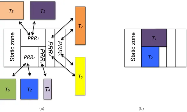
2.9 Reconfiguration by region -a- Placement possibilities of relocatable tasks on different P RR, -b- Example during runtime, T1executes on P RR1and T2 on P RR2 . . . 24
2.10 Microprocessor-based system controlling reconfigurable resources . . . 25
2.11 Stuffing and Classified Stuffing. The figure is taken from [1] . . . 29
2.12 Different algorithms to manage free space of the FPGA at runtime . . . . 32
2.13 -a- The placement of T2 creates the FPGA fragmentation and prevents T3 not to be placed -b- The placement of T2 creates a low FPGA fragmenta-tion and allows T3 to be placed . . . 33
2.14 -a-Feasible positions for T1, -b- feasible positions for T2 . . . 34
2.15 -a- Example of a 3D Silicon-in-Package (3DSiP), -b- Example of a 3D Package-On-Package (3DPoP) . . . 38
2.16 Staking techniques for 3DIC . . . 39
2.17 Virtex 7 - 2000T (figure taken from [2]) . . . 40
3.1 Assignment of T1, T2, T3 to two parallel processors . . . 45
3.2 Two possible types of communication between two communicating tasks . 47 3.3 Assignment of T1, T2, T3 to two parallel PRRs . . . 50
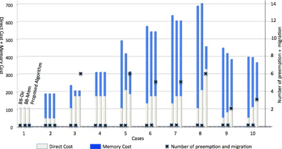
3.4 Comparison of different solutions in term of total communication cost and total number of preemptions and migrations . . . 52
3.5 VLS and MERs techniques . . . 55
3.6 Set of 8 dependent tasks . . . 60
3.7 Evolution of FPGA status and VLS at each insertion or extraction of task by using VLS-BCF strategy . . . 60
3.8 Evolution of FPGA status and VLS at each insertion or extraction of task by using VLS-BHF strategy . . . 61
3.9 Comparisons of direct communication cost for different scheduling and
placement techniques . . . 63
3.10 Comparisons of hotspots for different scheduling and placement techniques 63
4.1 3D Flextiles chip overview . . . 67
4.2 2D Heterogenous FPGA . . . 68
4.3 A set example comprising 4 tasks . . . 71
4.4 Different scenarios of task scheduling and placement for the task set in
Fig 4.3 . . . 73
4.5 -a- the placement of T2 prevents the placement of T3; -b- the placement
of T2 favors the placement of T3 . . . 74
4.6 Quick search method for finding all feasible regions Rk,i for the task Ti at
time t . . . 83
4.7 Scheduling and placement of tasks on 2D heterogenous FPGA . . . 86
4.8 Comparison of our method with others for 100 task sets executing on RR1
= {(36,34), (6,3), (8,8), (2,0), (8,8)} . . . 90
4.9 Comparison of our method with others for 100 task sets executing on RR2
= {(28,26), (6,3), (8,8), (2,0), (8,8)} . . . 91
4.10 Comparison of our method with others in terms of exploited computation
resources. . . 92
5.1 3D Homogeneous RSoC . . . 95
5.2 a - Classic model of the tasks graph ; b - The division of tasks in HW and
SW parts ; c- The proposed task graph model . . . 96
5.3 Task communication model for the 3D Homogeneous RSoC . . . 97
5.4 Placement solutions generated by the naive method and our proposed
method . . . 103
5.5 Comparison of the global communication cost generated by the algorithm
proposed in [3] and our 3DSTS algorithm for the case R = 100 . . . 106
5.6 -a- Example of a task graph model; -b- Each task has the possibility to be
run in SW or HW . . . 109
5.7 4 possible happening scenarios during a SW execution . . . 116
5.8 The scheduling scenario produced by our 3DHSSP stately . . . 118
5.9 Comparisons of the proposed algorithm to others in the case of
applica-tions with a high parallelism degree [5, 10] . . . 123
5.10 Simulator . . . 126
6.1 -a-example of three tasks with data dependencies; -b- Placing
communi-cating tasks far apart; -c- Placing communicommuni-cating tasks as close as possible132
List of Tables
2.1 Characteristics of three independent tasks T1, T2, T3 . . . 18
3.1 Characteristics of tasks. . . 45
3.2 Assignment of tasks onto 4 PRRs. NT : Total number of tasks, Dep: Total
number of dependencies, i.e the total number of edges in the task graph, E: the sum of execution cost of all the tasks, ExData : Total number of exchanged data between tasks, Sol: total number of possible solutions gen-erated by BB, BB-Dir: non-preemptive and non-migrating solution with the smallest direct communication cost (Dir), BB-Mem: non-preemptive and non-migrating solution with the smallest memory communication cost (Mem), Te: Total execution time, %Com: Gain in term of total commu-nication cost between our algorithm and BB, %Te: Gain in term of total execution time between our algorithm and BB, M: Total number of mi-grations due to our algorithm, P: Total number of preemptions due to our
algorithm . . . 51
3.3 Examples of implemented hardware tasks in [4] . . . 54
3.4 FPGA dimension and task characteristics . . . 63
4.1 Ti will be placed at R2,iin order to favor the placement of the next
recon-figurable task PL[2]. . . 85
4.2 Task set characteristic . . . 88
4.3 Comparisons of the overall execution time for different techniques . . . 88
5.1 Assignment of tasks to a 3D Homogeneous RSoC platform simplified
con-taining 4 processors and 4 PRRs. NT: Total numbers of task. (1): Overall
communication cost produced by the algorithm proposed in [3] . (2): Over-all communication cost produced by our 3DSTS algorithm. G: gain of our
algorithm compared to the one in [3] (%). . . 104
5.2 Task set characteristics with a low parallelism degree . . . 122
5.3 Comparisons of the proposed algorithm with others in the case of task
sets with a low parallelism degree [1-4] . . . 122
5.4 Application characteristic with a high parallelism degree . . . 122
Context
Les systèmes embarqués sont présents partout dans notre vie quotidienne. Nous ob-servons qu’ils sont intégrés dans une grande variété de produits : téléphone portable, machine à laver, voiture, avion, équipements médicaux, etc. Une grande majorité des microprocesseurs fabriqués de nos jours sont consacrés aux plate-formes de type systèmes embarqués. Un système embarqué peut contenir un ou plusieurs processeurs associés à d’autres composants comme les mémoires, les périphériques, les bus de communications et des composants spécifiques dédiés pour les applications cibles (comme le DSP, les ac-célérateurs, etc). L’évolution des technologies de fabrication conduit, d’année en année, à des composants de plus en plus petite taille et offrant des performances toujours plus importantes. Ces composants de systèmes embarqués peuvent donc être intégrés dans une seule puce, conduisant à ce qu’on appelle le système sur puce, ou encore "System On Chip" (SoC) en anglais.
Parallèlement à cette évolution des systèmes embarqués, les applications d’aujourd’hui sont de plus en plus complexes et gourmandes en puissance de calcul, en mémoire, en communication, etc. Les systèmes multiprocesseurs sur puce (MPSoC) sont des solutions qui peuvent répondre à cette complexité. Ces systèmes offrent non seulement une cer-taine flexibilité, grâce à la reprogrammation logicielle, mais aussi une grande capacité à exécuter en parallèle de nombreuses fonctionnalités. Ces solutions résultent de hautes performances pour le système mais ont l’inconvénient d’être statiques, i.e. elles ne per-mettent pas une adaptation et/ou des modifications après leur fabrication pour pouvoir s’adapter aux dynamismes d’applications.
Afin de répondre favorablement aux dynamismes des applications, les MPSoC doivent intégrer des ressources matérielles reconfigurables. Cela est rendu possible par l’intégra-tion de zones matérielles reconfigurables de type FPGA. Ces zones apportent la capacité d’adaptation et de reconfiguration au circuit tout en offrant des niveaux de performances très élevés. Au lieu de développer des circuits intégrés spécifiques à une application (ASIC), ce qui nécessite un délai de conception et un coût de production importants, le fait d’utiliser des zones reconfigurables, FPGA, donne la possibilité de mettre en oeuvre un nouveau système en reconfigurant les fonctionnalités adaptées aux nouvelles applica-tions. De plus, un des avantages de l’utilisation d’un FPGA au sein d’un MPSoC est la reconfiguration dynamique et partielle. Cette capacité permet de reconfigurer une partie
du FPGA en temps réel sans interrompre les autres parties en cours d’exécution. Le sys-tème combinant MPSoC et FPGA est appelé Reconfigurable Multiprocessor System On Chip (MPRSoC). Ce système disposé d’un support d’exécution logicielle et matérielle offert à la fois la haute performance, la flexibilité tout en limitant la surface globale du système.
L’évolution des systèmes sur puce ne cesse de s’accélérer, depuis environ une cinquantaine d’années. Aujourd’hui, cette évolution se poursuit avec l’apparition des technologies dites 3D, permettant la conception de systèmes sur puce en trois dimensions (ou 3DSoC). Comparer aux SoC planaires, cette technologie permet d’empiler verticalement des puces les unes sur les autres pour former un circuit en "stack". Il en résulte une augmentation des performances, une réduction de la longueur de communication en remplaçant la connexion horizontale par une courte connexion verticale, une réduction du coût de production en choisissant la technologie adaptée pour chaque puce et finalement une réduction de facteur de forme.
Les architectures considérées dans mon travail de thèse disposent de capacités de recon-figuration, il s’agit de circuits dit Reconfigurable System on Chip en trois dimensions (3DRSoC). Ces plate-formes sont constituées de deux couches qui sont verticalement connectées : la couche multiprocesseurs et la couche reconfigurable. Le fait d’empiler ces deux couches verticalement permet de conserver les caractéristiques du RSoC pla-naire tout en héritant des avantages offerts par la technologie 3D. En effet, en utilisant les connections verticales (de type microbumps ou TSVs), les communications entre la partie logicielle sur le MPSoC et la partie matérielle sur la zone reconfigurable peuvent être plus rapides et mieux assurées. Par conséquent, les architectures 3DRSoC sont une solution prometteuse qui répond mieux aux plus grandes variétés d’applications.
Motivations et Objectives
Le traitement d’une application est souvent découpé en tâches avec les dépendances entre elles. À cause de la complexité des applications, chaque tâche peut avoir différentes im-plémentations logicielles et/ou matérielles. Ces imim-plémentations donnent la possibilité, pour les tâches, d’être exécutées sur les différents composants de l’architecture. L’implé-mentation logicielle de la tâche (ou tâche logicielle) est une portion de code exécutable
sur un processeur. L’implémentation matérielle de la tâche (ou tâche matérielle) est une fonction synthétisée et configurable dans le FPGA. La gestion globale de l’architecture 3DRSoC nécessite un système d’exploitation adapté (Operating System OS) qui consiste à organiser l’ensemble des traitements d’une application sur cette plate-forme. Parallè-lement aux services de communication ou de gestion mémoire, cet OS doit égaParallè-lement fournir des méthodes d’ordonnancement pour la gestion et l’utilisation efficace des res-sources de calcul. Lors de l’exécution d’une application sur une architecture 3DRSoC, ces méthodes devront être capables de déterminer les ressources (le processeur ou la zone du FPGA) qui vont être utilisées par chaque tâche (dimension spatiale) à un instant donné (dimension temporelle) pour satisfaire les contraintes de coût de communication, de puissance de calcul, de consommation d’énergie, de temps d’exécution, etc. On parlera donc de l’ordonnancement spatio-temporel.
Pour les applications n’ayant pas de dynamisme, les décisions spatio-temporelles peuvent être prises hors-ligne, i.e. avant que l’application commence son exécution sur la plate-forme. Dans ce cas là, nous pouvons assurer l’optimalité des décisions. Cependant, pour les applications dynamiques dont le comportement dépend des événements extérieurs, les décisions spatio-temporelles pour les tâches doivent être prises "en-ligne", i.e. pendant l’exécution. Dans ce cas, le flot d’exécution des tâches, ainsi que le support d’exécution pour chaque tâche ne sont pas connus a priori. À cause de cette caractéristique "en-ligne", nous ne pouvons pas garantir que ces décisions donneront la solution optimale mais plutôt une solution qui est "proche de l’optimum".
Dans ce travail de thèse, notre objectif est de proposer des stratégies d’ordonnancement spatio-temporel pour les architectures de type 3DRSoC. Nos stratégies ciblent deux ob-jectifs : la minimisation du coût de communication entre les tâches et la minimisation du temps d’exécution global de l’application.
• Minimisation du coût de communication entre les tâches : Bien qu’il existe différents algorithmes d’ordonnancement spatio-temporel pour des RSoC planaire, la prise en compte de la troisième dimension de 3DRSoC rend le problème d’or-donnancement plus difficile à résoudre et ce problème se complexifie encore lorsque l’on considère les communications entre tâches. Comme les tâches peuvent être exécutées en logicielles et/ou en matérielles, elles peuvent communiquer de façon horizontale et/ou verticale. La communication entre deux tâches est liée aux temps
de transfert entre tâches et donc liée au nombre de données propagées lors de la communication. Plus la distance entre les tâches qui communiquent est grande, plus le coût de communication sera pénalisé. De plus, l’interconnexion de deux tâches affecte significativement le temps d’exécution global de l’application, la charge moyenne du réseau de communication, ainsi que la puissance et l’énergie consommées. Pour cette raison, il est très important de proposer des stratégies d’ordonnancement qui prennent en considération l’emplacement des tâches sur les trois dimensions afin de réduire au maximum le coût de communication entre les tâches.
• Minimisation du temps d’exécution global de l’application : Parce que les ressources du FPGA du 3DRSoC sont limitées, nous ne pouvons pas exécu-ter toutes les tâches de l’application en matérielle. Le support logiciel MPSoC du 3DRSoC est donc exploité pour offrir la possibilité d’exécuter certaines tâches en logicielle. Pendant l’exécution de l’application, les tâches sont anticipées sur une ressource de type processeur pour débuter leur traitement et libérées quand leur traitement est fini. À l’inverse d’une tâche logicielle dont l’exécution se fait sur un processeur, ces allocations et libérations des tâches matérielles peuvent causer la fragmentation du FPGA. Cela peut conduire à des situations indésirables où les futures tâches ne peuvent pas être placées sur le FPGA à cause de mauvais placements de tâches précédentes, même s’il y a suffisamment de zones libres. Ces tâches doivent attendre jusqu’au moment où il y aura des régions disponibles sur le FPGA pour les accueillir. Par conséquent, le temps d’exécution global de l’appli-cation sera augmenté et la performance globale du système sera pénalisée. Au lieu d’attendre que la tâche soit exécutée sur le FPGA, elle aurait pu être exécutée sur un des processeurs disponibles en vue d’anticiper leur traitement et ainsi s’achever plus rapidement. Nous nous intéressons aux stratégies d’ordonnancement spatio-temporel permettant de décider "en-ligne" des choix à prendre entre l’exécution logicielle et matérielle, à quel moment, sur quelle zone ou quel processeur pour minimiser le temps d’exécution global de l’application.
Contributions
Dans une architecture de type 3DRSoC, l’existence d’un FPGA est cruciale pour accélérer les traitements des tâches tout en maintenant une communication aisée et rapide avec les composants de la couche MPSoC. Rendre l’utilisation du FPGA plus efficace est extrêmement important pour atteindre la meilleure performance du 3DRSoC global. Dans ce travail, deux types d’architectures 3DRSoC sont considérés : le 3DRSoC homo-gène et 3DRSoC hétérohomo-gène. La différence de ces deux architectures vient de différents types de FPGA. Dans le 3DRSoC homogène, le FPGA est un modèle contenant des ressources reconfigurables homogènes tandis que dans la 3DRSoC hétérogène, le FPGA est un modèle contenant des ressources reconfigurables hétérogènes.
Notre contribution, dans un premier temps, consiste à étudier les stratégies d’ordonnan-cement spatio-temporel "en-ligne" pour un ensemble de tâches matérielles s’exécutant sur les différentes types de FPGA. Nous proposons :
• Pfair Extension for Reconfigurable Resource (Pfair-ERR) qui est une stra-tégie d’ordonnancement spatio-temporel pour un FPGA de type 2D Bloc Area. Dans ce type d’architecture, le FPGA contient plusieurs zones reconfigurables qui sont prédéfinies et figées. Ordonnancer les tâches sur ce type d’architecture est équivalent à un ordonnancement sur un système multiprocesseur. Pfair-ERR est une extension d’un algorithme dit Pfair qui est considéré comme optimal pour maximiser l’utilisation des processeurs dans un système multiprocesseurs. Le but de Pfair-ERR est de modifier le Pfair classique pour prendre en compte les dépen-dances entre les tâches et minimiser le coût de communication entre elles tout en maximisant l’utilisation des ressources du FPGA. Le travail sur Pfair-ERR a été publié dans [3].
• Vertex List Structure Best Communication Fit (VLS-BCF) qui est une stratégie d’ordonnancement spatio-temporel pour un FPGA de type 2D Free Area. Ce type d’architecture contient des blocs logiques reconfigurables, les zones recon-figurables ne sont pas prédéfinies a priori mais adaptative par rapport à la taille (ou les ressources) demandée par les tâches. VLS-BCF est basé sur un algorithme dit Vertex List Structure (VLS) ayant une faible complexité et une simple struc-ture de données pour la gestion des ressources de ce type de FPGA. L’objectif de
VLS-BCF est d’éviter de longues et couteuses communications, donc de réduire le coût de communication entre les tâches. Nous montrons ainsi que VLS-BCF permet de réduire également la probabilité de créer des points chauds sur le FPGA. Pour évaluer le VLS-BCF en termes de "points chauds", nous développons une solution dite VLS-BHF dont l’objective est d’ordonnancer et placer des tâches de façon à minimiser le nombre de "points chauds" tout en gardant un coût de communication faible. Ce travail a été publié dans [5].
• Spatio-Temporal Scheduling strategy for Heterogeneous FPGA (STSH) qui est une stratégie d’ordonnancement spatio-temporel pour un FPGA 2D hété-rogène. Ce type d’architecture contient non seulement des blocs logiques recon-figurables mais aussi d’autres blocs hétérogènes. Cette hétérogénéité impose des contraintes de placement strictes pour les tâches et nécessite une stratégie de cement différente. STSH prend en considération cette hétérogénéité dans son pla-cement. STSH combine la technique du "prefetching" avec deux autres facteurs : la priorité des tâches et le placement intelligent pour minimiser le temps d’exécution global de l’application. Le travail sur STSH a été publié dans [6].
Une fois que les stratégies d’ordonnancement sur les différentes architectures de FPGA ont été étudiées, nous étendons ces stratégies pour adresser le principal objectif de ces travaux qui a été de proposer des stratégies d’ordonnancement spatio-temporel "en-ligne" pour les architectures 3DRSoCs. Dans ce contexte, une tâche peut être exécutée matériellement et/ou logiciellement. Nous proposons les stratégies suivantes :
• 3D Spatio-Temporal Scheduling (3DSTS) qui consiste à prendre en considé-ration la troisième dimension pendant l’ordonnancement pour minimiser le coût de communication entre les tâches. La plate-forme considérée est une architecture 3DRSoC homogène dont la couche FPGA est de type 2D Bloc Area. 3DSTS évalue, pendant l’exécution de l’application, la nécessité de communiquer en face à face via les connections verticales pour trouver la meilleure instanciation possible des tâches (logicielle et matérielle) afin de minimiser le coût global de communication. Ce travail a été publié dans [7].
• 3D Hardware/Software with Software execution Prediction (3DHSSP) qui est une stratégie d’ordonnancement spatio-temporel pour une architecture 3DR-SoC hétérogène dont le FPGA est un FPGA 2D hétérogène. L’objectif de 3DHSSP est de décider et d’évaluer, pendant l’exécution de l’application, quelle tâche est exécutée en logiciel ou quelle tâche est exécutée en matériel afin de minimiser le temps d’exécution global de l’application. 3DHSSP évalue l’intérêt de continuer l’exécution logicielle d’une tâche en cours, ou d’annuler ce traitement pour com-mencer, à partir de l’état initial, l’exécution matérielle de cette tâche. Ce travail a été publié dans [8].
Introduction
Embedded systems are now present everywhere in our daily life and we observe their integration into a wide variety of products such as watches, cell phones, washing ma-chines, cars, planes, medical equipments, etc. To support the execution of large number of applications, these embedded systems contain one or more processors associated with other components such as memories, peripherals, communications bus and specific com-ponents (such as DSP, accelerators, etc.). This evolution is supported by the sophisticated IC fabrication technology which makes the components becoming smaller and smaller over time while offering even greater performance. These embedded system components can be integrated into a single chip, leading to a system called System On Chip (SoC). In parallel with the development of embedded systems, today’s applications are more and more complex and intensive in power computing, memory and communication, etc. To solve the application complexity, Multiprocessor system on chip (MPSoC) appears as an interesting solution by offering not only a certain flexibility through the software reprogramming, but also a great ability to run in parallel many tasks. Using such system results a high performance for the system but the drawback is its "static" nature, i.e. it does not allow adaptations and/or modifications after its manufacturing to follow dynamic applications.
To address favorably the dynamism of applications, MPSoC often embeds reconfigurable hardware resources. This incorporation is totally possible with the integration of hard-ware reconfigurable circuits as Field-programmable gate array (FPGA). These circuits
provide the ability to adapt and reconfigure themselves while offering very high perfor-mance levels. Instead of developing a specific integrated circuits (ASIC), which requires a significant design time and an important manufactory cost, using reconfigurable circuits as FPGA gives the possibility to implement a new system by reconfiguring the fea-tures adapted to new applications. In addition, one advantage of using a FPGA within a MPSoC is the dynamic and partial reconfiguration paradigm. This capacity allows to reconfigure a portion of logic blocks during runtime without interrupting the rest of the system. Therefore, the system can change its behavior during runtime according to its environment or external events. The system combining MPSoC and FPGA is called Multiprocessor Reconfigurable System On Chip (MPRSoC). This system disposing of a software and hardware execution support offers both the high performance and the flexibility while reducing the global area of the system.
1.1 3D multicore heterogeneous architecture context
The evolution of SoC has been increased for about fifty years. Today, it continues with the emergence of a so-called 3D technology, enabling the design of SoCs in three dimensions (3DSoC). Compare with planar SoCs, this 3D technology allows stacking layers vertically on top of each other to form a circuit said "in stack". The expected results are an increase in performance, a reduction of communication wires by replacing the horizontal connections with a short vertical connections and a form factor reduction. Moreover, the manufacturing cost is also reduced as each layer can be fabricated and optimized using their respective technology before assembling to form a circuit in stack.
T1 T2
T3
T4
Task graph application
3DRSoC architecture P1 P3 P4 P5 P6 P2 MPSo C laye r FPG A laye r V ert ica l l in k
The 3DSoCs having the reconfiguration capabilities is called 3D Reconfigurable SoCs (3DRSoCs). These platforms are composed of two layers that are vertically connected: the MPSoC layer and the FPGA layer. An example of a 3DRSoC is given in Fig1.1. Stacking these two layers allows to conserve the characteristics of planar RSoC while inheriting the benefits of 3D technology. By using the vertical connections, the communication between the software code running on the MPSoC layer and the hardware accelerators running on the FPGA layer can be faster and better ensured. Therefore, 3DRSoCs seems to be promising solutions that better addresses the largest varieties of applications.
1.2 Problematic, Motivations and Objectives
The treatment of an application is often divided into tasks with dependencies between them (for example in Fig1.1). Due to the complexity of applications, each task can have different software and/or hardware implementations. These implementations provide the opportunity for the tasks to be executed on the various components of the architecture. The software implementation of a task (or software task) is a piece of code executable on a processor. The hardware implementation of a task (or hardware task) is a synthesized and configurable function in the FPGA. From these task implementations, one of the challenge consists in managing the execution of all of them on the execution resources of the platform. One possible solution is then to embed an Operating System (OS) on the platform in order to organize the treatments of the application. The objective of an OS is to support several services, like the communication service, memory management, etc. and also the scheduling methods supporting an efficient management and use of computing resources. During the execution of an application on a 3DRSoC, the scheduling methods should be able to determine what resources (processor and/or FPGA area) are used by what task (spatial dimension) at what time (temporal dimension) in order to meet the communication cost constraints, the energy or power consumption budget, the overall execution time, etc. This problem, called spatio-temporal scheduling, is then more complex than the one of task scheduling for processor system.
For static applications, i.e. applications with a static execution flow of tasks, the spatio-temporal decisions can be taken offline, i.e. before the application starts running on the platform. In this case, we can ensure the optimality of these decisions. However,
for dynamic applications whose the behavior depends on external events, the spatio-temporal decisions for the tasks should be taken "online", i.e. during execution. In this case, the execution flow of tasks and the execution support for each task are not known a priori. Because of this "online" characteristic, we can not guarantee that these decisions will give the optimal solution. Therefore, online spatio-temporal scheduling strategies are proposed to find a "close to the optimum" solution.
The objective of my work consists in defining and evaluating a set of online spatio-temporal methods/strategies for 3DRSoCs. For this work, we propose to address several criteria, and to try to optimize them. The criteria and optimization are the following
• Minimizing the global communication cost of the application: in order to reduce the global communication cost of the application, the communication cost between tasks must be minimized. Although there exist different spatio-temporal scheduling algorithms for planar RSoC, taking into account the 3rd dimension of 3DRSoC makes the scheduling problem more difficult to solve and this problem is further complex when we consider the communication between tasks. As the tasks can be executed in software and/or hardware, they can communicate horizontally within a layer and/or vertically from a layer to another layer. The communications between tasks are linked to the time transfer between them and therefore related to the number of exchanged data during the communications. The more the com-munication distance between tasks is long, the more the comcom-munication cost will be penalized. Moreover, the interconnection of two tasks significantly affects the overall execution time of the application, the average load of the communication network and the power and energy consumed. For this reason, it is very impor-tant to propose scheduling strategies that take into consideration the placement of tasks on the three dimensions in order to minimize the communication cost between tasks, thus minimize the global communication cost of the application.
• Minimizing the overall execution of the application running: because the resources of the FPGA in a 3DRSoC are limited, it cannot accommodate all the tasks of the application at the same time. In this context, the MPSoC layer in 3DR-SoC is used as a software support which offers the possibility of performing certain tasks as software. Thus, during the execution of the application, the execution of tasks can be anticipated on processors. Contrary to a software task whose execution
is done in a processor, the allocations and deallocations of hardware tasks at run-time can cause the FPGA fragmentation. This can lead to undesirable situations where future tasks can not be placed on the FPGA due to the bad placements of previous tasks, even there would be enough space. These tasks must be delayed until there will be available regions on the FPGA to accommodate them. There-fore, the overall execution time of the application will be increased and the overall performance of the system will be penalized. Instead of waiting for the task to be performed on the FPGA, the task could be executed on an available processor to anticipate their treatment and thus be completed sooner in time. In this case, a spatio-temporal strategy is necessary to support anticipation decision of software tasks and to be able to confirm or not the software anticipation when needed in order to minimize the overall execution time of the application.
1.3 Contributions
In 3DRSoC architectures as the one defined in Fig1.1, the existence of the FPGA layer is crucial to accelerate the task processing while maintaining an easy and fast commu-nication with the components of the MPSoC layer. Compare with software tasks, the management of hardware tasks on the FPGA layer is more complex and should be taken more carefully into account. On one hand, because the interconnection between hardware tasks consumes logical elements and routing signals. On the other hand, because a bad placement of a hardware task can prevent the placement of future tasks, thus penalize the overall execution time of the application. Making the use of FPGA more efficient is extremely important to achieve the best performance of the global 3DRSoC system. Therefore, before tackling spatio-temporal scheduling strategies for the 3D architectures, it is very important to study the spatio-temporal scheduling strategies for the FPGA layer.
In this work, two types of 3DRSoC architectures are considered: the 3D Homogeneous RSoC and the 3D Heterogeneous RSoC. The difference of these two 3DRSoCs comes from the FPGA layer architectures. In the 3D Homogeneous RSoC, the FPGA is a homoge-neous reconfigurable resources model while in the 3D Heterogehomoge-neous RSoC, the FPGA is a heterogeneous reconfigurable resources model. The details of these two 3DRSoCs will be given later in this thesis.
To address the problematic of spatio-temporal task scheduling on the 3D Homogeneous RSoC and the 3D Heterogeneous, we organize our work into four steps. The first two steps consist in analyzing and proposing spatio-temporal scheduling strategies for the FPGA layer of these two 3DRSoCs:
• Step 1: we propose spatio-temporal scheduling strategies for hardware tasks exe-cuted in the homogeneous reconfigurable resources. These strategies aim at reduc-ing the communication cost between tasks so that the global communication cost is minimized.
• Step 2: we address the heterogeneity of the reconfigurable resources. This hetero-geneity imposes a stricter placement for hardware tasks, thus requires a differ-ent spatio-temporal strategy. We propose a strategy supporting this heterogeneity which aims at minimizing the overall execution time of the application.
Then, the step 1 and step 2 are served for addressing our main contributions which are in the step 3 and the step 4:
• Step 3: we extend the strategies proposed for homogeneous reconfigurable resources in step 1 to take into account the 3rd dimension of the 3D Homogeneous RSoC. Our strategy considers the 3rd dimension during the task scheduling in order to minimize the global communication cost of the application.
• Step 4: we address the spatio-temporal scheduling strategy for the 3D Heteroge-neous RSoC. Our strategy exploits our previous work developed for the heteroge-neous reconfigurable resources in step 2 and proposes to anticipate the software execution of a task if needed.
For all these proposed strategies, we have developed simulation models. A simulation tool has been developed and enables us to produce results. An hardware implementation of a complete platform is not part of this work but it is currently in progress, and will enable us to include our strategies in the scheduling service of an Operating System.
1.4 Thesis Organization
According to the objectives of our work and the different steps to address the global problematic, we organize this thesis in following chapters:
• Chapter 2 presents a background on the real-time system and gives the state-of-the-art overview of scheduling methods for MPSoC system, for different types of FPGA. The 3D technology and some scheduling methods on 3D platforms are presented as well.
• Chapter 3, addressing the step 1 of the contribution part, presents two online spatio-temporal scheduling strategies: the Pfair Extension for Reconfigurable Resource (Pfair-ERR) algorithm dealing with reducing the communication cost between tasks in a 2D bloc area FPGA and the Vertex List Structure Best Communica-tion Fit (VLS-BCF) also aiming at reducing the communicaCommunica-tion between tasks but in a 2D free area FPGA. The results show that by limiting long and costly communications between tasks, the global communication cost of the application is significantly reduced.
• Chapter 4, addressing the step 2 of the contribution part, presents the online Spatio-Temporal Scheduling strategy for Heterogeneous FPGA (STSH) which deals with minimizing the overall execution time of an application running on this platform. STSH integrates prefetching technique while considering the priority of tasks and the placement decision to avoid conflicts between tasks. The results show that STSH leads to a significant reduction of the overall execution time compared to some non-prefetching and other existing prefetching methods. It also leads to a better FPGA resource utilization compared to others.
• Chapter 5, addressing the step 3 and 4 of the contribution part, presents the main contributions of this thesis. In this chapter, two online spatio-temporal scheduling strategies are introduced: the 3D Spatio-Temporal Scheduling (3DSTS) for the 3D homogeneous RSoC and the 3D Hardware/Software with Software execution Prediction (3DHSSP) algorithm for the 3D Heterogeneous RSoC. 3DSTS consists in considering the 3rd dimension during the scheduling and placement of tasks in order to minimize the global communication cost. 3DHSSP dealing with reducing
the overall execution time of applications, exploits the presence of processors in the MPSoC layer in order to anticipate a SW execution of a task when needed. • Chapter 6 concludes this thesis and gives some perspectives
Background and Related Works
As previously mentioned, the objective of this work concerns the definition of run-time task scheduling and placement for 3DRSoCs. However, in order to tackle the 3D sys-tems, it is also necessary to analyze the influence of this issue on 2D systems such as: multiprocessor and reconfiguration architecture systems.
This chapter presents the background and the state-of-the art of the task scheduling and placement problem. It is composed of four sections. Section 2.1 presents real-time systems and discusses some existing scheduling methods for multiprocessor architecture systems. Section 2.2 introduces the reconfigurable architectures and presents a survey of existing techniques for task scheduling and placement for reconfigurable architecture systems. Section2.3 presents the 3D technologies and related works for the 3D system. Finally, we conclude this chapter with our proposed approaches.
2.1 Real-time Systems
Real-time systems can be classified as two different categories: hard real-time systems or soft real-time systems. In hard real-time systems, all temporal constraints must be strictly respected. Any missing deadline will lead to catastrophic consequences. Hard real-time systems are used in military applications, space missions or automotive systems. Some examples of hard real-time systems are: fly-by-wire controllers for airplanes, monitoring systems for nuclear reactors, car navigation, robotics, etc.
In soft real-time systems, some temporal mistakes can be tolerated. They will decrease the quality of service, but they will not affect the correctness of the system. Web services, video conferencing, cell phone call are examples of soft real-time systems.
For these two types of real-time systems, the task scheduling is an important issue and large number of studies have been published in the literature. When the system archi-tecture becomes more and more complex by including large number of heterogeneous processing cores, solving the task scheduling issue is critical and needs new schedul-ing strategies. Furthermore, when the system is submitted to large environment events, runtime decisions are necessary to support the dynamism of the application.
2.1.1 Offline and Online Scheduling
The scheduling service plays a very important role of an operating system. For a simple core processor, which executes just one task at a time, the scheduling has to determine the execution time of the tasks and manages the execution resource. For multiprocessors architectures, the scheduling is more complex by also determining the allocation of tasks on different execution resources.
Real-time task scheduling determines the order in which various tasks are selected for an execution on a set of resources. The real-time aspect consists in ensuring that each task respects its deadline execution time. To ensure this constraint, two different schedul-ing approaches are available for real-time systems: offline and online schedulschedul-ing. Offline scheduling is applicable for applications where the execution flow of task set is known a priori. Thus, tasks are executed in a fixed order and this order is determined offline, i.e. before the system gets started. Offline scheduling is usually performed to find the optimal solution of tasks.
Contrary to the offline scheduling, the execution flow is not known in advance for online scheduling. All scheduling decisions are made on the fly without any knowledge of future arriving tasks. Online scheduling selects tasks to execute by analysis of their priorities. It is more flexible than offline scheduling since it can be used for the cases where the sequence of tasks dynamically changes at run-time. In almost cases, online scheduling algorithms try to produce an "approximate" solution, but can not guarantee the optimal solution.
2.1.2 Static and Dynamic scheduling
Most scheduling algorithms are priority-based and consist in determining the task pri-orities in different ways. There are two priority-based algorithms: static-priority and dynamic-priority.
Static-priority means there is an unique priority associated to each task. This priority is determined before the system runs and it will stay unchanged during the system execution. Among static-priority algorithms, Rate Monotonic (RM) [9] is known as the optimal algorithm. RM assigns priority according to the period, thus a task with a shorter period has a higher priority and will be executed first.
In dynamic-priority, the priority of a task is not fixed and can be changed during the execution. Earliest deadline first (EDF) [10], Least Completion Time (LCT) and Least-Laxity First (LLF) [11] are some examples of dynamic priority scheduling algorithms. In the context of embedded systems, the dynamism requirement leads the designer to embed an operating system which supports dynamic scheduling. Static scheduling is often not implemented due to the inefficient processor usage.
2.1.3 Type of tasks
Before presenting different types of tasks, we introduce here some basic task character-istics which would be useful for the understanding of this work.
• Task instance: each new execution of a task is called a task instance or a job. A task can be executed one or several times, i.e. a task can have one or several instances. • Relative and absolute deadline: Absolute deadline is the time point at which the job should be completed. Relative deadline is the time length between the arrival time and the absolute deadline.
2.1.3.1 Periodic, Aperiodic and Sporadic tasks
Depending on the real-time application, tasks can be executed repetitively (in the case of reading the ambient temperature at regular intervals for example) or non-repetitive. A task can be classified into three following categories:
Ti
0 = Ai t
First instance Second instance
Ti Ei
Pi = Di
Ti (a) periodic and preemptive task
0 t
Tj
Relative deadline = Dj Absolute deadline = Aj + Dj
Aj Sj
(b) aperiodic and non-preemptive
Figure 2.1: -a-Example of a periodic and preemptive task; -b- Example of an aperiodic and non-preemptive task
• Periodic: a periodic task Ti is characterized by (Ai, Ei, Pi, Di) with Ai as the release time (or arrival time), i.e. the time the task is ready to be scheduled, Ei
as the worst case execution time (the maximum amount of time the task required to execute), Pi as the period of the task, Di as a relative deadline (Di = Pi for
almost cases). A job (or an instance) of the task is repeated indefinitely and the time length between two activations of successive instances is called "period". A job is released at the beginning of its period and must complete execution before the end of its period.
• Aperiodic: an aperiodic task Ti is characterized by (Ai, Ei, Di) with Ai as the arrival time, Ei as the worst case execution time, and Di as the absolute deadline. An aperiodic task must run at least once and it is not necessary to be repeated. In offline or static scheduling, the arrival time of a job is known before execution. In online scheduling and dynamic scheduling, the arrival time of a job is not known before execution, it will be computed on the fly. For an aperiodic task, the response time of a job is defined by the subtraction of the completion time and the arrival time of this job. In some cases, another parameter Sj, representing the time point that a task starts its execution, is also used to characterize the aperiodic task. • Sporadic: sporadic tasks are a particular case of a periodic task. These are tasks
repeated with a minimum period. A sporadic task Tiis characterized by: the arrival
time Ai, the worst case execution time Ei, a relative deadline Diand the minimum time M Ti between two successive jobs.
Fig2.1(a)shows an example of a periodic and preemptive task Tiwith Ti=(Ai,Ei,Pi,Di).
shown in the Fig2.1(b). The definition of a preemptive and non-preemptive task will be given just below.
2.1.3.2 Preemptive and Non-Preemptive tasks
Tasks are also distinguished by two types of execution: preemptive and non-preemptive execution. In order to respect the real-time constraints, it is generally necessary to use preemptive tasks, i.e. a task that can be interrupted by higher priority tasks and resumed to finish its execution later. However, preemptive tasks create overhead needed to switch between tasks. Non-preemptive tasks do not permit the preemption before the end of the job execution. This type of execution is easier to implement than preemptive execu-tion one. Non-preemptive tasks guarantee exclusive access to shared resources and data which eliminates both the need for synchronization and its associated overhead [12]. For soft real-time applications, using non-preemptive tasks are usually more efficient than preemptive scheduling.
As previously mentioned, the context of embedded systems needs adaptative execution of tasks, and non-preemptive execution is generally not implemented due to the difficulty to rapidly react when a new event occurs.
2.1.3.3 Migrable and Non-Migrable tasks
Some advanced real-time applications require more than one processor to complete set of tasks efficiently and successfully. A migrable task is the term used when a suspended instance of a task may be resumed on different processors. Otherwise, every instance of non-migrable tasks always executes on the same processor.
The migration concept enables more flexibility for the execution, but this flexibility generates time overhead to move the context of task from one processor to another. When the processor cores are heterogeneous, migration of tasks is yet more complex because the task context must be transformed in order to be able to resume the task execution after the migration.
2.1.3.4 Dependent and Independent tasks
For almost applications, tasks are dependent and need to share data between them. Precedence constraints and data dependencies are often modeled by a directed acyclic graph (DAG). Formally, a DAG consists of several nodes (tasks) that can be executed on any available processors. An edge signifies that data produced by one task is used by another one. The number on an edge represents the cost of the communication, and can be the amount of exchanged data between two tasks. We call Tj the predecessor of Ti if Ti needs data from Tj to be executed. A task can have one or more predecessors and it is ready to execute when all of its predecessors complete their execution and produce their data. Fig2.2 shows an example of a DAG comprising 5 tasks with the amount of exchanged data between tasks.
T1 5698 T2 T3 1475 T4 4931 T5 268 9251
Figure 2.2: Example of a DAG task graph
2.1.4 Real-time Scheduling on Multiprocessors System
One of the main factors to measure the performance of multiprocessor systems is to analyze the scheduling of tasks in order to verify if the different processors are used as efficiently as possible at each time. Almost task scheduling algorithms consist in distribut-ing a set of tasks among the processors to achieve the desired objective as: minimizdistribut-ing the schedule length, minimizing the communication cost between tasks or maximizing the processor utilization, etc. In this section, we introduce different multiprocessor systems and talking about the importance of scheduling in such systems. Existing scheduling algorithms are then presented and discussed.
2.1.4.1 Multiprocessors definition
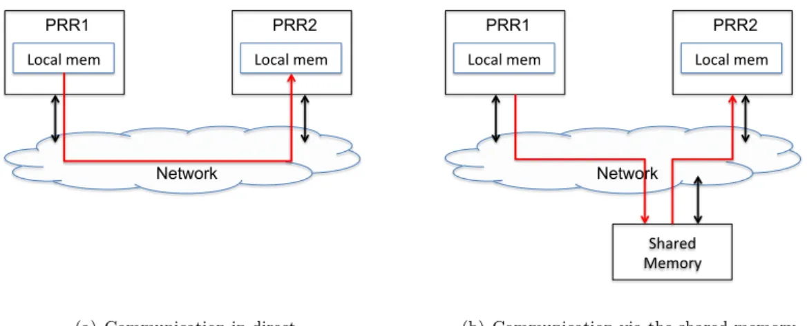
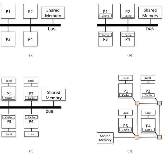
A multiprocessor system is composed of many processors communicating with each other by an interconnect network. This network can be a communication bus or a network on chip (NoC). The simplest multiprocessors are described as in the Fig 2.3(a) where processors do not have any cache memory or local memory. Every read/write operation must use the communication bus to access to the shared memory. In such system, the bandwidth of the bus is limited as a processor must wait until the bus is idle in order to perform the read/write operation. A more evolved multiprocessor system has a cache added to each processor, this solution enables to reduce bus traffic toward the memory
(Fig 2.3(b)). Another possibility is the system where each processor proceeds a cache
memory and a local (private) memory (Fig 2.3(c)). In that case, every local variables, local data, constants, etc, are placed in the local memory. The shared memory is then only used for writable shared variables which will greatly reduce the contention for the bus. Fig2.3(d) shows a multiprocessor interconnected by a NoC.
Considering the memory accesses, a multiprocessor system can be differentiated by two types: Uniform Memory Access (UMA) or Non Uniform Memory Access(NUMA). In UMA, each processor needs the same time to read a word from the shared memory. NUMA does not support this property, and the access time from/to the memory depends on the memory location relative to the processor.
2.1.4.2 Partitioning and Global Scheduling
Scheduling algorithms for multiprocessor systems are generally divided into two cat-egories: partitioning and global scheduling. In partitioning scheduling, a task is only scheduled on a predefined processor and it cannot be moved to another processor during runtime. With partitioning method, the migration of tasks between different processors is not allowed. For all the cases, the scheduling scenario is well-studied before the sys-tem gets started and optimal partitioning of tasks is defined if it exists. This method reduces the complexity of the scheduler, but it can be inefficient in some cases where tasks must be migrated in order to respect several constraints of the system as: deadline, communication cost, temperature, energy, etc.
P1 P2 P3 P4 Shared Memory bus (a) P1 P2 P3 P4 Shared Memory Cache Cache Cache Cache bus (b) P1 P2 P3 P4 Shared Memory Cache Cache Cache Cache Local Local Local Local bus (c) P1 P2 P3 P4 Shared Memory Cache Cache Cache Cache Local Local Local Local (d)
Figure 2.3: Multiprocessor systems with different data-communication infrastructures
In global scheduling, tasks are ordered by the scheduler during run-time. Tasks which are ready to be scheduled are stored in a single list (or queue) regarding the task priorities. Then, the highest priority task is selected by the scheduler to be executed on any avail-able processor. Global scheduling allows task migration in order to satisfy the required constraints.
A semi-partitioned scheduling algorithm has been also proposed in [13], this algorithm limits the number of processors which can support a task execution. Thus, the penalties associated to task migration are reduced and the implementation of the system is less complex.
2.1.4.3 Performance parameters of scheduling algorithms
Many parameters can be used to evaluate the performances of scheduling algorithms. The basic parameters are following:
• Processor utilization: the performance of a scheduling algorithm is measured by the processor utilization, i.e. how all the processors are effectively used. The processor utilization is calculated by:
U =
n
X
i=1
Ei/Pi
where Ei is the worst case execution time of Ti and Pi is the period of Ti (Pi is
assumed to be equal to the relative deadlines Di). A set of tasks is said schedulable in a uniprocessor system when and only when U ≤ 1. It is said schedulable in a multiprocessor system of Np processors when and only when U ≤ Np.
• Effectiveness: effectiveness of a scheduling algorithm can be measured by any factor for example: communication cost, overall execution time, energy, etc.
• Number of preemptions and migrations: it measures the number of preemptions of the tasks and the number of migrations that the tasks performed.
• Response time: the time duration between the time point when a task is ready to be executed and the time point when it finishes its execution.
• Deadline missed: the number of tasks which miss their deadline. This parameter is only used for soft real-time system, for hard real-time this case should not appear. • Complexity: scheduling algorithm complexity is about how fast the algorithm per-forms. If a scheduling algorithm is complex, it may need a huge computation time and lead to delays in real-time systems.
2.1.4.4 Scheduling of independent tasks on multiprocessors
EDF [10] is known to be the optimal scheduling algorithm for independent and preemp-tive tasks in uniprocessor system. Fig 2.4 shows the EDF scheduling of 3 independent tasks T1, T2, T3 in uniprocessor system. The characteristics of these tasks are described in the table 2.1. All the deadlines are met and the processor utilization is 100%.
Task Ai Ei Di
T1 0 1 6
T2 0 2 4
T3 0 4 12
Table 2.1: Characteristics of three independent tasks T1, T2, T3
0 1 2 3 4 5 6 7 8 9 10 T1 T2 T3 11 12 t
Figure 2.4: Earliest deadline first (EDF) scheduling in uniprocessor system
However, EDF is not optimal on multiprocessors since some deadlines may be not re-spected if EDF is used. Let’s consider another example of scheduling 3 periodic tasks T1=(0,2,4,4), T2=(0,2,4,4) and T3=(0,7,8,8) on two processors using EDF. T1 and T2 will
execute on processor 1 and processor 2 because they have a higher priority than T3. As
a result, T3 can only start executing from time 2 and will miss its deadline. But if T1 and T2 execute on the same processor (one after the other) and T3 executes on another
processor. Every task will meet their deadline.
Another dynamic scheduling algorithm, called Least-Laxity First (LLF) [11], is based on task laxity to define scheduling priority. The laxity of a task is defined by the subtrac-tion of the deadline and the remaining execusubtrac-tion time of this task. LLF is optimal for independent and preemptive tasks whose the relative deadlines are less or equal to their period. But LLF is still not optimal in a multiprocessor system.
Pfair [14] has been proved optimal for real-time scheduling of periodic tasks on a mul-tiprocessor system. However, the migration and preemption costs are not taken into account in Pfair. In the worst case, a task may be migrated or preempted each time it is scheduled. For a real-time system, these can occur to significant delay and it can lead to degrade the performance of the system. To limit this problem, some other works based on Pfair are proposed to reduce at maximum the number of preemptions and migrations. Some of them are Generalized Deadline partitioned fair (DP-Fair) [15] or BFair [16].
A survey on real-time task scheduling is done in [17]. Fig2.5shows different scheduling algorithms with different parameters considered. However, almost of them consider that tasks are independent in the nature, i.e. no communication exists between tasks.
Figure 2.5: Real-time task scheduling algorithms
2.1.4.5 Scheduling dependent tasks on multiprocessors
Scheduling of dependent tasks onto a set of homogeneous processors in order to minimize some performance measures has been quite studied for a long time. One of important performance measure is communication delays. Reducing the communication delays leads to not only the overall schedule length reduction but also the energy consumption re-duction. If two communicating tasks Ti and Tj are executed on different processors, they will incur a communication cost penalty depending on the distance between two pro-cessors and the amount of exchanged data between two tasks. Otherwise, if Ti and Tj are executed on the same processor, the communication cost can be estimated to value zero. Smit et al [18] present a mapping algorithm to map an application task-graph at run-time. Communicating tasks are placed as closed as possible in order to save the en-ergy consumption. Similarly, Singh et al [19] propose a number of communication-aware run-time mapping heuristics for the efficient mapping of multiple applications onto an 8 x 8 NoC-based MPSoC platform. Their technique tries to map the communicating tasks on the same processing resource and also the tasks of an application close to each other in order to reduce the communication overhead. Their proposed heuristics lead to reduction in the total execution time, energy consumption, average channel load and latency.
Two others important performance measures are the total duration of the schedule and the running time execution of the algorithm. There is usually a trade-off between these two performance measures: a proposed algorithm searching for the optimal solution in-curs normally a high time running. Using Branch-and-Bound technique or integer linear programming (ILP) solver can find the optimal solution, but they need a huge com-putation time. Thus, many heuristics are proposed to quickly find an close-to-optimal solution in a polynomial-time. Some of them are based on list scheduling technique. The idea is to assign priorities to tasks and place the tasks in descending order of priorities in a list. The highest priority task is executed first. If some tasks have the same pri-ority, several methods are used to decide in which order the tasks are executed. Some given priority functions are EDF, dynamic critical path, as late as possible, etc. Some of them based their algorithms on Tabu Search [20], Simulated Annealing [21] or ant colony optimization [22] technique in order to optimize the execution time.
Most of previous algorithms target offline scheduling. In online scheduling, if the entire execution flow is not known in advance, the scheduling decision must be done on the fly by using dynamic-priority of tasks. In this context, previous methods as ILP solver, Branch-and-Bound or other mentioned algorithms cannot be applied.
2.2 Task Scheduling And Placement for Reconfigurable
Ar-chitecture
2.2.1 Reconfigurable Architecture
A configurable logic circuit is a circuit whose logic function can be configured. This type of circuit is made from basic logic elements and a set of them can be used to ensure a specific function. Reconfiguration concept means that it is possible to change the configuration if needed.
A circuit is said dynamically reconfigurable when it is possible to change its configuration during the execution of an application on the system. A circuit is said to be dynamically and partially reconfigurable when it is possible to change during the operation of the sys-tem and when the configuration can address a portion of the circuit, without interfering other running parts.
2.2.1.1 FPGA circuits
Several types of architectures exist and allow reconfiguration. The reconfiguration can be applied for operators of a processor or for hardware accelerators of a System-on-Chip (SoC) or in FPGA. Among them, FPGA is known as a very wised used reconfigurable architecture allowing a high configuration flexibility.
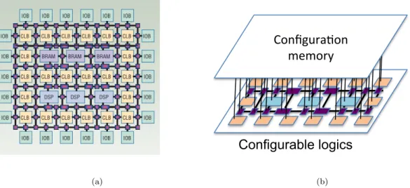
FPGA is a configurable logic device consisting of an array of configurable logic blocks (CLBs), programmable interconnects and programmable input/output blocks (IOBs). The CLB block is composed of Lookup Tables (LUTs), multiplexers (MUXs), Flip-Flops and registers. CLBs are connected together as well as to the programmable IOBs through programmable interconnects. Currently, FPGA can contain also Digital Signal Process-ing (DSP) blocks which have high-level functionality embedded into the silicon, and embedded memories (BRAMs). All these blocks are configurable to perform the required functionalities. Fig 2.6(a) represents a FPGA internal structure based on the Xilinx architecture style [23] (a)
Configura)on
memory
Configurable logics
(b)Figure 2.6: -a-Example of a Xilinx architecture style, -b-Two layers representation of a reconfigurable architecture
FPGA can be represented as a circuit having two layers (Fig2.6(b)): one layer for the ar-chitecture whose functionalities are configurable and another layer for the configuration memory. This memory stores all the configuration information and the FPGA is config-ured by charging the bitstream in this memory. A bitstream is a sequence of bits that are stored in the external memory of the FPGA as Compact Flash or internal memory

![Figure 2.11: Stuffing and Classified Stuffing. The figure is taken from [1]](https://thumb-eu.123doks.com/thumbv2/123doknet/14590598.730089/50.893.224.711.601.1010/figure-stuffing-classified-stuffing-figure-taken.webp)