HAL Id: hal-01770233
https://hal-amu.archives-ouvertes.fr/hal-01770233
Submitted on 20 Jun 2018
HAL is a multi-disciplinary open access
archive for the deposit and dissemination of
sci-entific research documents, whether they are
pub-lished or not. The documents may come from
teaching and research institutions in France or
abroad, or from public or private research centers.
L’archive ouverte pluridisciplinaire HAL, est
destinée au dépôt et à la diffusion de documents
scientifiques de niveau recherche, publiés ou non,
émanant des établissements d’enseignement et de
recherche français ou étrangers, des laboratoires
publics ou privés.
Modular Modelling of an Embedded Mobile CPU-GPU
Chip for Feature Estimation
Oussama Djedidi, Mohand Arab Djeziri, Nacer M’Sirdi, Aziz Naamane
To cite this version:
Oussama Djedidi, Mohand Arab Djeziri, Nacer M’Sirdi, Aziz Naamane.
Modular Modelling of
an Embedded Mobile CPU-GPU Chip for Feature Estimation.
14th International Conference
on Informatics in Control, Automation and Robotics, Jul 2017, Madrid, Spain.
pp.338-345,
�10.5220/0006470803380345�. �hal-01770233�
Oussama Djedidi, Mohand Arab Djeziri, Nacer K. M’Sirdi and Aziz Naamene
Laboratoire des Sciences de l’Information et des Syst`emes (LSIS), Aix-Marseille University, Marseille, France
Keywords: Embedded Chips Central Processing Units, Graphics Processing Units, Modelling Simulation.
Abstract: This paper deals with the modelling of a CPU-GPU chip embedded in an Android phone. The model is used for the estimation of variables that characterise the operating state of System on Chip (SoC). The proposed model is built to demonstrate the causal relationships between the variables, through its interconnected structure of subsystems. This structure allows the extension of other components or the easy exchange of subsystems in the case of a change in components or operating mode. The model developed here requires no additional instrumentation—other than the one present on the phone—which facilitates its implementation. It is used for the estimation of the state of the system and can also be used for monitoring and behaviour prediction. The model is validated and the results are promising for further implementation.
1
INTRODUCTION
Modelling of Central Processing Units (CPU) and Graphics Processing Units (GPU) chips is done for a multitude of purposes. The first and foremost is to en-sure performance reliability which can be done either by selecting the algorithms to be implemented and predicting their performance (M’Sirdi et al., 2016; Williams et al., 2009; Meng and Skadron, 2011), or running background programs in parallel that are able to predict the performance output of some compo-nents (Ardalani et al., 2015), or even by thoroughly studying the component itself (Kim et al., 2012a). However, in this work, we are more interested in the monitoring of the operating state of the chip. Hence, we focus our modelling on the physical variables i.e. frequency, voltage, power consumption, and temper-atures in the SoC.
Reducing power consumption and improving bat-tery life in mobile phones is a very active research area. Thus, several models estimating the power con-sumption of embedded CPU-GPU chips were devel-oped. For instance, Zhang et al. propose a model called ”PowerBooter” to the estimate power con-sumption of a smartphone through its battery sen-sors (Zhang et al., 2010). Another study used sys-tem calls to estimate the power consumptions (Pathak et al., 2011), while others used polynomial and re-gression models in a series of works to estimate the power consumption of smartphone components
in-cluding the CPU and the GPU (Minyong Kim et al., 2012; Kim et al., 2012b; Kim and Chung, 2013; Kim et al., 2015). These studies offer simple modelling techniques and also show a clear dependence between frequency and power consumption.
Furthermore, several other notable studies focused on the power consumption of just the GPU. For in-stance, Leng et al. estimate the power consumption, in a discrete GPU, as a sum of three components, the dynamic power (power consumed by the GPU while running computations), the leakage power (es-sentially linked to transistor leakage currents in the architecture of the chip) and idle power (assumed con-stant) (Leng et al., 2013). Additionally, in their work, Adhinarayanan et al. present a GPU power estima-tor based on multiple regression techniques, that uses performance counters and temperature to deliver ac-curate power estimation at runtime (Adhinarayanan et al., 2016).
As Temperature is an important variable in the functioning and life cycle of CPU and GPU, several models were developed in the literature to study its profile and behaviour, such as the model developed by Hong et al., which is a switched system with two first order models, one for the rise in temperature and the second for cooling. The time constants of these mod-els were identified experimentally, and static gains are presented as a function of the maximum temperature of the system, power consumption, and memory in-tensity (Hong and Kim, 2010).
338
Djedidi, O., Djeziri, M., M’Sirdi, N. and Naamane, A.
Modular Modelling of an Embedded Mobile CPU-GPU Chip for Feature Estimation. DOI: 10.5220/0006470803380345
Amongst the works mentioned above, there are fine grained models of the CPU-GPU chips, like the model proposed by Kim et al. which models perfor-mance as a function of of memory warps and models temperature as a function of memory intensity (Kim et al., 2012a). Nonetheless, such models use variables which are neither measurable nor accessible to read, such as the memory intensity for instance or are spe-cific to certain GPU brands like the warps.
Moreover, because of the complexity of the sys-tem and physical phenomena, inputs of the models constructed by machine learning are not the subject of a formal proof of the interaction between the inputs and estimated outputs. The choice of model inputs is often the result of observations and experimental tests in various operating conditions. These models are of-ten built to give developers feedback on on perfor-mance, and power consumption, which will be used for program optimisation. The temperature estima-tion is, generally, used to set temperature thresholds for thermal throttling to keep the component out of harm’s way.
The model proposed in this paper is built in a modular structure, and is composed of a set of inter-connected subsystems, where the control components (subsystems for frequency and voltage) are clearly distinguished from the operating ones (power and temperature), allowing thus the model to adapt to changes in the system operating modes. The sub-systems are inspired by those presented in the stud-ies above and the algorithms given by manufacturers. The developed model is then used to estimate a set of variables characterising the operating state of the CPU-GPU system. Our main goal behind the devel-opment of this model is to use its generated estimation to monitor the state of the chip.
This paper is organised as follows. The targeted system is described is Section 2. In Section 3, we de-scribe the data aquisition, then the modelling method and the models of each subsystem are detailed in Sec-tion 4. In SecSec-tion 5, the model is validated by compar-ing the real and estimated outputs, then, the results are discussed. Finally, a conclusion is given in Section 6.
2
TARGETED SYSTEM
DESCRIPTION
The electronic devices market proposes differ-ent CPU and GPU architectures. Each fam-ily of architecture comes with its own advantages and—naturally—complexities. One of the main goals of this work is to construct a general dynamic model for embedded CPU-GPU chips. Thus, for testing and
undertaking experimental validation, the choice of a System on Chip (SoC) to be studied is firstly based on the software it runs.
For this study, we settled on an AndroidTMphone. AndroidTM phones are very popular, and with its pro-gramming framework, aoolications are effortlessly transferable to other devices. Moreover, Android is built on top of the popular open source operating sys-tem (OS) Linux. The availability of the code for this OS makes some of the needed parameters accessible for reading. Furthermore, the system’s terminal, via Android Debugging Bridge (ADB), gives access to all system files, some of which are used for variables reading.
The smartphone we used in this study runs on AndroidTM Marshmallow 6.0, and is equipped with a SoC harbouring a quad-core processor with variable frequencies—through frequency and voltage scal-ing—ranging between 300 MHz–2.45 GHz. It also sports an OpenGLTM ES 3.0 capable GPU with fre-quencies ranging between 200 MHz–578 MHz. The SoC also contains the systems 2 GB RAM.
3
VARIABLES AND DATA
ACQUISITION
To analyse and model the dynamics of the CPU-GPU chip, one must initially recover the relevant readings characterising the operating state of the system. For our modelling purposes, the needed readings are the loads of both the CPU and the GPU, the working fre-quencies, temperatures of the cores and other com-ponents, the voltage of each core and the power de-livered by the battery. All of these variables–except for the temperature–have very fast variations. There-fore, the quality of the results depends directly on the chosen sampling period. Hence, we choose the min-imum period necessary to follow the changes of the fast changing variable: the frequency. Frequency is evaluated by by frequency Governor (see paragraph 4.1). Hence, the minimum period for this program to reevaluate the load and change of the frequency accordingly was set as sampling period (in this case study, Ts= 20 ms).
Since we do not wish to hinder the normal be-haviour of the system while reading the variables, we have written a lightweight application for data acqui-sition. However, during periods of high loads, the sys-tem will give priority to the user interface and syssys-tem operations over background services (like our app), which sometimes leads to the scheduling of our ap-plication excecution being pushed back, and thus the chosen sampling period Tsbeing not respected. Fig. 1
Modular Modelling of an Embedded Mobile CPU-GPU Chip for Feature Estimation
shows the evolution of the sampling periods during a reading experience where some sampling values are well beyond the chosen period Ts and even reaching
tens of seconds.
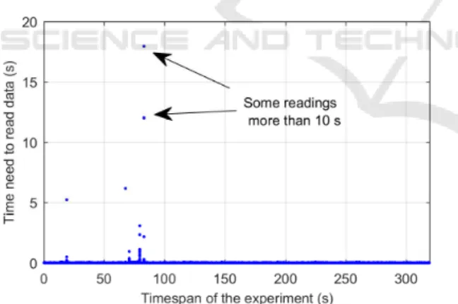
Figure 1: Sampling time variation over time. The second difficulty in reading the variables is related to the management of instruction queues by the OS. Again, during periods of high the CPU loads, we came to notice that reading time—the time differ-ence between the start of the reading process and its end—is sometimes very long, even reaching seconds (See Fig. 2), leading to the conclusion that the reading was interrupted. This renders the values taken during the said reading false (unsynchronized data, measure-ments delays and missing data).
Figure 2: Reading time evolution and variation over time. These two problems of data acquisition are taken into account and the data acquired during long sam-ple times or interrupted readings will be automatically deleted from the database used in the next section for learning and model assessment.
4
SYSTEM MODELLING
The CPU-GPU chip is a complex system with vari-able structure, whose dynamics are nonlinear and not
continuous. Hence, a gradual approach and a modu-lar structure are adopted for its modelling as shown in Fig. 3. This modular approach provides for a gradual analysis and modelling each of the subsystems and account for the variable structure of the system. It also allows easy integration of subsystems in case of any changes. Fig. 3 shows a global vision of the in-terconnected and gradual modelling approach. In the following paragraphs, each of the subsystems will be detailed. ⋮ Governor Load1 Load2 Load3 Loadn ⋮ f1 f2 f3 fn Thermal Regulator On/Off On/Off On/Off On/Off Power Model Voltage Model Thermal Model GPU Governor LoadGPU fGPU V1, V2, V3… Vn T1, T2, T3… Tn Pconsumed MOR X
Figure 3: Diagram of the proposed model of the CPU-GPU system.
4.1
The Frequency Scaling Governor
Frequency scaling is carried out via Governors. On the studied system, several frequency governors exist. These governors calculate the frequency according to usage needs as well as several other factors (speed, power consumption). The governor we are modelling in this work is the interactive governor. However, thanks to the modular structure of the model, any governor can replace the one considered in this case study.
The interactive governor increases and decreases the frequency of each core as a function of the load and specific timers. When the CPU is back from the idle state, the governor starts a countdown timer with a predefined timer rate value at the end of which, if the load exceeds a given value (go hispeed load), the governor calculates a new frequency for which the load will be equal or closest to target load value.
The governor also takes into account sudden heavy loads by directly scaling up the frequency to
hispeed freq if the current frequency is below it for
better reactiveness and to avoid unexpected CPU bot-tlenecks and sluggish performance. In addition, if the frequency of a core is greater or equal to hispeed freq, the core must stay on the same frequency at least a pe-riod of above hispeed delay, before scaling up, and a period of min sample time (or sampling down factor if the current frequency is the maximum frequency) before scaling down. The last time constant, noted
timer slack, is an additional period of time that the
core has to wait before shutting down if the load is equal to zero. The governor modelling algorithm is given in Fig. 4 and Fig. 5. This model is engineered
from the original source code available in the code de-posits of the manufacturer of the studied smartphone (Samsung, 2016).
procedure INTERACTIVE(Load, Time, currentFrequency)
define above hispeed delay, hispeed freq,
go hispeed load, min sample time, target load,
sampling down factor,timer slack,timer rate
if Initialisation= 0 then currentHiSpeedTimer← 0 currentTimers← 0 currentDownTimers← 0 currentTimersSlack← 0 oldTime← Time; Initialisation← 1 else
currentHiSpeedTimer← currentHiSpeedTimer + (Time − oldTime)
currentTimers← currentTimers + (Time − oldTime) currentDownTimers ← currentDownTimers + (Time − oldTime)
currentTimersSlack ← currentTimersSlack + (Time − oldTime)
end if
if (currentTimers≥timer rate) then
if (Load≥go hispeed load) then
if (currentFrequency < hispeed freq ∧
ChooseFreq(Load, currentFrequency) <hispeed freq) then newFrequency←hispeed freq
else if (ChooseFreq(Load, currentFrequency) >
hispeed freq)∧ (currentHiSpeedTimer ≥above hispeed delay) then
newFrequency ←
ChooseFreq(Load, currentFrequency)
else if (ChooseFreq(Load, currentFrequency) <
currentFrequency)∧ (currentDownTimers ≥ min sample time) then
newFrequency ←
ChooseFreq(Load, currentFrequency)
else if (Load = 0) ∧ (currentTimersSlack ≥
timer slack) then
newFrequency← 0 end if currentHiSpeedTimer← 0 currentDownTimers← 0 end if else newFrequency← currentFrequency end if return newFrequency end procedure
Figure 4: The Interactive Governor algorithm (I—The gen-eral algorithm).
4.2
Voltage Model
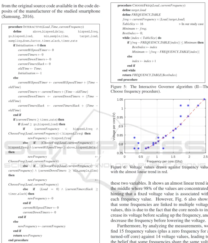
Recovered readings show that, like frequency, volt-age is discrete and varies in a set of well-defined val-ues. Voltage readings are plotted against the frequen-cies, in Fig. 6, in order to see the relationship between
procedure CHOOSEFREQ(Load, currentFrequency)
define target load define FREQUENCY TABLE
f req= currentFrequency× (Load/target load)
TableSize← 16 ⊲ In our study case
Minimum← f req; BestIndex← 0;
while(index < TableSize) do
if| f req − FREQUENCY TABLE(index)| ≤ Minimum then
BestIndex← index
Minimum← | f req − FREQUENCY TABLE(index)| else
index← index + 1 end if
end while
return FREQUENCY TABLE(BestIndex)
end procedure
Figure 5: The Interactive Governor algorithm (II—The Choose frequency procedure).
0 0.5 1 1.5 2 2.5
Frequency per core (Ghz) 0.75 0.8 0.85 0.9 0.95 1 1.05
Voltage per core (V)
Figure 6: Voltage values drawn against frequency value with the almost linear trend in red.
these two variables. It shows an almost linear trend in the middle where 98% of the values are concentrated, hinting that a fixed voltage value is associated with each frequency value. However, Fig. 6 also shows that some frequencies are linked to multiple voltage values, this is due to the fact that the core needs to in-crease its voltage before scaling up the frequency, and decrease the frequency before lowering the voltage.
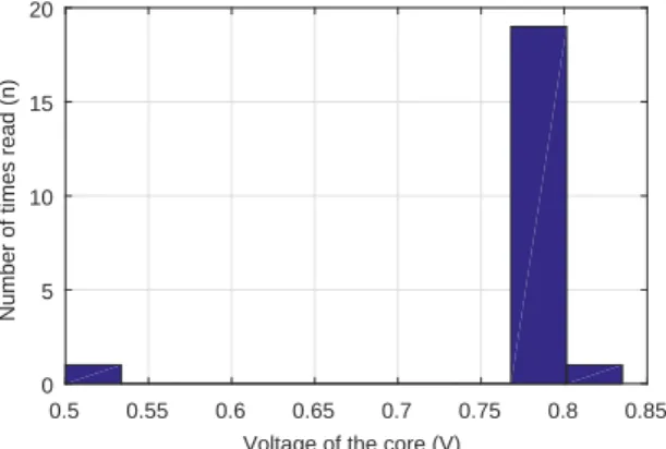
Furthermore, by analyzing the measurements, we find 15 frequency values (plus a zero frequency for a turned-off core) against 14 voltage values, leading to the belief that some frequencies share the same volt-age value. Thus, to better investigate the relationship between the frequencies and voltages, a histogram of voltage values for each frequency is constructed. Fig. 7 shows the histogram of voltage values for f= 300 MHz indicating that the voltage associated with this frequency value is clearly V300MHz= 0.775V. All other voltage values are obtained following the same fashion.
Modular Modelling of an Embedded Mobile CPU-GPU Chip for Feature Estimation
0.5 0.55 0.6 0.65 0.7 0.75 0.8 0.85 Voltage of the core (V)
0 5 10 15 20
Number of times read (n)
Figure 7: Histogram of voltage values for f= 300 MHz.
4.3
The Thermal Regulator
Thermal management is a very important task, espe-cially during boot and system startup periods where the temperature can become excessively high. The al-gorithms used during startup are generally fixed and not accessible to the programmer. However, in the user space, SoC manufacturers generally implement programmable algorithms for programmers to use. In the smartphone we are studying, the SoC manu-facturer implemented three types of regulators from which the programmer can choose to manage the tem-perature of the SoC. The implemented regulators are Proportional Integral Derivative (PID), Single Step, and finally, the one used by the manufacturer of the studied smartphone a Monitor.
This algorithm samples the temperature every
sampling ms. If the temperature of the core is higher
than a predefined thresholds, the core is shutdown. Once the temperature of the said core drops below
thresholds clr, it can be turned on again.
4.4
Power Model
In the relevant literature, some works, such as the one presented by Wang et al., use battery measurements to estimate the power consumed by applications (Wang et al., 2013). Others track kernel queries to determine power consumption (Pathak et al., 2011). Other tech-niques, like the one presented in (Kim et al., 2012b; Kim and Chung, 2013; Kim et al., 2015) involve the construction of polynomial models to estimate the power consumption as a function of the frequency and of the load. In this case study, we use battery readings. However, the obtained value of the current supplied by the battery is a constant, and the value of voltage varies in a set of fixed values which results in staircase-like power output signal, and makes any convergence of polynomial and auto-regressive
mod-els (ARX, ARMA, ...) impossible. Additionally, in order to minimise the influence of the other compo-nents of the smartphone, all communication and sec-ondary peripherals (WiFi, screen, cameras ...) were disabled and assumed to consume a static constant amount of power in that state.
Before starting the modelling process, it is neces-sary to determine the model inputs. In the case of the CPU, the power consumption is often given by the re-lation (Adam Kerin, 2013) :
PCPU= f×V2×C (1)
where f denotes the frequency, V the voltage and C the electric charge stored in the CPU, which is rel-atively constant. Thus, the CPU power becomes a function of the frequency and voltage. It was shown in the previous subsection that the voltage is itself a function of frequency. For the GPU, voltage mea-surements are not available in this case study, thus its frequency is used as input of the model (Kim et al., 2015). The last input is the Memory Occupation Rate (MOR)—the ratio of the occupied memory to the full memory—which will help include the memory power consumption in the model, since it is a part of the SoC. The model developed to estimate power consump-tion is a neural network with two layers. A hidden layer whose activation function is a sigmoid, and con-taining 8 neurons, and an output layer concon-taining a single neuron with a linear transfer function.
4.5
Temperature Model
Heat transfer and temperature modelling have been studied quite extensively in the relevant literature. However, in this work, we will not focus on the me-chanics of heat generation and transfer since its aim is to estimate temperature for monitoring and diagnosis purposes. Thus we focused our attention on finding variables affecting it i.e. correlations.
Temperature dynamics are different from those of the other studied variables; for one it does not range in a specific set of values. Furthermore, it does not de-pend only on the inputs, but also on its own previous values. It is directly correlated with the frequency of the CPU and the GPU. However, as shown in (Hong and Kim, 2010), we note that the correlation in the measurements between the recorded temperature and power consumption is imperceptible, which was con-firmed by our own results. Therefore, the considered inputs of the model of the SoC temperature are the frequencies and the MOR.
The temperature readings (Fig. 11) show two main trends for which we should account. The first is the rise (warming) and fall (cooling) of temperature
occurring over relatively long periods of time, and the second is the high-frequency small temperature changes. To better represent these dynamics, we chose to use an autoregressive–moving-average (AR-MAX) model. ARMAX models use the regression of inputs and previous outputs, along with the moving average to simulate or predict the current output:
y(k) = P1y(k− 1) + ... + Pny(k− n)
+ Q1u(k− 1) + ... + Qmu(k− m)
+ e(k) + H1e(k− 1) + ... + Hre(k− r) (2)
Equation (2) is the linear difference equation of an ARMAX(n, m, r) (orders of the model), with y(k) being the output to compute, u the exogenous (X) variable or system input, and e is the moving av-erage (MA) variable ((Fung et al., 2003)). In the case of this work, temperature TSoC is the output
y(k) to be estimated, and the system input is u(k) = [ f1, ..., f4, fGPU, MOR]. The parameters P, Q, and H
are constants evaluated by iterative search algorithms.
5
EXPERIMENTAL AND MODEL
VALIDATION
The experimental results presented in this section are obtained through the application then compared with estimations made by the model. The evolutions of the measured frequencies of one core, and the frequencies estimated by the model are given in Fig. 8. The plots are nearly identical, with a slight delay at the instants of frequency changes. The maximum delay recorded τf = 0.2 s. This result validates the frequency model.
3474 3476 3478 3480 3482 3484 Time (s) 0 0.5 1 1.5 2 2.5 Frequency f (GHz) fReading fSimulated
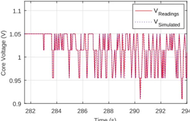
Figure 8: Frequency model estimations vs system readings. Fig. 9 shows the evolution of the measured volt-age of one core, compared to the estimated one. As for frequencies, the plots are again nearly identical, with a slight delay at the instants of voltage changes. The maximum delay recordedτV= 0.22s. Thus, the
voltage model is, also, validated.
282 284 286 288 290 292 294 Time (s) 0.9 0.95 1 1.05 1.1 Core Voltage (V) VReadings VSimulated
Figure 9: Voltage model estimations vs system readings. The measured power delivered by the battery compared to the estimated power by the neural net-work model are given in Fig. 10. This result shows the good accuracy of the model during the slow vari-ations and static phase. However, there is also notice-able noise during the phase of rapid changes, espe-cially between t= 50 s and t = 60 s. The Mean Abso-lute Error (MAE) recorded is 0.0083 W over 2× 10⁵ samples, with a maximum error of 6.60%, while the Mean Squared Error (MSE) is 2.3896× 10⁻⁴. Thus, the power model is validated.
0 10 20 30 40 50 60 70 80 Time (s) 1.5 1.6 1.7 1.8 1.9 Power (W) PSimulated PReadings
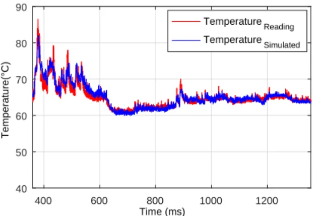
Figure 10: Power model estimations vs system readings. Fig. 11 shows the evolution of the estimated temperature compared with the measured tempera-ture. The model accurately follows the dynamics of the measured temperature during temperature change (heating and cooling), and also during phases with weak temperature changes. Fig. 11 also shows that the model takes into account the initial conditions of temperature. It has an MAE of 0.9947◦C, with a one time maximum of 8.14%, and an MSE of 1.8584. Hence, the temperature model is also validated.
Modular Modelling of an Embedded Mobile CPU-GPU Chip for Feature Estimation
400 600 800 1000 1200 Time (ms) 40 50 60 70 80 90 Temperature(°C) Temperature Reading Temperature Simulated
Figure 11: Temperature model estimations vs system read-ings.
6
CONCLUSION
A data acquisition and estimation systems have been developed for a CPU-GPU embedded chip. Measure-ments are acquired on the fly for operational state es-timation.
The estimation model developed is validated ex-perimentally. The parameter and variable estimation is structured as an interconnected system with vari-able structure. The modularity of the estimation sys-tem is easily adaptable to changes in the syssys-tem struc-ture and its operation modes.
In future works, the next step after developing the model is to use it to monitor the operating state and drifts in characteristics of the chip.
ACKNOWLEDGEMENT
This paper is a part of the MMCD project supported and funded by the BPI, to whom we address our thanks along with the FUI 19 project partners : IN-RIA, IRTS, and Nolam ES.
REFERENCES
Adam Kerin (2013). Power vs. Performance Management of the CPU.
Adhinarayanan, V., Subramaniam, B., and Feng, W.-c. (2016). Online Power Estimation of Graphics Pro-cessing Units. In IEEE/ACM International
Sympo-sium on Cluster, Cloud and Grid Computing (CC-Grid), number May, Colombia.
Ardalani, N., Lestourgeon, C., Sankaralingam, K., and Zhu, X. (2015). Cross-architecture performance prediction (XAPP) using CPU code to predict GPU performance.
Proceedings of the 48th International Symposium on Microarchitecture - MICRO-48, pages 725–737.
Fung, E. H., Wong, Y., Ho, H., and Mignolet, M. P. (2003). Modelling and prediction of machining errors using ARMAX and NARMAX structures. Applied
Mathe-matical Modelling, 27(8):611–627.
Hong, S. and Kim, H. (2010). An integrated GPU power and performance model. In ACM SIGARCH
Com-puter Architecture News, volume 38 of{ISCA} ’10,
page 280, New York, NY, USA. ACM.
Kim, H., Vuduc, R., Baghsorkhi, S., Choi, J., and Hwu, W.-m. (2012a). Performance Analysis and Tun-ing for General Purpose Graphics ProcessTun-ing Units (GPGPU), volume 7. Morgan & Claypool publishers.
Kim, M. and Chung, S. W. (2013). Accurate GPU power estimation for mobile device power profiling. Digest
of Technical Papers - IEEE International Conference on Consumer Electronics, pages 183–184.
Kim, M., Kong, J., and Chung, S. W. (2012b). En-hancing online power estimation accuracy for smart-phones. IEEE Transactions on Consumer Electronics, 58(2):333–339.
Kim, Y. G., Kim, M., Kim, J. M., Sung, M., and Chung, S. W. (2015). A novel GPU power model for ac-curate smartphone power breakdown. ETRI Journal, 37(1):157–164.
Leng, J., Hetherington, T., ElTantawy, A., Gilani, S., Kim, N. S., Aamodt, T. M., and Reddi, V. J. (2013). GPUWattch: Enabling Energy Optimizations in GPG-PUs. Proceedings of the 40th Annual International
Symposium on Computer Architecture - ISCA ’13,
41:487.
Meng, J. and Skadron, K. (2011). A performance study for iterative stencil loops on GPUs with ghost zone opti-mizations. International Journal of Parallel
Program-ming, 39(1):115–142.
Minyong Kim, Joonho Kong, and Sung Woo Chung (2012). An online power estimation technique for multi-core smartphones with advanced display components. In
2012 IEEE International Conference on Consumer Electronics (ICCE), pages 666–667. IEEE.
M’Sirdi, S., Godard, W., and Pantel, M. (2016). A Multi-Core Interference-Aware Schedulability Test for IMA Systems, as a Guide for SW/HW Integration. In 8th
European Congress on Embedded Real Time Software and Systems (ERTS 2016), TOULOUSE, France.
Pathak, A., Hu, Y. C., Zhang, M., Bahl, P., and Wang, Y.-M. (2011). Fine-Grained Power Modeling for Smart-phones Using System Call Tracing. Proceedings of
the sixth conference on Computer systems EuroSys 11,
page 153.
Samsung (2016). Samsung Opensource Release Center. Wang, C., Yan, F., Guo, Y., and Chen, X. (2013). Power
estimation for mobile applications with profile-driven battery traces. Int Symp on Low Power Electronics
and Design, pages 120–125.
Williams, S., Waterman, A., and Patterson, D. (2009). Roofline: An Insight Visual Performance Model for Multicore Architectures. Communications of the ACM, 52(4):65.
Zhang, L., Tiwana, B., Qian, Z., Wang, Z., Dick, R. P., Mao, Z. M., and Yang, L. (2010). Accurate on-line power estimation and automatic battery behav-ior based power model generation for smartphones. In IEEE/ACM/IFIP int conf Hardware/software
code-sign and system synthesis - CODES/ISSS ’10, page
105, New York, New York, USA. ACM Press.
Modular Modelling of an Embedded Mobile CPU-GPU Chip for Feature Estimation