Synthesizing invariants : a constraint programming approach based on zonotopic abstraction

HAL Id: tel-02925914

https://tel.archives-ouvertes.fr/tel-02925914

Submitted on 31 Aug 2020

HAL is a multi-disciplinary open access

archive for the deposit and dissemination of

sci-entific research documents, whether they are

pub-lished or not. The documents may come from

teaching and research institutions in France or

L’archive ouverte pluridisciplinaire HAL, est

destinée au dépôt et à la diffusion de documents

scientifiques de niveau recherche, publiés ou non,

émanant des établissements d’enseignement et de

recherche français ou étrangers, des laboratoires

Synthesizing invariants : a constraint programming

approach based on zonotopic abstraction

Bibek Kabi

To cite this version:

Bibek Kabi. Synthesizing invariants : a constraint programming approach based on zonotopic

ab-straction. Computer science. Institut Polytechnique de Paris, 2020. English. �NNT : 2020IPPAX017�.

�tel-02925914�

NNT

:

2020IPP

AX017

Synthesizing invariants: a constraint

programming approach based on

zonotopic abstraction

Th `ese de doctorat de l’Institut Polytechnique de Paris pr ´epar ´ee `a l’ ´Ecole Polytechnique

´

Ecole doctorale n◦_{626 ´Ecole doctorale de l’Institut Polytechnique de Paris (ED IP}

Paris)

Sp ´ecialit ´e de doctorat : Informatique Th `ese pr ´esent ´ee et soutenue `a Paris, France, le 24 Juin 2020, par

B

IBEK

KABI

Composition du Jury :

Laurent Fribourg

Directeur de Recherche, ENS Paris-Saclay (LSV) Pr ´esident

Charlotte Truchet

Maˆıtre de Conf ´erences, Universit ´e de Nantes (LINA) Rapportrice

Michel Rueher

Professeur Em ´erite, Universit ´e Cote d’Azur Rapporteur

Khalil Ghorbal

Charg ´e de Recherche, INRIA Rennes Examinateur

Antoine Min ´e

Professeur, Sorbone Universit ´e (LIP6) Examinateur

Eric Goubault

Professeur, ´Ecole polytechnique (LIX)) Examinateur

Sylvie Putot

Professeur, ´Ecole polytechnique (LIX) Directrice de th `ese

Eric Goubault

Résumé

Les systèmes dynamiques sont des modèles mathématiques pour décrire l’évo-lution temporelle de l’état d’un système. Il y a deux classes de systèmes dynamiques pertinentes à cette thèse : les systèmes discrets et les systèmes continus. Dans les systèmes dynamiques discrets (ou les programmes informa-tiques classiques), l’état évolue avec un pas de temps discrets. Dans les systèmes dynamiques continus, l’état du système est fonction du temps continu, et son évolution caractérisée par des équations différentielles. Étant donné que ces systèmes peuvent prendre des décisions critiques, il est important de pou-voir vérifier des propriétés garantissant leur sûreté. Par exemple, sur un programme, l’absence de débordement arithmétique.

Dans cette thèse, nous développons un cadre pour la vérification auto-matique des propriétés de sûreté des programmes. Un élément clé de cette vérification est la preuve de propriétés invariantes. Nous développons ici un algorithme pour synthétiser des invariants inductifs (des propriétés vraies pour l’état initial, qui sont stables dans l’évolution des états du programme, donc sont toujours vraies par récurrence) pour des programmes numériques. L’interprétation abstraite (IA) est une approche traditionnelle pour la recherche d’invariants inductifs des programmes numériques. L’IA interprète les ins-tructions du programme dans un domaine abstrait (par exemple intervalles, octogones, polyèdres, zonotopes), domaine qui est choisi en fonction des propriétés à prouver. Un invariant inductif peut être calculé comme limite possiblement infinie des itérées d’une fonctionnelle croissante. L’analyse peut recourir aux opérateurs d’élargissement pour forcer la convergence, au détriment de la précision. Si l’invariant n’est pas prouvé, une solution standard est de remplacer le domaine par un nouveau domaine abstrait davantage susceptible de représenter précisément l’invariant.

La programmation par contraintes (PPC) est une approche alternative pour synthétiser des invariants, traduisant un programme en contraintes, et les résolvant en utilisant des solveurs de contraintes. Les contraintes peuvent opé-rer sur des domaines soit discrets, soit continus. La programmation classique par contraintes continues est basée sur un domaine d’intervalle, mais peut approximer une forme invariante complexe par une collection d’éléments abs-traits. Une approche existante combine IA et PPC, raffinant de façon itérative, par découpage et contraction, une collection d’éléments abstraits, jusqu’à obte-nir un invariant inductif. Celle-ci a été initialement présentée en combinaison avec intervalles et octogones. La nouveauté de notre travail est d’étendre ce cadre au domaine abstrait des zonotopes, un domaine sous-polyédrique qui présente un bon compromis en terme de précision et de coût. Cette extension demande de définir de nouveaux opérateurs sur les zonotopes, pour permettre

Résumé

le découpage et la contraction, ainsi que d’adapter l’algorithme générique. Nous introduisons notamment un nouvel algorithme de découpage de zonotopes basé sur un pavage par sous-zonotopes et parallélotopes. Nous proposons également des alternatives à certains opérateurs existants sur les zonotopes, mieux adaptés que les existants à la méthode. Nous avons implé-menté ces opérations dans la bibliothèque APRON et avons testé l’approche sur des programmes présentant des invariants complexes, éventuellement non convexes. Les résultats démontrent un bon compromis par rapport à l’utilisation de domaines simples, comme les intervalles et les octogones, ou d’un domaine plus couteux comme les polyèdres. Enfin, nous discutons de l’extension de l’approche pour trouver des ensembles d’invariants positifs pour des systèmes dynamiques continus.

Abstract

Dynamical systems are mathematical models for describing temporal evolution of the state of a system. There are two classes of dynamical systems relevant to this thesis : discrete and continuous. In discrete dynamical systems (or classical computer programs), the state evolves in discrete time steps, as described by difference equations. In continuous dynamical systems, the state of the system is a function of continuous time, characterized by differential equations. When we analyse the behaviour of a dynamical system, we usually want to make sure that it satisfies a safety property expressing that nothing bad happens. An example of a safety property of programs is the absence of arithmetic overflows. In this thesis, we design a framework related to the automatic verification of the safety properties of programs. Proving that a program satisfies a safety property of interest involves an invariance argument.

We develop an algorithm for inferring invariants more precisely inductive invariants (properties which hold during the initial state, remains stable under the program evolution, and hence hold always due to induction) for numerical programs. A traditional approach for finding inductive invariants in programs is abstract interpretation (AI) that interprets the states of a program in an abstract domain (intervals, polyhedra, octagon, zonotopes) of choice. This choice is made based on the property of interest to be inferred. Using the AI framework, inductive invariant can be computed as limits of iterations of functions. However, for abstract domains which feature infinite increasing chain, for instance, interval, these computations may fail to converge. Then, the classical solution would be to withdraw that particular domain and in its place redesign a new abstract domain which can represent the shape of the invariant. One may also use convergence techniques like widening to enforce convergence, but this may come at the cost of precision. Another approach called constraint programming (CP), can be used to find invariants by translating a program into constraints and solving them by using constraint solvers. Constraints in CP primarily operate on domains that are either discrete or continuous.

Classical continuous constraint programming corresponds to interval domain and can approximate a complex shape invariant by a set of boxes, for instance, upto a precision criterion. An existing framework combines AI and continuous CP inspired by iterative refinement, splitting and tightening a collection of abstract elements. This was initially presented in combination with simple underlying abstract elements, boxes and octagons. The novelty of our work is to extend this framework by using zonotopes, a sub-polyhedric domain that shows a good compromise between cost and precision. However, zonotopes are not closed under intersection, and we had to extend the existing framework, in addition to designing new operations on zonotopes.

Abstract

We introduce a novel splitting algorithm based on tiling zonotopes by sub-zonotopes and parallelotopes. We also propose few alternative operators to the existing ones for a better efficiency of the method. We implemented these operations on top of the APRON library, and tested it on programs with non-linear loops that present complex, possibly non-convex, invariants. We present some results demonstrating the interest of this splitting-based algorithm to synthesize invariants on such programs. This algorithm also shows a good compromise by its use in combination with zonotopes as regards to its use with both simpler domains such as boxes and octagons, and more expressive domains like polyhedra. Finally, we discuss the extension of the approach to infer positive invariant sets for dynamical systems.

Contents

I Introduction and State of the Art

1 Introduction 14

1.1 Motivation . . . 14

1.1.1 Safety properties of programs . . . 14

1.2 Our contribution . . . 20

1.3 Thesis outline . . . 21

2 Abstract Interpretation 22 2.1 Abstract interpretation . . . 22

2.2 Notations and Definitions . . . 23

2.3 Numerical abstract domains . . . 31

2.3.1 Non-Relational Abstract Domain . . . 32

2.3.2 Relational Abstract Domains . . . 33

Polyhedras . . . 33

Ellipsoids . . . 35

2.3.3 Weakly-relational abstract domains . . . 35

Octagons . . . 37

Template polyhedra . . . 38

Affine sets or zonotopes . . . 38

Parallelotope abstract domains . . . 45

2.3.4 Combining abstract domains . . . 46

2.3.5 Support libraries . . . 47

2.3.6 Abstract interpretation tools . . . 47

3 Constraint Programming 49 3.1 From AI to CP . . . 49

3.2 Constraint programming . . . 50

Abstract

3.2.2 Splitting . . . 52

3.2.3 A continuous solver . . . 52

4 Interactions between Abstract Interpretation and Constraint Programming 54 4.1 Are we introducing AI ideas into CP or CP into AI? . . . 54

4.2 Refinement-based inductive invariant inference . . . 55

4.2.1 Concrete semantics. . . 55 4.2.2 Target invariant. . . 56 4.2.3 Abstract semantics. . . 56 4.3 Search algorithm. . . 58 4.3.1 Coverage . . . 60 4.3.2 Tightening . . . 62 4.3.3 Splitting . . . 62 4.3.4 Size . . . 62 4.3.5 Failure . . . 62 4.3.6 Data structure. . . 63 4.4 Related work . . . 64

4.4.1 CP using SAT/SMT solvers . . . 64

4.4.2 SAT-based model checking . . . 65

4.4.3 Combined AI and CP approaches . . . 65

4.4.4 Learning loop invariants . . . 66

4.4.5 Eigen vectors as invariants . . . 67

II Invariants of discrete systems

5.2 Inclusion test . . . 71 5.3 Intersection test . . . 74 5.4 Meet . . . 74 5.5 Size . . . 81 5.6 Volume of a zonotope. . . 82 5.7 Coverage metric . . . 83

5.7.1 Test for benign. . . 85

5.8 Splitting . . . 86

5.8.1 Splitting with overlap . . . 86

5.8.2 Effect of partitioning on splitting . . . 88

5.8.3 Splitting zonotopes by tiling . . . 91

Concepts and Definitions . . . 91

A survey on zonotopal tilings . . . 94

De Bruijn grids school . . . 94

Hyperplane arrangement-matroid theory school . 97 Is zonotopal tiling a vertex enumeration problem? . . . 98

Our tiling algorithm . . . 101

Hyperplane arrangements and zonotopes . . . . 101

Enumerating sign vectors . . . 102

Notions whose sequel is the tiling algorithm . . . 102

6 Implementation and experiments on programs 118

6.1 Implementation . . . 118

6.1.1 Apron . . . 118

6.1.2 Taylor1+ . . . 118

6.1.3 Our contribution with respect to implementation . . . . 119

6.2 Experiments . . . 119

6.3 Conclusion . . . 130

III Invariants of Continuous Systems

7.2 The CP algorithm revisited . . . 136

7.3 Taylor model approximation of flow map . . . 148

7.3.1 Picard iteration . . . 152

Operations on Taylor models . . . 157

7.4 Examples: illustrating evaluation of remainder interval by Pi-card operator . . . 158

7.5 Conclusion . . . 171

Conclusion and Future Scope 172 Bibliography 174

List of Figures

1.2 Non-inductive invariants for the program in Figure 1.1. . . 16

1.3 Inductive invariant found for the program in Figure 1.1 . . . 18

1.3 Inductive invariant found for the program in Figure 1.1 . . . 19

2.1 (a) Example program; (b) The reachable states (s0, s1) form an ellipsoid. . . 26

2.2 Inductive invariant for the program in Figure 2.1 . . . 27

2.3 The image of abstract elements in Figure 2.2 by a loop iteration in the abstract domain used for computing the inductive invariant . . 27

2.4 Superposition of the two figures 2.2 and 2.3 showing that 2.3 is included in 2.2, i.e., 2.2 is inductive . . . 28

Abstract

2.6 Example program . . . 33

2.7 (a) The interval abstract values for the target invariant of the program in Figure 2.7 and its image after one iteration of the body loop; (b) In blue: the target invariant (X), in pink: F7_{pXq. 33} 2.8 (a) Halfspace representation for the target invariant of the program in Figure 2.7 and its image after one iteration of the body loop using polyhedra abstract domain; (b) H-representation, in blue: the target invariant (X), in pink: F7_{pXq; (c) Vertex or V-representation, In blue: convex} hull of the vertices corresponding to the target invariant (X), in pink: convex hull of the vertices corresponding to the image (F7_{pXq) of the target invariant. . . . . 36}

2.9 (a) Octagonal constraints for the target invariant of the program in Figure 2.7 and its image after one iteration of the body loop; (b) In blue: target invariant (X) abstracted using octagon abstract domain, in pink: its image F7_{pXq. . . . . 39}

2.10 Zonotope concretization γpAq . . . 41

2.11 Linear concretization γlinpA`qof affine set pˆx, ˆyq without its center 43 2.12 (a) Affine forms corresponding to the target invariant of the program in Figure 2.7 and its image after one iteration of the body loop; (b) In blue: target invariant (X) abstracted using zonotopic abstract domain, in pink: its image F7_{pXq. . . . . 45}

4.1 Inductive invariant for the program in Figure 2.6 . . . 57

4.2 The image of abstract elements in Figure 2.2 by a loop iteration in the abstract domain used for computing the inductive invariant . . 57

4.3 Superposition of the two figures 4.1 and 4.2 showing that 4.2 is included in 4.1, i.e., 4.1 is inductive . . . 58

4.4 A collection of abstract elements manipulated by the algorithm . . 59

4.5 Classification of abstract elements . . . 59

4.6 Useful abstract elements . . . 60

4.7 Computation of coverage information . . . 61

5.1 Intersecting case . . . 74

5.2 Point inclusion for intersecting case . . . 74

5.3 Non-intersecting case . . . 75

5.4 Point inclusion for non-intersecting case . . . 75

5.5 The zonotope concretization of S0 and F7pS0q . . . 78

5.6 The hyperplanes with which the intersection of Z1 will be com-puted . . . 79

5.7 The over-approximation of the intersection of Z1and the half-space in the direction u1 . . . 80

5.8 The over-approximation of the intersection of Z3and the half-space in the direction u2 . . . 80

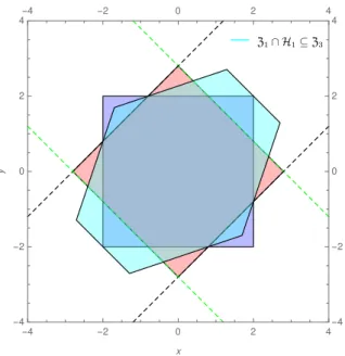
5.9 The zonotopic over-approximation of the intersection Z1X Z2 . . . 81

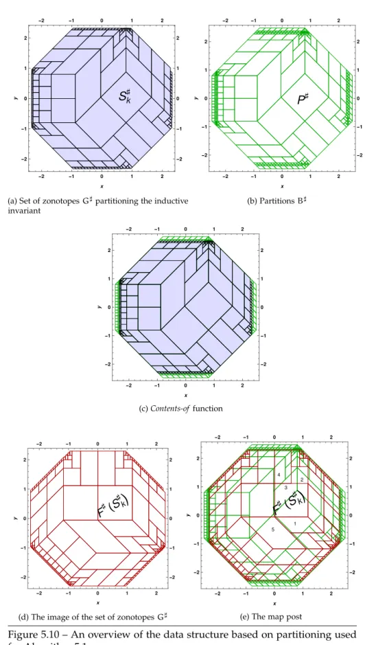
5.10 An overview of the data structure based on partitioning used for Algorithm 5.1 . . . 84

5.11 Sub-zonotopes obtained after splitting . . . 87

5.12 Computing the coverage measure in case of overlapping zonotopes 88 5.13 Split zonotopes for example 1 illustrating the issue with conven-tional coverage measure . . . 89

5.14 Inductive invariant for the program in Figure 2.6 with the target invariant being the box r´2, 2s abstracted using zonotopes . . . . 89

5.15 In red, the image of the zonotopes in Figure 5.14 by a loop iteration in the zonotope abstract domain and superposition of both showing that Figure 5.14 is inductive . . . 90

5.16 Partitioning and its effect on splitting by overlap . . . 91

5.17 Figures illustrating the ideas of fixing and freeing the signs of generators . . . 93

5.18 De Bruijn lines of a two-dimensional tiling. . . 95

5.19 Examples of tilings . . . 96

5.20 A hyperplane arrangment in R2_{with four lines. . . . 98}

5.21 Polar dual of the hyperplane arrangement in Figure 5.20, i.e., a zonotope. . . 99

5.22 A tiling of the zonotope in Figure 5.21 and the sign vectors of the corresponding tiles. . . 100

5.23 25 _{vertices of the 5-dimensional hypercube projected with the} generator matrix. . . 100

5.24 Arrangement of hyperplanes. . . 103

5.25 Ray shooting and sign enumeration. . . 103

5.26 The primitive zonotope and its tiling . . . 104

5.27 Illustrating, how fixing the sign of a zonotope defined by 3 genera-tors in 2-dimension implicitly enumerates all the tiles . . . 105

5.28 Illustrating, how fixing the sign of a zonotope defined by 4 genera-tors in 4-dimension implicitly enumerates all the tiles . . . 106

5.29 Illustrating one-by-one all sub-zonotopes obtained after fixing the sign of generators . . . 108

5.30 Illustrating one-by-one all parallelotopic tiles being enumerated . . 110

5.31 Illustrating one-by-one all sub-zonotopes obtained after fixing the sign of generators . . . 114

5.32 Illustrating one-by-one all parallelotopic tiles being enumerated . . 115

5.33 Illustrating one-by-one all parallelotopic tiles being enumerated . . 116

5.33 Illustrating one-by-one all parallelotopic tiles being enumerated . . 117

5.34 3-dimensional parallelotopic tiles delineating the zonotope in Fig-ure 5.31a. . . 117

6.1 Inductive invariant for Filter example . . . 122

6.1 Inductive invariant for Filter example . . . 123

6.2 Inductive invariant for Sine example . . . 124

6.2 Inductive invariant for Sine example . . . 125

6.3 Inductive invariant for Newton example . . . 126

6.3 Inductive invariant for Newton example . . . 127

6.4 Inductive invariant for Newton2 example . . . 128

6.4 Inductive invariant for Newton2 example . . . 129

6.5 Structure of a program for the analyzer . . . 131

7.1 Hénon attractor . . . 142

7.2 An outer-approximation of the positive invariant set of Hénon map (in blue are the abstract elements which are benign, in pink are the ones whose state cannot be decided by the algorithm, and in red is the image of the abstract elements by a loop iteration in the abstract domain used for computing the positive invariant set) . . 143

7.3 The set obtained using the CP Algorithm 7.1 upto a size criterion for an iterated function sequence F, F2_{. . . 144}

7.4 The set obtained using the CP Algorithm 7.1 upto a size criterion for an iterated function sequence F, F2_{, F}3_{. . . 145}

7.5 The set obtained using the CP Algorithm 7.1 upto a size criterion for an iterated function sequence F, F2_{, F}3_{, F}4_{. . . 146}

7.6 An outer-approximation of the positive invariant for the Van-der-Pol oscillator described by the map shown in Equation 7.31 . . . . 149 7.7 The image of abstract elements in Figure 7.6 by a loop iteration in

the abstract domain used for computing the positive invariant set 150 7.8 Superposition of the two figures 7.6 and 7.7 showing the abstract

elements which belong to the invariant set . . . 151 7.9 The set obtained using the CP Algorithm 7.1 upto a size criterion

for an iterated function sequence F, F2_{. . . 152}

7.10 The set obtained using the CP Algorithm 7.1 upto a size criterion for an iterated function sequence F, F2_{, F}3_{. . . 153}

7.11 The set obtained using the CP Algorithm 7.1 upto a size criterion for an iterated function sequence F, F2, F3, F4. . . 154 7.12 The set obtained using the CP Algorithm 7.1 upto a size criterion

for an iterated function sequence F, F2_{, F}3_{, F}4_{, F}5_{. . . 155}

7.13 Taylor model over-approximation for the function exppxq . . . 157 7.14 The set obtained after using our CP Algorithm on every new Taylor

model (6 order) evaluated at each time step over an interval r0, 5.20s.168 7.15 The set obtained after using our CP Algorithm on every new Taylor

model (6 order) evaluated at each time step over an interval r0, 6.70s.169 7.16 The set obtained after using our CP Algorithm on every new Taylor

model (7 order) evaluated at each time step over an interval r0, 6.80s.170

List of Tables

6.1 Experimental results with tightening applied only during first iteration. . . 120 6.2 Experimental results with tightening (tightening is applied after

each split). . . 130

List of Algorithms

4.1 A CP based AI algorithm for inferring inductive invariants [MBR16] 58 5.1 The zonotopic variant of the CP based AI algorithm 4.1 for inferring

inductive invariants . . . 71 5.2 Tiling Algorithm . . . 107 7.1 The zonotopic variant of the CP based AI algorithm 4.1 for inferring

inductive invariants while considering an iterated map sequence F, F2_{, ¨ ¨ ¨ , F}n _{. . . 140}

Pa r t I

I n t ro du c t i o n a n d S tat e o f

Chapter

1

Introduction

1.1 Motivation

Cyber-physical systems (CPS) are systems which combine the cyber world (computation/communication/data storage) with physical entities. A few examples of CPS are robots, cars, air-crafts, power plants, etc. With their ubiquitous presence in this society, verifying the correctness of programs and systems is becoming a major challenge.

In order to rely on them so as not to put our lives at stake, it is crucial to verify if they satisfy safety properties. For instance, an unmanned aerial vehicle (UAV) includes a mechanical body, remote ground control system, sensors (camera, inertial measurement unit, GPS, etc.), actuators, software and additional hardware like battery, electronic speed controller (ESC) and motors. All together it makes it a cyber-physical system. For such an UAV control system, it is important to verify if the UAV could potentially be involved in a collision within the next short period of time. This is where dynamical systems play a major role in approaches for studying whether a CPS satisfies crucial safety properties. They are mathematical models for describing temporal evolution of the state of a system.

Dynamical systems can contain discrete and continuous components. In discrete dynamical systems (or classical computer programs), the state evolves in discrete time steps, as described by difference equations. In continuous dynamical systems, the state of the system is a function of continuous time, characterized by differential equations. Determining the safety of a dynamical system requires to prove that the system is continuously safe.

A considerable part of this thesis is focused on developing method for the verification of safety properties of numerical programs. Additionally, we discuss the extension of this method to prove the safety properties for continuous time dynamical systems. In order to motivate the readers, we will present below a case study of verification of safety property of a computer program. However, prior to that we will recall the concepts from program verification that will constitute the background for all the chapters that follow.

1.1.1 Safety properties of programs

Ensuring whether or not a program satisfies a safety property is one of the widely studied fields in program verification. Various mathematical foundations aid the problem of program verification by providing proofs which help users to ascertain that a program is free from errors or behaves as

1.1. Motivation

intended. However, for any Turing complete programming language [Tur37] this problem is undecidable i.e., it is impossible to produce any sound and complete non-trivial assertion about the computational result of any program. That is Rice’s theorem [Ric53] which is a generalization of the well-known Halting problem [Tur37]. Partly the reason for this undecidability issue is loops. This is one of the reasons why analyzing loops is very crucial in program verification.

An informal definition of safety property is, “nothing bad happens” or “something bad never happens”, that is, a program never reaches an

unac-ceptable state. Safety properties on programs can be for instance, the fact that program variables stay within their expected bounds or some region is not reachable at some set of program locations. A safety property of interest express conditions that should be continuously maintained by the program. Hence, proving that a program satisfies a safety property of interest involves an invariance argument which is why loop invariants is a key ingredient in the verification of safety property on programs. An invariant is a property that holds on every iteration of the loop. Reasoning on invariants frees us from proving the safety of each loop iteration separately, which is costly for large loops and impossible for programs exhibiting unbounded loops and an infinite state space.

The classic method to prove that a set is indeed an invariant is to look for an inductive invariant which implies it, i.e., a state property that is stable by an iteration of the loop. An inductive invariant is an invariant (G) such that FpGq Ď G, as is used in, e.g., Floyd Hoare logic [Hoa69] [Flo67]. Further-more, Tarski’s theorem [Tar55] states that all inductive invariants are indeed invariants.

Inductive invariants play a special role in program verification because they can be checked by running a single loop iteration and checking its stability, even for unbounded loops. It is often necessary, given a target invariant property to prove, to first strengthen it into an inductive invariant.

We will motivate the importance of this thesis work further below with the illustration of a piece of code.

Example 1.1 We illustrate the concept of inductive invariants on a program in Figure 1.1 taken from the online additional material of [MBR16] (similar benchmarks are considered in [Mar14]) having two variables, x and y whose initial values lie in the box Idef“ r0.9, 1.1s2and the effect of a loop iteration on a set X of possible variable values px, yq P X given by the function F :PpR2_{q Ñ}

PpR2_{qdefined as the loop body of Figure 1.1.}

We choose an axis aligned bounding box such as G “ r´2.1, 2.1s ˆ r´2.1, 2.1s. Notice that the program state, considered as a point px, yq, is guaranteed to lie inside G every time that execution reaches the head of the loop. In other words, G includes notably all the states reachable at the loop head, i.e., Ť

nPN

Fn_{pIq Ď G. Then, the box G “ r´2.1, 2.1s ˆ r´2.1, 2.1s, shown}

in blue in Figure 1.2, is a valid invariant. However, notice that FpGq Ę G: indeed, the transformation induced by F on G maps the box G to a circle, that goes a bit outside the box G, as illustrated in Figure 1.2. Consider the four-petals-flower shape towards the center shown in Figure 1.2 : its interior is not reachable from the initial box I, and it contains the four small circles

1. Introduction

x =[0.9 ,1.1]; y =[0.9 ,1.1]; while ( True ) {

xnew =2x /(0.2 + x^2 + y^2 + 1.53 x^2y ^2); ynew =2y /(0.2 + x^2 + y^2 + 1.53 x^2y ^2); x= xnew ;

y= ynew ; }

Figure 1.1 – Example program.

-3 -2 -1 0 1 2 3 -3 -2 -1 0 1 2 3 x y

Figure 1.2 – Non-inductive invariants for the program in Figure 1.1.

in white which are the inverse image by F of the four parts of the circle that go beyond box G. The offending four small circles in the interior are not reachable program states. To prove this, using an axis aligned box, is not possible. Rather, we need to infer a stronger form of invariant, for e.g., inductive invariant that is included in G to prove that G is an invariant for executions beginning in I and precise enough to express that the small circles inside each petal of G are not reachable states.

One of the current techniques which provides a classical method to effec-tively compute inductive invariants in programs is Abstract interpretation (AI).

Abstract Interpretation. In general, AI is a theory of approximation of lattices. An abstract domain is chosen to represent effectively sets of pro-gram states. For environments over numeric variables, a wide set of abstract domains were proposed, such as boxes or intervals, polyhedras, octagons, zonotopes, ellipsoids, templates, etc. An abstract domain is adapted to a class of invariants we want to express (such as variable bounds) while abstracting away irrelevant information to improve efficiency. In other words, the abstrac-tion is made based on some property of interest. Then the funcabstrac-tion, modeling

1.1. Motivation

the effect of a loop iteration of the program is also abstracted using the same property. Now the inductive invariant is computed as limits of iterations of functions. However, for abstract domains which feature infinite increasing chain (for example, interval), these computations may fail to converge. In such a case, the classical solution would be to withdraw that particular domain and in its place redesign a new abstract domain which can represent the shape of the invariant. One may also use techniques like widening to enforce convergence, but this may come at the cost of precision.

In this thesis, we will focus on a particular abstract domain: zonotope.

Zonotope abstract domain. Zonotope is an implicitly relational abstract domain. It is based on affine forms. It is a cost-effective, versatile, and precise abstract domain that can represent restricted forms of polyhedra as Minkowski sums of line segments. It features more lightweight algorithms than general polyhedra, while being more expressive than other sub-polyhedra domains (e.g., octagons). They are particularly well suited to approximate non-linear functions. Zonotopes do not form a lattice and do not enjoy an exact intersec-tion. Thus, the major subject of this thesis is the introduction of new operators for this domain.

Another popular technique called constraint programming (CP), is used to find invariants by translating a program into constraints and solving them by using constraint solvers.

Constraint Programming. Constraint programming (CP) is a method for solving combinatorial problems, by expressing them as conjunctions of first-order logic formulas. It is a paradigm which formalizes invariant synthesis problem using constraints and solves them using efficient algorithms. These algorithms inherently know how to approximate a complex shape by a set of boxes, for instance, up to a precision criterion. Constraints in CP primarily operate on domains that are either discrete or continuous. Classical continuous constraint solving, over real-valued variables, works by refining the domain of the variables, i.e., a box representing candidate solutions: the box is tightened as much as possible by removing variable values that cannot participate in a solution. Whenever the box cannot be tightened anymore, it is split into two or more boxes, that are tightened and split themselves iteratively, until every box either contains only solutions, or no solution, or has a size below a user-defined threshold. When the algorithm terminates, it returns a set of definitive and candidate solutions as a collection of boxes.

Synthesizing invariants of programs has been an active research from early days of computer science, and recently many techniques which combine AI and CP have sprung up. In this thesis, we combine the zonotope based abstrac-tion with an existing CP algorithm [MBR16] for inferring inductive invariants. The idea of [MBR16], inspired from constraint programming approaches, is to synthesize an inductive invariant as a collection of abstract elements, that are iteratively split and refined. In set-based constraint programming, these elements are generally boxes. Previous work [MBR16] was limited to abstract domains that are closed by intersection and required non-standard opera-tions: split and size, such as octagons. In this thesis, we extend this work

1. Introduction -3 -2 -1 0 1 2 3 -3 -2 -1 0 1 2 3-3 -2 -1 0 1 2 3 -3 -2 -1 0 1 2 3 x y

(a) Inductive invariant obtained by our algorithm using boxes; -3 -2 -1 0 1 2 3 -3 -2 -1 0 1 2 3-3 -2 -1 0 1 2 3 -3 -2 -1 0 1 2 3 x y

(b) its image by a loop iteration;

-3 -2 -1 0 1 2 3 -3 -2 -1 0 1 2 3-3 -2 -1 0 1 2 3 -3 -2 -1 0 1 2 3 x y (c) octagons; -3 -2 -1 0 1 2 3 -3 -2 -1 0 1 2 3-3 -2 -1 0 1 2 3 -3 -2 -1 0 1 2 3 x y

(d) its image by a loop iteration;

Figure 1.3 – Inductive invariant found for the program in Figure 1.1

to zonotopes, which we show they provide an interesting trade-off between expressiveness and efficiency for such a use, by comparing their use with that of boxes, octagons, and polyhedra.

Example 1.2 Recall that no box is an inductive invariant for the program in Figure 1.1. The possible shapes1_{are as illustrated in Figures 1.3a, 1.3c, 1.3e}

and 1.3g. Instead of trying to guess the shape of the invariant, we will look for a set of abstract elements as shown in Figures 1.3a, 1.3c, 1.3e and 1.3g such that one iteration of the loop that is its image (shown in Figures 1.3b, 1.3d, 1.3f and 1.3h obtained by a computable abstract function modeling the effect

1.1. Motivation -3 -2 -1 0 1 2 3 -3 -2 -1 0 1 2 3-3 -2 -1 0 1 2 3 -3 -2 -1 0 1 2 3 x y

(e) polyhedra and

-3 -2 -1 0 1 2 3 -3 -2 -1 0 1 2 3-3 -2 -1 0 1 2 3 -3 -2 -1 0 1 2 3 x y

(f) its image by a loop iteration;

-3 -2 -1 0 1 2 3 -3 -2 -1 0 1 2 3-3 -2 -1 0 1 2 3 -3 -2 -1 0 1 2 3 x y (g) zonotopes and -3 -2 -1 0 1 2 3 -3 -2 -1 0 1 2 3-3 -2 -1 0 1 2 3 -3 -2 -1 0 1 2 3 x y

(h) its image by a loop iteration

1. Introduction

of a loop iteration on the abstract world) maps these set of abstract elements into a subset of itself as shown in Figure 2.4. Even though no single abstract element is an inductive invariant, a set of them can be inferred as an inductive invariant.

Figures 1.3a-1.3g show the inductive invariant within G as found by the CP algorithm in combination with box, octagon, polyhedron and zonotope abstract domains. Inference with intervals (resp. octagons, polyhedra, and zonotopes) takes 646.8 (resp. 8850.8, 126.8 and 35.6) seconds and produces an inductive invariant composed of 129781 (resp. 129767, 2368 and 488) parts. Less expressive domains such as boxes and octagons rely heavily on splitting, hence output a large set of elements and are slower in total, in spite of a smaller cost of manipulating a single abstract element. In particular, in polyhedra and zonotopes, the image by the loop body in the abstract domain, of a box on the left corner in Figure 1.3e-1.3g is within the collection of elements, thus proven invariant, whereas it won’t be the case in the box or octagon abstract domains, ultimately leading by splitting to the refinement of Figures 1.3a-1.3c.

Remark 1.3. An invariant associated with a safety property of interest can be relatively simple. For example, the value of a variable is bounded by so-and-so quantity. However, inductive invariants can have much more complex shapes as shown in Figures 1.3a-1.3g which makes them difficult to compute.

1.2 Our contribution

Our main goal during this thesis research was to extend an existing contin-uous constraint programming approach to domains which are not closed under intersection for synthesizing numerical invariants. More precisely, our contributions are:

• Zonotopes are not closed under intersection. So, we had to extend the existing framework, in addition to designing new operations on zonotopes, such as a novel splitting algorithm based on paving zonotopes by parallelotopes. We improved the complexity of the inclusion test on zonotopes by an exponential bound compared to the previous work. We also propose a new meet operation on zonotopes which is geometrical in nature. We implemented these operations in APRON library.

• We present a prototype that strengthens numerical invariants into induc-tive ones on a small language, extending the Taylor1+ zonotope abstract domain in the Apron library, and adapting the CP algorithm.

• We illustrate that the method is better than the previous one with an experimental proof on a small set of benchmarks.

• Finally, we show that our constraint programming framework can be used to find an over-approximation of positive invariants in continuous systems.

Some results described in Chapters 3 to 6 have been the subject of publi-cations in workshops [KGP16, KGP17, KGMP20]. We also co-wrote a paper discussing the new splitting operator for zonotopes and also the implementa-tion and experimentaimplementa-tion with Apron.

1.3. Thesis outline

1.3 Thesis outline

This thesis is organised as follows. Chapter 1 to 3 provide the requisite notions to understand this thesis research. Chapters 1 and 2 recall the concept of program invariants and gives an illustrative explanation as to why they must be inferred.

Chapter 2 recalls the formal framework of abstract interpretation and its application to infer inductive invariants of programs. It discusses the different abstract domains and the support libraries which implement their basic op-erations. This chapter also provides a brief survey on abstract interpretation based static analyzers. Chapter 3 gives the concepts of constraint program-ming. Chapter 4 discusses the recent continuous constraint programming approaches. It explains in detail an existing framework [MBR16] which com-bines AI and continuous CP inspired by an iterative refinement, splitting and tightening a collection of abstract elements. It will be extended throughout the thesis to be combined with the zonotope abstraction.

Chapter 5 defines the zonotope domain. It discusses how the constraint programming algorithm introduced in chapter 3 can be extended to domains that are not intersection-closed. It introduces new operators, such as a novel splitting algorithm based on tiling zonotopes by sub-zonotopes and parallelo-topes. It provides an extensive literature survey on tiling and the prerequisites to understand our tiling algorithm. It discusses the other zonotopic operators like meet, test for inclusion and intersection, and size that we needed to re-design in this context. Chapter 6 illustrates the experimental evaluation of our zonotopic abstraction based constraint programming method on programs with non-linear loops that present complex, possibly non-convex, invariants. Chapter 7 demonstrates how the CP framework can be extended to find invariants for continuous systems.

Chapter

2

Abstract Interpretation

In the previous chapter, we exemplified why inferring invariant sets is impor-tant. During this part of the thesis, we will be discussing the state-of-the-art methods for computing these sets. This chapter talks about a method which is a general theory for approximating the semantics of programs. The prominent static analysis approaches1 _{are based on this method, otherwise known as}

abstract interpretation (AI).

AI is an approach which computes properties of programs using math-ematical structures (lattices), transfer functions and fixed-points. Here, we discuss the key facts about abstract interpretation by introducing these mathe-matical structures and different fixed-point theorems. We also introduce the different existing abstractions (which are relevant to the present work) used by the AI framework for expressing numerical properties of programs.

2.1 Abstract interpretation

Recall that the main principle for proving that a property is an invariant for a loop of a program is to look for a stronger property that is an inductive invariant. The least (i.e. most precise) inductive invariant is the set of program states reachable from the initial states and can be expressed mathematically as a least fixpoint2. Computing this fixpoint using the real behavior of the program, or otherwise known as concrete semantics3 _{(more precise) is in}

general undecidable. Therefore, we have to rely on an interpretation which is based on less precise or abstract semantics but computable, and hence the name abstract interpretation [CC77]. It is a framework which expresses program semantics as fixpoints of functions over some ordered mathematical structures.

The relationship between the concrete semantics and abstract semantics is formally known as abstraction. For example, the abstraction of the concrete semantics could be the sign, or the range of the variables instead of their precise values. Different properties of a program can be represented by different abstract semantics. The different forms of abstraction over the

1_{These approaches analyze the program source code directly and without user intervention}

at some level of abstraction.

2_{A least fixpoint (a fixpoint is any a such that Fpaq “ a where F is a function F : A Ñ A}

and a P A) of a function which is a mapping from a mathematical structure to itself is a fixpoint smaller than one another fixpoint based on the structure’s order

3_{Semantics is the set of all possible executions in all possible environments. Informally, it is}

2.2. Notations and Definitions

semantics are known as abstract domains4. Denoted byD7_{such thatD}7

Ď PpRn_{q, an abstract domain is a subset of properties of interest with a computer}

representation, where PpRn

q or D is the concrete domain. The transfer function F7_{in the abstract domain i.e., F}7_:D7_ÑD7_{, over-approximates the}

effect of F :PpRn

q ÑPpRnq. Formally, this alternation between the concrete and abstract world can be defined by functions: an abstraction function from D to D7_{and a concretization function fromD}7_toD.

One of the widely used abstract domains is interval which abstracts set of points as a pair of bounds ra, bs where a ď b [CC76]. It is based on interval arithmetic [Moo69], quite simple and inexpensive, but non-relational. There are several other relational abstract domains like affine inequalities domain, or polyhedra domain [CH78] which integrates the ability of interval abstract domain in addition to the ability to infer relation among variables. This makes the polyhedra domain very expressive. There are other restrictions of polyhedra (weakly relational) like octagons [Min06], templates [SSM05] and zonotopes [GP06, GGP09] which rely on different algorithmic axioms. We will detail about the different abstract domains in the later part of this chapter. Henceforth, we introduce the basic concepts of abstract interpretation theory featuring the definitions of mathematical structures (partial order) and their relation to programs, characterizations about concept of fixpoints and a rich collection of fixpoint theorems. The readers can refer to [BCC`_{15, Min04,}

M`_{17, Gho11, Urb15] for more information.}

2.2 Notations and Definitions

We use standard notations from set theory: the empty set H, set union Y and intersection X, set inclusion Ď, set membership P, set difference z. Consider a set X, we denote asPpAq the set of all the sets included in X, otherwise known as powerset. Provided with two sets X and Y, the set of functions from X to Y is denoted by X Ñ Y. We use standard notation for introducing definitionsdef“or :“, logical operators: ^ for conjunction, _ for disjunction, =ñ for implication, ðñ for equivalence , |= for entailment and quantifiers: @for universal quantification, D for existential quantification. The set of real numbers, integers are denoted by R and Z respectively. Consider the sets S1, . . . , SkĎ Rn, then the Minkowski sum (denoted by ‘) of S1, . . . , Skis the

set S1‘ ¨ ¨ ¨ ‘ Sk“ ts1` ¨ ¨ ¨ ` sk| siP Siu. Consider two vectors x and y in Rn.

The inner product denoted by xpx1, x2, ¨ ¨ ¨ , xnq, py1, y2, ¨ ¨ ¨ , ynqyis given by

x1y1` x2y2` ¨ ¨ ¨ ` xnyn.

The `1norm of x is defined as

kxk₁def“

n

ÿ

i“1

|xi|.

4_{It is a computer-representable abstract version of the concrete domain to compute semantic}

2. Abstract Interpretation Consider a matrix M “ ˆ a c b d ˙

with column vectors. Its determinant is denoted by detpMq and is computed as

det ˆ a c b d ˙ “ ad ´ bc.

A Cartesian product of n intervals is a box given by B “ I1ˆ ¨ ¨ ¨ ˆ InConsider

a program with initial values or entry sets as I Ď Rn _{and a transfer function}

as F :D Ñ D where D: “ PpRn

qis the concrete domain.

Definition 2.1 (Concrete domain.) We are interested in inferring program invariants, i.e., properties of the state (mapping of each variable to its value) a program can be in at each program location. Thus, denoted byD, where D: “ PpRn

qa concrete domain corresponds to the values that can be taken by the variables throughout the program.

Definition 2.2 (Transfer function.) Provided with a precondition or an initial set of states, a transfer function F :PpRn

q ÑPpRnqmaps sets of environments to sets of environments after the execution of the line of code being analyzed. When the transfer function is applied to a set of environments X, we denote it by FpXq.

Definition 2.3 (Abstract domain.) Computing inPpRn

qcan be undecidable. Therefore we need a computer-representable abstract version of the concrete domain to compute semantic over-approximations. Thus denoted byD7_such

thatD7_ĎPpRn_{q, an abstract domain is a subset of properties of interest with}

a computer representation. The computable abstract function F7_{: D}7 _ÑD7

over-approximates the effect of F :D Ñ D.

Definition 2.4 (Partially ordered set or poset.) A partial order Ď on a set X is a relation which satisfies the following axioms:

• Reflexive: @x P X : x Ď x

• Anti-symmetric: @x, y P X : px Ď yq ^ py Ď xq Ñ x “ y • Transitive: @x, y, z P X : px Ď yq ^ py Ď zq Ñ x Ď z

The set X armed with such a partial order relation5 _{Ďis called a partially}

ordered set or poset and can be denoted as the pair pX, Ďq.

Remark 2.5. Partial orders are very crucial in theoretical computer science, but they also provide a mathematical foundation in programs. Consider a program prog which satisfies a specification spec, i.e., a property of the program. One of these properties could be for instance, values of any variable of prog during execution is always between a particular bound. That means, whether or not the program prog satisfies the specification spec is equivalent to a set inclusion problem, i.e., if prog Ď spec.

Definition 2.6 (Complete partial order.) A poset pX, Ďq is called complete partial order or CPO if every totally ordered subset (M Ď X) in the poset X has

5_{A binary relation can also be pre-order, if a relation is reflexive, transitive, but not necessarily}

2.2. Notations and Definitions

a least upper bound, where totally ordered means px Ď yq _ py Ď xq @x, y P M. When a poset pX, Ďq is a CPO then it is denoted as pX, Ď, \q

Remark 2.7. A totally ordered subset of a poset is otherwise known as a chain.

Definition 2.8 (Lattice.) A lattice is a poset (L,Ď,\,[) where every collection of elements has a least upper bound, denoted by \ and a greatest lower bound, denoted by [. For example, consider any two elements a, b PL there is a least upper bound or join, i.e., a \ b, and a greatest lower bound, i.e., a [ b. We can claim that the latticeL is complete if every subset M of L has a least upper bound \M and a greatest lower bound [M and L has a least element K6_.

Definition 2.9 (Monotonicity & Continuity.) Consider two posets pD1, Ď1q

and pD2, Ď2q. A function F : pD1, Ď1q Ñ pD2, Ď2qis called a monotonic function

if xĎ1y =ñ FpxqĎ2Fpyq@x, y P D1.

Consider two complete partial orders pD1, Ď1, \1q and pD2, Ď2, \2q. A

function F : pD1, Ď1, \1q Ñ pD2, Ď2, \2qis said to be a continuous function if

for every chain C Ď D1, FpCq is also a chain, i.e., FpCq Ď D2, and Fp\1Cq “

\2FpCq.

Definition 2.10 (Fixpoints.) Consider a partially ordered set pY, Ďq and a function F which is a mapping from the poset to itself, i.e., F : Y Ñ Y. A fixpoint of a transfer function F is any element X satisfying FpXq “ X | X P Y. A pre-fixpoint X is such that FpXq Ě X and a post-fixpoint X such that FpXq Ď X. We denote the least fixpoint of F as lfpXFwhich is defined as

lfpXF “ [tF’s post-fixpoints larger than Xu (2.1)

We will denote the greatest fixpoint of F by gfpXFwhich is defined as

gfpXF “ \tF’s pre-fixpoints smaller than Xu (2.2)

The existence of a least fixpoint and the fact that it is the meet of all the post-fixpoints, both follow from Tarski’s theorem [Tar55] defined below. Definition 2.11 (Tarski’s theorem.) If F :L Ñ L is a monotonic function on a complete latticeL, then the set of fixpoints of F is a non-empty complete lattice and a least fixpoint exists.

Remark 2.12. Among the set of fixpoints, the least fixpoint is the smallest and unique, if exists. It can refer to critical parts of the semantics of a program. Below, we will illustrate the post-fixpoint of a computer program.

Example 2.13 Consider a simple program shown in Figure 2.1(a) taken from [MBR16, Fer04] having two variables, s0 and s1, and its loop that implements

a second order digital filter. The variables s0 and s1are initially set to values

in r´0.1, 0.1s. The numbers 1.5, ´0.7 are the coefficients of the filter. At each loop iteration, the variable s0denotes the value of the current filter output, the

variable s1denotes the last value of the filter output and the interval r´0.1, 0.1s

denotes the value of the current filter input.

6_{K(also called bottom) and J (also called top) are the least and greatest elements of a poset, if}

2. Abstract Interpretation s0=[ -0.1 ,0.1]; s1=[ -0.1 ,0.1]; while ( True ) { r = 1.5* s0 - 0.7* s1 + [ -0.1 ,0.1]; s1 = s0; s0 = r; }

Figure 2.1 –(a) Example program; (b) The reachable states (s0, s1) form an ellipsoid

The initial values of variables ps0, s1q are in the box I

def

“ r´0.1, 0.1s ˆ r´0.1, 0.1s and the effect of a loop iteration on a set X of possible variable values ps0, s1q P Xgiven by the function F :PpR2q ÑPpR2qdefined as FpXq

def

“ tp1.5 ˆ s0´0.7 ˆ s1` r´0.1, 0.1s, s0q|ps0, s1q P Xu. The evaluation of the interval

r´0.1, 0.1s can be inferred as picking a different value between -0.1 and 0.1 at each loop iteration. This indeterminacy in the evaluation of the interval makes the program non-deterministic.

For the above program semantics, a set G Ď Rn_{(here n “ 2) can be claimed}

as inductive invariant if I Ď G ^ FpGq Ď G with the least fixpoint of F or lfpIF

being the smallest one. In that case any set G satisfying that G Ě lfpIFis an

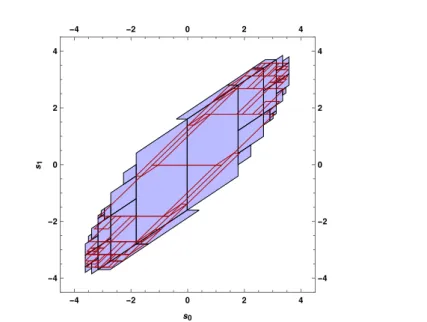
invariant which means that all inductive invariants are invariants but not all invariants are always inductive. Notably, the set of program states reachable from the initial states is the least (i.e. most precise) inductive invariant as illustrated in Figure 2.1(b). Generally, this set is difficult to compute, so we settle for an over-approximation, as any such over-approximation is also an invariant. In other words, any post-fixpoint of F is a sound over-approximation of the least fixpoint of F because lfp_IF is characterized as the meet of all post-fixpoints. Thus, any post-fixpoint is a constructive expression for an inductive invariant. A post-fixpoint for the program in Figure 2.1(a) is shown in Figures 2.2-2.4.

Remark 2.14. Note that in this thesis work, given a target invariant property to prove, we first strengthen it into an inductive invariant.

Abstract interpretation provides tools to infer inductive invariants. For instance, as the limit of an iteration sequence. We discuss this below in detail. Remark 2.15. Although Tarski’s theorem ensures the existence of least fixpoint, it does not provide any ground rule on how to compute them effectively. In other words, it does not say how a post-fixpoint can be computed in abstract, where the least fixpoint being the meet of all the post-fixpoints. Thus, one of the variants of fixpoint approximation theorem is a classical method based on the work of Kleene et al. [KdBdGZ52] was provided by Cousot and Cousot [CC77] to infer inductive invariants, which states that least fixpoints can be

2.2. Notations and Definitions -4 -2 0 2 4 -4 -2 0 2 4 -4 -2 0 2 4 -4 -2 0 2 4 s0 s1

Figure 2.2 – Inductive invariant for the program in Figure 2.1

-4 -2 0 2 4 -4 -2 0 2 4 -4 -2 0 2 4 -4 -2 0 2 4 s0 s1

Figure 2.3 – The image of abstract elements in Figure 2.2 by a loop iteration in the abstract domain used for computing the inductive invariant

2. Abstract Interpretation -4 -2 0 2 4 -4 -2 0 2 4 -4 -2 0 2 4 -4 -2 0 2 4 s0 s1

Figure 2.4 – Superposition of the two figures 2.2 and 2.3 showing that 2.3 is included in 2.2, i.e., 2.2 is inductive

computed as limits of iterations, or otherwise known as Kleene’s theorem [Def. 2.16].

Definition 2.16 (Kleene’s Theorem.) If F :L Ñ L is a continuous function in a complete partial orderL, then least fixpoint exists and it can be expressed as:

lfp_KF “ \ FipKq | i PN( (2.3) whereN is the set of natural integers.

Remark 2.17. Unlike Tarski’s fixpoint theorem, Kleene’s fixpoint theorem [KdBdGZ52, CC77, CC79] requires only a complete partial order and more intriguing is the fact that it characterizes the least fixpoint as a limit of value iteration. This iteration is guaranteed to converge provided the complete partial order has no infinite strictly increasing chain. Consider computing these iterates pK, FpKq, FpFpKqq, ¨ ¨ ¨ , Fn_{pKq, ¨ ¨ ¨ q of K which may converge but}

to a useless one, i.e., J. To address this convergence issue, Cousot and Cousot [CC77] introduced a widening operator ∇.

Kleene iteration. An abstract domain is chosen to represent effectively specific sets of program states, such as boxes or convex polyhedra for envi-ronments over numeric variables. It is adapted to a class of invariants we want to express (such as variable bounds) while abstracting away irrelevant information to improve efficiency. Then, a computable abstract function F7

modeling the effect of a loop iteration on the abstract world is defined (e.g., a function from boxes to boxes). The inductive invariant is computed as the limit of a Kleene iteration sequence, iterating F7 _{from an abstract}

represen-tation I of the set of states before entering the loop of a program: X0 _{“ I,}

@k.Xk`1 _{“ X}k

Y7F7_pXk_{q. In general, this sequence does not terminate. A}

num-2.2. Notations and Definitions -50 0 50 100 -50 0 50 -50 0 50 100 -50 0 50 s0 s1

Figure 2.5 – Kleene iterations in the interval domain

ber of iterations, we find an abstract inductive invariant Xk`1_{Ď X}k_{. However,}

the widening operator can lead to loss of precision.

Below, we will consider again the program in Figure 2.1(a) and illustrate the Kleene iterations for inferring inductive invariant.

Example 2.18 Consider a box G “ r´4, 4s ˆ r´4, 4s. G is a valid invariant for the program in Figure 2.1(a) because G includes notably all the program states reachable at the loop head. On the domain of boxes, the kleene iteration will continue with larger oxes, as shown in Figure 2.5, until it is widened to r´8, `8s2_{, which does not imply our invariant G: the method fails as no box}

is an inductive invariant (the transformation induced by F on G makes its corners overflow G).

Remark 2.19. As of now, we have discussed Kleene iteration based fixpoint computation. Below we will review one of its type, which is rather based on policy iteration7 _{and not value iteration}8_.

Policy or strategy iterations. The inductive invariants (of course not the strongest one) in programs can be expressed as a post-fixpoint. In the static analysis community, Kleene iterations with widening is a well-known approach for computing these fixpoint overapproximations [CC77]. Another approach which solves similar problems, is policy iteration [AGG10]. For instance, the policy iterations with ellipsoid abstract domain has been more

7_{In general, policy iteration algorithms start with a random policy, then finds the value}

function of that policy, and then finds a new or improved policy based on the previous value function.

8_{In value iteration, one starts with a random value function and then improves the value}

function in an iterative way, until reaching the optimal value function. In value iteration, once the value function reaches its optimal value, the policy out of it is optimal.

2. Abstract Interpretation

effective in inferring quadratic invariants compared to Kleene iterations with ellipsoids [RG14].

The idea is to use appropriate mathematical solvers to solve the fixpoint equation for a given abstract domain using policy iterations instead of optimal value iteration (like Kleene). For instance, if the abstract domain and the fixpoint equation use quadratic equations then semi-definite programming is considered [AGG10]. Similarly, if linear equations are used then one can benefit from linear programming [GGTZ07]. Thus, thanks to these solvers that one can compute the solution without using the convergence techniques. The policy iterations are otherwise known as strategy iterations [GS07a, GS07b, GSA`_{12]. Both the iterations aim at fixpoint computation by a}

sym-bolic reasoning based on mathematical solvers like semi-definite programming. However, there is a minor difference in between the two iterations with respect to the policies on which they iterate. For instance, in strategy iterations, one iterates on max-policies, starting from bottom and increasing the bounds until the fixpoint is reached, whereas policy iterations iterate on min-policies, starting from an over-approximation and decreasing the bounds until the fixpoint is attained. Thus, these approaches can be seen as an alternative to Kleene iterations with widening.

There is a recent work [KMW16] which is based on max-policies and formulates the policy iteration as traditional Kleene iteration, with a widening operator.

Both the iterations require templates (appropriate shapes) to be given prior to the analysis. Thus, before using any abstract domain with policy iterations, it must be expressed in terms of template domains. This no doubt makes the method less automatic. Also, the quality of the fixpoint reached by either of the iterations depend on the initial policy used [RJGF12, RG14].

Definition 2.20 (Concretization & Abstraction function.) Consider two posets: pD, ďq representing the concrete world and pD7_{, Ďq, the abstract world.}

A concretization function γ :D7_{ÑD is a monotonic function which converts}

each abstract element inD7_{to a concrete one.}

Consider a reverse function, called an abstraction function denoted by α which converts from a concrete world back to an abstract one, i.e., α :D Ñ D7_.

Definition 2.21 (Widening.) Widening, on an abstract domain pD7_{, Ďq is an}

operator ∇ :D7_ˆD7_ÑD7_{such that:}

• @x, y PD7_{: x, y Ď px∇yq, and}

• for any sequence xi P D7 where i P N, the increasing sequence yi

calculated as

y0:“ x0, yi`1:“ yi∇xi`1

stabilizes after a finite number of iterations, i.e., Dk ě 0 : yk`1“ yk.

Definition 2.22 (Galois connection.) Consider two posets pX, ďq (concrete) and pY, Ďq (abstract), an abstraction function α : X Ñ Y, a concretization function γ : Y Ñ X and @x P X, y P Y : αpxq Ď y ðñ x ď γpyq then the pair xα, γy is a Galois connection denoted by:

pX_{, ďq ´´´Ñ}д´´

α γ

2.3. Numerical abstract domains

Remark 2.23. An essential property established by Galois connection is the strong connection between the concrete and the abstract world. However, not all abstract domains enjoy a Galois connection because they may not have an explicit α which is why the minimum requirement to interact between the two worlds is to at least have a concretization function γ. This is what is called the soundness property through concretization function.

Definition 2.24 (Soundness property.) Consider a concretization function γ : pD7_{, Ďq Ñ pD, ďq, a concrete transfer function F: D Ñ D, and an abstract}

transfer function F7_:D7_ÑD7_{. The function F}7_{is called a sound abstraction}

of F if @x PD7_{: Fpγpxqq ď γpF}7_pxqq.

2.3 Numerical abstract domains

In general, computing in concrete domainD: “ PpRn

qcan be undecidable because the set of environments may need infinite memory to be represented exactly, and computation of the set of locations infinite time. Therefore, we reason in an approximation (abstract domain) where we forget some of the properties of the concrete semantic domain (or in other words subset of properties of interest) in order to get the domain computable and machine-representable. LetD7_{be the abstract domain such that}D7_ĎPpRn_{q. To define}

an abstract domainD7_{one needs to characterize the following:}

• a partial order Ď7_onD7_,

• a concretization function γ :D7_ÑD,

• a Galois connection, which is optional because there may not exist an abstraction function α : D Ñ D7 to form a Galois connection pD, ď

q ´´´Ñд´_α´

γ

pD7_{, Ď}7_{q. However, what we require at least is the soundness}

property, i.e., properties of program proved to hold in abstract domain also holds in the concrete one, when we do not have an abstraction function ,

• a join operator Y7_{(an abstraction of set union Y) and a meet operator}

X7(an abstraction of set intersection X) over the abstract elements,

• a smallest element K7_{and a largest element J}7_,

• a widening operator ∇7_.

Finally, we must note that the abstract domain needs only have a poset structure, but not necessarily a CPO nor a lattice.

Many numerical abstract domains are developed because different domains can be used to obtain different properties of programs. The major ones are intervals [CC76] and polyhedra [CH78]. There are many new abstract domains been developed over these years, capturing other properties, such as octagons [Min06], template [SSM05], zonotopes [GP06, GGP09] and ellipsoids [Fer04].

2. Abstract Interpretation

2.3.1 Non-Relational Abstract Domain

The abstract domains of this family are the least expressive. They abstract the set of possible values of each variable independently of the other variables, and hence the name. The well-known in this area is the interval abstract domain. It is based on interval arithmetic, introduced by Moore [Moo69] for numeric analysis, and later adapted to static analysis by Cousot and Cousot [CC76] with the inception of abstract interpretation.

The interval abstract domain, as its name implies, represents each variable as an interval of its possible values, for e.g., ra, bs with a ď b. It represents several variables by using a Cartesian product defined as śni“1rai, bis | @i :

ai, biP R Y t´8, 8u(. Even though it is a non-relational domain, but yet it is

simple and inexpensive to implement, and also it can infer useful properties for program verification. However, being an abstract domain with strictly infinite increasing chains, it requires widening to enforce convergence. Cousot et al. in [CC76] showed that an interval analysis can over-approximate least fixpoint with widening.

The basic operations available in the interval abstract domain are:

• concretization: γpra, bsqdef“ _{x P R | a ď x ď b}(

• ordering: ra, bsĎ7_{rc, ds ðñ pa ě cq ^ pb ď dq (semantically equivalent}

to set inclusion, i.e., ra, bs Ď rc, ds)

• join: ra, bsY7_{rc, ds}def_{“ rminpa, cq, maxpb, dqs}

• meet: ra, bsX7_{rc, ds}def_“

#

rmaxpa, cq, minpb, dqs, if maxpa, cq ď minpb, dq K7, otherwise

• addition: ra, bs`7<sub>rc, ds</sub>def<sub>“ ra ` c, b ` ds</sub>

• subtraction: ra, bs´7def

“ ra ´ d, b ´ cs

• multiplication: ra, bsˆ7def_{“ rminpac, ad, bc, bdq, maxpac, ad, bc, bdqs}

• divison: ra, bs{7_{rc, ds}def_“

$ ’ & ’ %

rminpa{c, a{dq, maxpb{c, b{dqs, if 1 ď c rminpb{c, b{dq, maxpa{c, a{dqs, if d ď ´1 pra, bs{7_{prc, dsX}7_{r1, `8sqqY}7_{pra, bs{}7_{prc, ds X}7_{r´8, ´1sqq, otherwise}

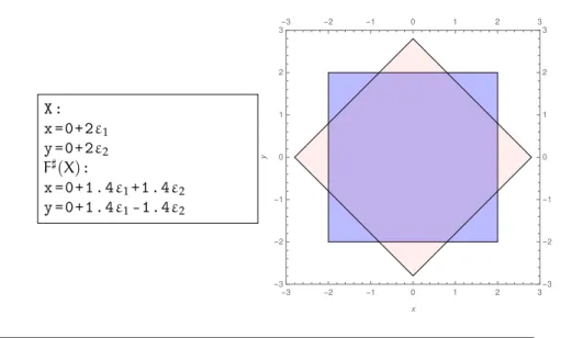
Example 2.25 Consider a program shown in Figure 2.6 having two variables, x and y, and its loop body performs a rotation of the point px, yq about the origin, with a minor scaling penetrating inward. The initial values of variables px, yq are in the box Idef“ r´1, 1s ˆ r´1, 1s and the effect of a loop iteration on a set X of possible variable values px, yq P X given by the function F :PpR2q ÑPpR2qdefined as FpXqdef“ tp0.7 ˆ px ´ yq, 0.7 ˆ px ` yqq|px, yq P Xu. Provided with an interval r´2, 2s, we can define an axis aligned bounding box such as X “ r´2, 2s ˆ r´2, 2s shown in Figure 2.7 in blue. The image of this box by a loop iteration in the interval domain is F7_{pr´2, 2s, r´2, 2sq}def_“

2.3. Numerical abstract domains x=[ -1 ,1]; y=[ -1 ,1]; while ( True ) { xnew =0.7*( x + y); ynew =0.7*( x - y); x= xnew ; y= ynew ; }

Figure 2.6 – Example program

X: x P [ -2 ,2]; y P [ -2 ,2]; F7_pXq: x P [ -2.8 ,2.8]; y P [ -2.8 ,2.8]; -3 -2 -1 0 1 2 3 -3 -2 -1 0 1 2 3-3 -2 -1 0 1 2 3 -3 -2 -1 0 1 2 3 x y

Figure 2.7 –(a) The interval abstract values for the target invariant of the program in Figure 2.7 and its image after one iteration of the body loop; (b) In blue: the target invariant (X), in pink: F7_pXq.

pr0.7p´2´2q, 0.7p2`2qs, r0.7p´2´2q, 0.7p2`2qsqq, which is the box in Figure 2.7 in pink.

2.3.2 Relational Abstract Domains

Presumably, very often, for simple programs, the bound information provided by interval abstract domain is sufficient. However, it does not guarantee the tightest possible bounds. This led to the development of relational domains (more expressive) which incorporate the properties inferred by non-relational domains in conjunction with affine relationships among variables of a program. One of the most widespread relational domains is affine inequalities domain or polyhedra.

Polyhedras. The polyhedra abstract domain was introduced by Cousot and Halbwachs [CH78]. As the name suggests, this domain abstracts a set of

2. Abstract Interpretation

points in the form of a convex polyhedron9. Recall that the existence of a best abstraction is useful but not necessary. One of the examples is the polyhedra domain which can abstract set of points as an unbounded convex polyhderon.

No Galois connection. There is no Galois connection for a polyhedra because it lacks an abstraction function or has no best abstraction as a poly-hedron. The reason for no abstraction function is owing to shapes, such as circles, which do not have a smallest enclosing polyhedron. In other words, we can have an infinity number of tangents to the circle leading to the existence of a polyhedron with infinite number of constraints approximating the circle. Few important results of polyhedra theory are the Farkas-Lemma and the Weyl-Minkowski Theorem [Wey34, Sch98], which state that polyhedras have dual representations: one using constraints, and one using generators. For a subsetP (polyhedron) of Rn_{, the following definitions are equivalent:}

Definition 2.26 (H-Representation or exterior representation) A polyhe-dron is defined as the intersection of finitely many halfspaces, i.e., there exists a matrix A and a vector b with

P “ x P Rn

| Ax ď b( (2.4)

where the halfspaces are represented by the inequalities Ax ď b and n being the number of abstracted numerical variables. In other words, the polyhedronP is the solution set x P Rn_{to a finite system of linear inequalities.}

Definition 2.27 (V-Representation or interior representation) Given a finite a set of extremal points or vertices (si, 1 ď i ď k orS) and a finite set of

extreme directions or rays (tj, 1 ď j ď m orT) a polyhedron can be defined as

P “ convpSq ` conepTq (2.5) where convpYq denotes the convex hull of a set Y Ď Rn _{defined by}

convpYq “ ! _ÿ yPY1 αyy : Y1Ď Y, |Y1| ă 8, ÿ yPY1 αy“1, αyě0@y P Y1 ) (2.6)

In other words, any point x PP can be represented as, x “ k ÿ i“1 λisi` m ÿ j“1 βjtj (2.7) where λiě0, βjě0, řk i“1λi“1.

A bounded polyhedron can be constructed simply by taking convex hull of finite set of vertices. The definition by Equation (2.5) is more general, i.e., by adding rays furthermore, one can obtain an unbounded polyhedron. Switching between the two representations is a well-known result in the polyhedral theory. Changing from H-representation to V-representation is a vertex enumeration problem and the contrariwise is a facet enumeration problem. The best representation varies from one operator to the other. For

9_{Polygon is a two-dimensional polytope. Polyhedra or polyhedron is a three-dimensional}