Linear Logic and Sub-polynomial Classes of Complexity

HAL Id: tel-00957653

https://tel.archives-ouvertes.fr/tel-00957653v2

Submitted on 9 Nov 2014

HAL is a multi-disciplinary open access

archive for the deposit and dissemination of

sci-entific research documents, whether they are

pub-lished or not. The documents may come from

teaching and research institutions in France or

abroad, or from public or private research centers.

L’archive ouverte pluridisciplinaire HAL, est

destinée au dépôt et à la diffusion de documents

scientifiques de niveau recherche, publiés ou non,

émanant des établissements d’enseignement et de

recherche français ou étrangers, des laboratoires

publics ou privés.

Distributed under a Creative Commons Attribution - NonCommercial - ShareAlike| 4.0

International License

Clément Aubert

To cite this version:

Clément Aubert. Linear Logic and Sub-polynomial Classes of Complexity. Computational Complexity

[cs.CC]. Université Paris-Nord - Paris XIII, 2013. English. �tel-00957653v2�

Sorbonne Paris Cité

Laboratoire d’Informatique de Paris Nord

Logique linéaire et classes de complexité

sous-polynomiales

k

Linear Logic and Sub-polynomial Classes of

Complexity

Thèse pour l’obtention du diplôme de

Docteur de l’Université de Paris :3,

Sorbonne Paris-Cité,

en informatique

présentée par Clément Aubert

<

[email protected]

>

F

=

f

Mémoire soutenu le mardi 26 novembre 20:3, devant la commission d’examen composée de :

M.

Patrick Baillot

C.N.R.S., E.N.S. Lyon

Rapporteur

M.

Arnaud Durand

Université Denis Diderot - Paris 7

Président

M.

Ugo Dal Lago

I.N.R.I.A., Università degli Studi di Bologna Rapporteur

Mme. Claudia Faggian

C.N.R.S., Université Paris Diderot - Paris 7

M.

Stefano Guerrini

Institut Galilée - Université Paris :3

Directeur

M.

Jean-Yves Marion

Lo.R.I.A., Université de Lorraine

M.

Paul-André Melliès C.N.R.S., Université Paris Diderot - Paris 7

M.

Virgile Mogbil

Institut Galilée - Université Paris :3

Co-encadrant

F

=

f

Errata

S

omeminor editions have been made since the defence of this thesis (improvements in the bibliog-raphy, fixing a few margins and some typos): they won’t be listed here, as those errors were not altering the meaning of this work.:

However, while writing an abstract forTERMGRAPH 20:4, I realized that the simulation of Proof Circuits by an Alternating Turing Machine, in theSection 2.4ofChapter 2was not correct.

More precisely, bPCCi _{is not an object to be considered (as it is trivially equal to PCC}i_{) and}

Theorem 2.4.3, p.5:, that states that “For all i > 0, bPCCi

⊆ STA(log,∗,logi_{)”, is false. The ATM}

constructed do normalize the proof circuit given in input, but not within the given bounds. This flaw comes from a mismatch between the logical depth of a proof net (Definition 2.:.:0) and the height of a piece (Definition 2.2.6), which is close to the notion of depth of a Boolean circuit (Definition 2.:.2).

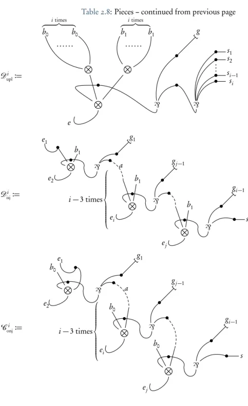
First, remark that the class bPCCi_{(Definition 2.2.8) is ill-defined: recall that (Lemma 2.3.:) in the}

case of Dk

isjand Conjk pieces, one entry is at the same logical depth than the output, and all the other

entries are at depth 3 plus the depth of the output.

In the process of decomposing a single n-ary operation in n − 1 binary operations, the “depth-efficient way” is not the “logical depth-efficient way”. Let us consider a tree with n leafs (f) and two ways to

organize it:

f f f f f f f f f f

f f

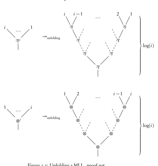
Let us take the distance to be the number of edges between a leaf and the root of the tree. Then, on the left tree, every leaf is at the same distance log(n), and on the right tree, the greatest distance is n. Everything differs if one consider that every binary branching is a D2

isjor Conj2 piece and consider the

logical depth rather than the distance. In that case, on the left-hand tree, the ith leaf (starting from the left) is at logical depth 3 times the number of 1 in the binary encoding of i.2_{On the right-hand tree,} every leaf is at logical depth 3, except for the red leaf (the left-most one), which is at logical depth 0. So the logical depth is in fact independent of the fan-in of the pieces, and it has the same “logical cost” in terms of depth to compute Di

isjor Conji for any i ¾ 2. A proof circuit of PCCiis a proof circuit of

bPCCi_{: every piece of P}

u can be obtained from pieces of Pb without increasing the logical depth. So

we have that for all i ∈ N, PCCi=bPCCi.

Secondly, the proof ofTheorem 2.4.3was an attempt to adapt the function value(n, g, p) [:35, p. 65]

that prove that an ATM can normalize a Boolean circuit with suitable bounds. The algorithm is correct,

:_{Except maybe for a silly mistake inProposition 4.3.:, spotted by Marc Bagnol.}

2_{Sic. This sequence is known asA000:20and starts with 0,1,1,2,1,2,2,3,1,2,2,3,2,3,3,4,....}

but not the bounds: it is stated that “Each call to f uses a constant number of alternations, andO(d (Pn))

calls are made. As Pnis of depth logi(n),O(logi(n))calls are made.”, and this argument is wrong.

Consider that Pn∈ PCCi(this is harmful taking the first remark into account), when the ATM calls f

to evaluate the output of a Dk

isjor Conjk piece, it makes k − 1 calls to f at a lesser depth, and one call at

the same depth. The only bound on the fan-in of the pieces, k, is the size of the proof circuit, that is to say a polynomial in the size of the input: this is a disaster.

tl;dr: bPCCishould not be considered as a pertinent object of study and the correspondence between the proof circuits and the Alternating Turing Machines is partially wrong. This does not affect anyhow the rest of this work and this part has never been published nor submitted.

Disclaimer:It is not possible for me to write these acknowledgements in a language other than French. Remerciements. Il est d’usage de commencer par remercier son directeur de thèse, et je me plie à cet usage avec une certaine émotion : Stephano Guerrini m’a accordé une grande confiance en acceptant de m’encadrer dans cette thèse en Informatique alors que mon cursus ne me pré-disposait pas tellement à cette aventure. Par ses conseils, ses intuitions et nos discussions, il a su m’ouvrir des pistes, en fermer d’autres, conseiller et pointer de fructueuses lectures.

Virgile Mogbil a co-encadré cette thèse avec une attention et un soin qui m’ont touchés. Il a su m’accompagner dans tous les aspects de celles-ci, m’initier à la beauté de la recherche sans me cacher ses défauts, me guider dans le parcours académique et universitaire bien au-delà de ma thèse. Il su faire tout cela dans des conditions délicates, ce qui rend son dévouement encore plus précieux.

Patrick Baillot fût le rapporteur de cette thèse et comme son troisième directeur : il a su durant ces trois années me conseiller, me questionner, chercher à comprendre ce que je ne comprenais pas moi-même. C’est un honneur pour moi qu’il ait accepté de rapporter ce travail avant autant de justesse et de clairvoyance.

Je suis également ravi qu’Ugo Dal Lago ait accepté de rapporter ce travail, et m’excuse pour l’avalanche de coquilles qui ont dû lui abîmer l’œil. Sa place centrale dans notre communauté donne une saveur toute particulière à ses remarques, conseils et critiques.

Je suis honoré qu’Arnaud Durand — qui fût mon enseignant lorsque je me suis reconverti aux Mathématiques — ait accepté d’être le président de ce jury. La présence de Claudia Faggian, Jean-Yves Marionet Paul-André Melliès place cette thèse à l’interscetion de communautés auxquelles je suis ravi d’appartenir. Je les remercie chaleureusement pour leur présence, leurs conseils, leurs encouragements.

Une large partie de ce travail n’aurait pas pu voir le jour sans la patience et la générosité de Thomas Seiller, avec qui j’ai toujours eu plaisir à rechercher un accès dans la compréhension des travaux de Jean-Yves Girard.

§

Mon cursus m’a permis de rencontrer de nombreux enseignants qui ont tous, d’une façon ou d’une autre, rendu ce cheminement possible. J’ai une pensée particulière pour Louis Allix, qui m’a fait découvrir la logique et pour Jean-Baptiste Joinet, qui a accompagné, encouragé et rendu possible ce cursus. De nombreux autres enseignants, tous niveaux et matières confondus, m’ont fait aimer le savoir, la réflexion et le métier d’enseignant, qu’ils m’excusent de ne pouvoir tous les nommer ici, ils n’en restent pas moins présents dans mon esprit.

§

J’ai été accueilli au Laboratoire d’Informatique de Paris Nord par Paulin Jacobé de Naurois (qui encadrait mon stage), Pierre Boudes et Damiano Mazza (qui ont partagé leur bureau avec moi), et je ne pouvais rêver de meilleur accueil. L’équipe Logique, Calcul et Raisonnement offre un cadre de travail amical et chaleureux dans lequel je me suis senti accompagné, écouté et bienvenu.

Devenir enseignant dans une matière que je connaissais mal (pour ne pas dire pas) aurait été une tâche insurmontable pour moi si elle n’avait eu lieu à l’IUT de Villetaneuse, où j’ai trouvé une équipe dy-namique et respectueuse de mes capacités. Laure Petrucci, Camille Coti, Jean-Michel Barrachina, Fayssal Benkhaldoun et Emmanuel Viennet m’ont tous énormément appris dans leur accompagne-ment patient et attentif.

Ce fût toujours un plaisir que de discuter avec mes collègues du L.I.P.N., ainsi qu’avec le personnel administratif de Paris :3. Brigitte Guéveneux, tout particulièrement, sait marquer de par sa bonne humeur et son accueil chaleureux tout personne qui pénètre dans ces locaux, qu’elle en soit remerciée.

§

La science ne vit qu’incarnée, et je remercie Claude Holl d’avoir tout au long des formations ALICE — aux intervenants exceptionnels — su placer la recherche et ses acteurs en perspective. Mes perspectives à moi ont souvent été questionnées, critiquées, par la presse libre (C.Q.F.D., Article XI, Fakir, La décroissance, Le Tigre, et bien d’autres), qui a su faire de moi un meilleur individu.

Mon engagement associatif s’est construit à côté, et parfois à contre-courant, de cette thèse, mais je sais aujourd’hui qu’il a été grandi par ce travail, qui a également profité de ces échanges. J’ai bien évidemment une pensée toute particulière pour micr0lab, mais je n’oublie par La Goutte d’ordinateur, l’écluse, et tous les acteurs rémois et parisiens de la scène d.i.y.

Le lien entre toutes ses dimensions a trouvé un écho dans les discussions avec les doctorants, tous domaines confondus, que j’ai eu la chance de croiser. Je tiens notamment à remercier et à saluer3_Aloïs Brunel, Sylvain Cabanacq, Andrei Dorman, Antoine Madet, Alberto Naibo, Mattia Petrolo, Marco Solieri, mais n’oublie aucun de ceux avec qui j’ai eu la chance de dialoguer.

Ma famille est passé par toutes sortes d’épreuves durant cette thèse, mais a toujours su m’écouter, me comprendre, m’encourager : me faire confiance et me soutenir.

Enfin, merci à Laura, pour notre amour.

Et merci à Olivier, pour — entre mille autres choses — ses sourires.

r

Et un merci spécial à l’équipe L.D.P. de l’Institut de Mathématiques de Luminy qui a su m’offrir un cadre serein où finaliser agréablement ce travail. . .

Tools. This thesis was typeset in theURW Garamond No.8 fonts,4_{with the distribution TeX Live 20:4,} using pdfTEX and the class Memoir.

The source code was created and edited with variousfree softwares, among whichGitwho trustfully backuped and synced andTexmaker.

I am greatly in debt to theTeX - LaTeX Stack Exchangecommunity, and grateful toSiarhei

Khire-vich’s “Tips on Writing a Thesis in LA_{TEX”, that surely made me lose some time by pushing me forward}

on the rigorous typesetting.

The bibliography could not have been withoutDBLPand the drawings owe a lot to some of the examples gathered at_TEXample.net.

This work is under theCreative Commons

Attribution-NonCommercial-ShareAlike 4.0 or later licence: you are free to copy, distribute, share

and transform this work; as long as you mention that this is the work of Clément Aubert, you do not use this work for commercial use, you let any modification of this work be under the same or similar licence.

Contents

Page Errata iii Notations xiii Preface xix Introduction :

: Historical and Technical Preliminaries 3

:.: Computational Complexity Theory . . . 4

:.2 Linear Logic . . . :2

:.3 Previous Gateways between Linear Logic and Complexity. . . :7

2 Proof circuits 2: 2.: Basic Definitions: Boolean Circuits and MLLu. . . 22

2.2 Boolean Proof Nets . . . 28

2.3 Correspondence With Boolean Circuits . . . 4:

2.4 Correspondence With Alternating Turing Machines. . . 45

3 Computing in the Hyperfinite Factor 57 3.: Complexity and Geometry of Interaction. . . 58

3.2 First Taste: Tallies as Matrices . . . 60

3.3 Binary Integers . . . 68

3.4 How to Compute . . . 76

3.5 Nilpotency Can Be Decided With Logarithmic Space . . . 83

4 Nuances in Pointers Machineries 93 4.: A First Round of Pointers Machines . . . 94

4.2 Finite Automata and L . . . 98

4.3 Non-Deterministic Pointer Machines. . . :06

4.4 Simulation of Pointer Machines by Operator Algebra . . . ::0

Conclusion and Perspectives :23 A Operator Algebras Preliminaries :25 A.: Towards von Neumann Algebras . . . :26 ix

A.2 Some Elements on von Neumann Algebras. . . :32

B An Alternate Proof of co-NL⊆ NPM :4:

B.: Solving a co-NL-Complete Problem . . . :42 B.2 Pointer-Reduction . . . :44

Index :49

List of Tables and Figures

Page Chapter :

:.: The computation graph of an ATM . . . 9

:.2 The rules of MELL. . . :3

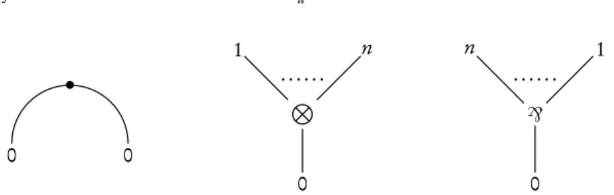
Chapter 2 2.: The components of a proof net: ax.-link, ⊗n-link and `n-link. . . 25

2.2 Unfolding a MLL_uproof net. . . 27

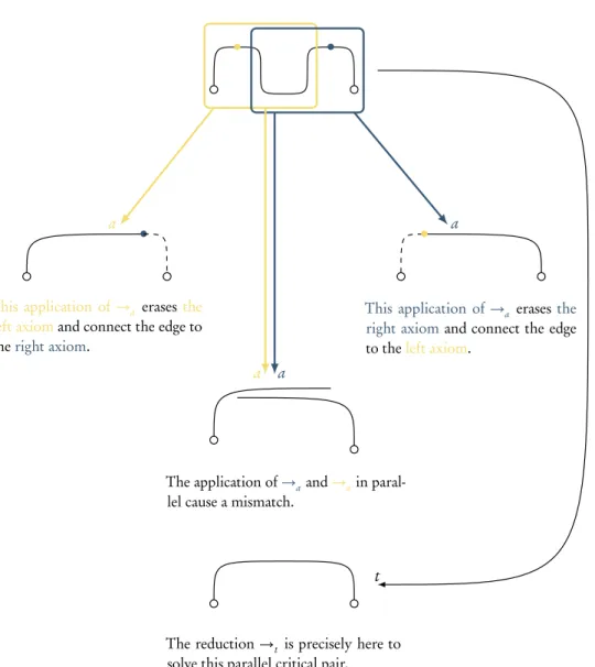
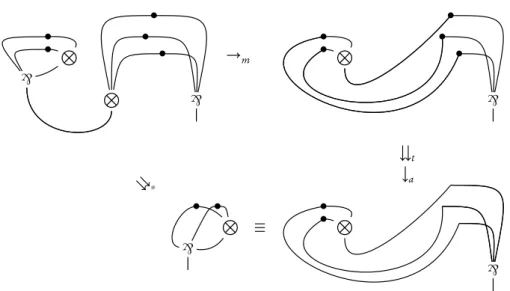
2.3 Cut-elimination in parallel: t-, a- and m-reductions . . . 27

2.4 An obstacle to cut-elimination in parallel . . . 29

2.5 Adding or removing a crossing: how negation works . . . 3:

2.6 The conditional, the core of the computation. . . 3:

2.7 Branching variables on a Boolean proof net and evaluating it. . . 32

2.8 Pieces of Proof Circuits . . . 33

2.9 The improvement of “built-in” composition. . . 36

2.:0 Contractibility rules: relabelling and contracting a pseudo net. . . 37

2.:: Composing two proof circuits. . . 4:

2.:2 The simulation of a Boolean proof net by a Boolean circuit. . . 44

2.:3 The access to the input in an input normal form ATM. . . 46

2.:4 The translation from Alternating Turing Machines to proof circuits . . . 48

2.:5 How a value is guessed by an Alternating Turing Machine . . . 49

2.:6 A shorthand for the “guess and check” routine . . . 50

2.:7 A function to compute the value carried by an edge. . . 52

Chapter 3 3.: The derivation of a unary integer, without contraction rule. . . 6:

3.2 Unaries as proof net . . . 62

3.3 Unaries as proof net, with contraction . . . 64

3.4 Binary integers as derivations . . . 70

3.5 The binary sequence ⋆001011⋆ as a proof net and as a circular string. . . 7:

3.6 Some explanations about the matricial representation of a binary word. . . 73

3.7 Representation of the main morphisms defined in the proof of Lemma 3.5.:. . . 86

3.8 A representation of the computation of an operator . . . 87 xi

Chapter 4

4.: How a KUM sorts integers. . . 97

4.2 How to simulate Turing Machines with Finite Automata . . . :05

4.3 The operators encoding the forward and backward move instructions. . . ::5

4.4 The operators encoding rejection. . . ::7

Appendix A A.: Dependency of the algebraic structures . . . :27

Appendix B B.: The transition relation that decides STConnComp . . . :43

Notations

The entries are divided between Complexity, Logic and Mathematics. Although some symbols are used in different ways, the context should always makes clear which denotation we have in mind.

We deal with classes of complexity separately, below this table of notations.

Complexity

ATM Alternating Turing Machine. . . .6

B_b A set of (bounded) Boolean functions (a basis) . . . .22

B_u A set of (unbounded) Boolean functions (a basis) . . . .₂₂

C Family of Boolean circuit . . . .23

C, Cn Boolean circuits . . . .22

CM The set of pseudo-configurations of a PM(p) M. . . .:08

DFA(k) Set of deterministic Multi-Head Finite Automaton with k heads . . . .99

DPM(p) The set of deterministic pointer machines with p pointers . . . .:08

G_{M (x)} Computation graph of an ATM M on input x . . . .8

G_{M ,n} Computation graph of an ATM M on input of size n . . . .46

Ò (·) Translation from families of computation graphs to proof circuit families . . . .47

L_{(M )} Language accepted by a machine M . . . .7

L_DC(C) Direct Connection Language of a family of Boolean circuits C . . . .23

LDC(P) Direct Connection Language of a family of Boolean proof nets P . . . .32

[not a] Any symbol of the alphabet except a . . . .99

NFA(k) Set of Non-Deterministic Multi-Head Finite Automaton with k heads. . . .98

NPM(p) The set of non-deterministic pointer machines with p pointers . . . .:08

O “Big O” asymptotic notation . . . .5 xiii

PM(p) The set of (deterministic and non-deterministic) pointer machines with p pointers .:08

P_+,1 Set of boolean observations of 1-norm ¶ 1 . . . .83

P₊ Set of boolean observations . . . .83

P_¾0 Set of positive observations . . . .83

Q↑ _{Extended set of states . . . .::0}

♯H Distance between  and the bit currently read by the head H . . . .99

σ Transition relation of a NDPM. . . .98

|x| The size of x . . . .5

⋆ First and last bit of a circular binary word. . . .69

 Left end-marker on the input tape of a FA. . . .98

à Right end-marker on the input tape of a FA . . . .98

⊢M (x) The transition relation between configurations in an ATM M on input x . . . .7

< 1y_{,g , p, b> The tuples used to describe a proof net. . . .32}

{X } Language decided by the set of observations X . . . .82

Logic

A[B/D] The substitution of every occurrence of B by D in A. . . .24

A[D] The substitution of every occurrence of α by D in A. . . .24

α Literal (or atom). . . .:3

−→ A, (resp.←−A) The ordered sequence of formulae A1, . . . ,An, (resp. An, . . . ,A1) . . . .24

⇒ The parallel evaluation of a proof net . . . .28

B The Boolean type of MLLu. . . .28

b₀, b1 Proof nets representing 0 and 1 in MLLu. . . .28

(·)⊥ _{Negation, or duality . . . .:3}

P Boolean proof net . . . .30

P A Boolean proof net familly . . . .₃₀

d (A) Depth of a MLL_uformula A. . . .25

⊢ Γ A sequent, Γ being a multiset of formulae. . . .:3

⇒ Classical implication . . . .:2

⊸ Linear implication . . . .:3

MLL_u Multiplicative Linear Logic . . . .24

• An axiom link, in a proof net . . . .25

! The “of course” modality . . . .:3

` The multiplicative disjunction (“par”) . . . ._:3

P Piece of a proof circuit . . . .33

Pb Set of pieces of bounded fan-in . . . .35

Pu Set of pieces of unbounded fan-in . . . .35

P_,Q Proof nets of MLL_u. . . .25

π A proof, in the sequent presentation . . . .:4

⊗ The multiplicative conjunction (“tensor”) . . . .:3

? The “why not” modality . . . .:3

Mathematics

α Action of a group. . . .:37

| · | Absolute value . . . .:32

B_(H) Banach algebra of continuous mapping over H . . . .:3:

det(M) Determinant of a matrix M. . . .:34

d Distance function . . . .:26

δi j Kronecker delta . . . .:26

∼M Murray and von Neumann equivalence over the von Neumann algebraM. . . .:33

F Field. . . .:27

⌊·⌋ Floor function . . . .:02

G Group . . . .:27

H Hilbert space. . . .:30

M[i, j ] Element in the ith row and j th column of M . . . .:34

M_n,m(F ) Matrix of dimensions n × m with coefficients in the field F . . . .:34

M von Neumann algebra . . . .:3:

M_{⋊ G} Crossed product of a von Neumann algebraMwith a group G . . . .:37

k·kk1 The 1-norm . . . .82

πk,i Projection of dimension (k + 1) × (k + 1) . . . .74

Π₍M) Set of projections of a von Neumann algebraM. . . .:33

P_fin(S) Set of finite subsets of S . . . .6

R The II₁hyperfinite factor. . . .:34

(·)∗ _{Involution . . . .:30}

S (S) Permutation group of S . . . .:28

S Group of all finite permutations over N . . . .:28

sgn(σ) Signature of a permutation σ . . . .:28

⊗ Tensor product . . . .:33

T Topology (over a set) . . . .:3:

tr(M) Trace of a matrix M. . . .:34

Tr(M_n) Normalised trace of a n × n matrix M_n. . . .:35

G Underlying set of the algebraic structure G . . . .:27

V Vector space . . . .:28

See referenced pages for formal definitions.

We are going to use several classes of complexity, some of them classical, some of them being introduced in this work (in a yellow rectangle in the figure below). The following pictures describe the situation at the end of our work. Some equalities and inclusions are classical, but we will in the course of this work give at least ideas of proofs for every of them.

For all i > 1,5_{we have at the end ofChapter 2}6_{the following situation:}

5_{Even if those bounds are going to be sharpened, we prefer to give our results in all generality at this point.} 6_Seeerrata.

Definition :.:.:2andDefinition 2.:.5

Definition 2.2.8

NCi ⊆ bPCCi ⊆ ACi _{⊆ PCC}i _{⊆ mBN}i

Chapter 3andChapter 4will define and prove properties about the following classes: Definition 3.4.7 Definition :.:.:: Definition 4.2.: Definition 4.3.: {P+} = {P¶0} = co-NL = NL = NFA = NPM {P+,1} = co-L = L = DFA = DPM

We are also going to introduce STA(∗,∗,∗) (Definition :.:.7) as a convenient notation to express any of these classes.

Preface

T

his work is somehow two-sided, for it studies two models of computation —and the implicit characterization of complexity classes that comes with— that share the same tool and the same aim, but are not directly related. The tool —mainly proof theory, and more precisely Linear Logic— and aim —to contribute to the complexity theory— are presented inChapter :. TheSection :.3presents some of the previous attempts to link those two fields.

The first model —presented inChapter 2— is related to the simulation of efficient computation in parallel with Boolean proof nets. It introduces proof circuits as an innovative way of understanding the work led by Terui. It sharpens the characterization of some complexity classes, and provides new evidence that this model is pertinent by linking it to the more classical Turing Machines. This chapter is —almost— self-contained and a gentle introduction to some important concepts.

The second model is presented inChapter 3, it develops a new world where logic is dynamically built from von Neumann algebras. We tried to ease the reading of this quite technical material by pushing slowly the constructions and taking time to explain some of the choices we made. We finish this first part by showing how complex our object is from a complexity point of view.

Chapter 4gently presents some “pointer machines” before defining a model that is proven adapted to be simulated by the model ofChapter 3. It recollects some historical variation to help the reader to understand the framework we are working with.

We made the choice to put aside inAppendix Athe introduction of the mathematical tools needed to understand the most advanced elements ofChapter 3. This disposition could disturb the reader by forcing him/her to go back and forth betweenChapter 3and this appendix. Yet, those tools should remains only tools, for they are not what is at stake here, and we tried to go as rapidly as possible to the point without getting too technical.

TheAppendix Bgives an alternate proof of a statement ofChapter 4. It is somehow more algorith-mic, for two problems are proved solvable by machines that are actually described. It is worth reading for it get some insight on pointer computation, and by extension on log-space reduction.

The picture that follows presents some of the dependencies between the different parts of this work.

m

:.:–Computational Complexity Theory :.2–Linear Logic

A–Operator Algebras Preliminaries :.3–Previous Gateways between Linear Logic and Complexity

2–Proof circuits

From

3.:–Complexity and Geometry of Interaction to

3.4–How to Compute

3.5–Nilpotency Can Be Decided With Logarithmic Space

From

4.:–JAGs and PURPLE: on the limitations of pebbles and pure pointers to

4.2–Finite Automata and L

4.3–Non-Deterministic Pointer Machines and

4.4–Simulation of Pointer Machines by Operator Algebra

Introduction

L

ogicis so tightly bound to computer science that the sonship is somehow reversed: computers, through programming languages, now teach us how reasoning can be algorithmically represented. We learnt how to modelise the cost of solving a problem, answering a question mathematically pre-sented. And yet Logic, thanks to the proof-as-program correspondence, still has a lot to say about this modelisation.

The first cost models that were developed on abstract machines discriminate between the “reason-able” models of computation and the one that are not. Of course, they could not foresee the inherent complexity of solving a precise problem: one had to actually run the program to observe the resources it needs to obtain a result. Some important problems, in a way equivalent to any other “as complex” problem, were defined and were taken as representative of the power of some complexity classes.

The Implicit Computational Complexity approach reversed this dependency, by defining frame-works where any algorithm that could be expressed was “pre-bounded”. Among the approaches devel-oped stands Linear Logic, and among the classes “captured” stands P, the class of “tractable” problems. This class drew a large part of the attention because of the challenge its separation from the other classes represents.

There is no reason to stick to that class, for Linear Logic has at its disposal numerous tools to simulate other ways of computing. Modalities —the salt of Linear Logic— were proven fruitful to handle the polynomial time complexity, but there are numerous other built-in mechanisms to cope with the complexity.

This work presents two innovative ways to represent non-deterministic and parallel computation with Linear Logic. They were not invented by the author, but by Terui and by Girard, respectively in 2004 and in 20:2. Those approaches have some elements in common, at least a part of the tools and the aims, and they are two natural extensions of a tradition of bridging the gaps between Linear Logic and complexity. Still, they are largely unexplored, excepted for two works led by Mogbil and Rahli, and except of Seiller’s PhD Thesis.

This work may be hard to get through, for it mixes three fields of research: complexity theory, Linear Logic, and a mathematical framework known as Geometry of Interaction. We tried to ease the presentation by developing some examples and by taking some time to discuss the general shape of the construction as well as some details. May this work ease the understanding of those two exciting approaches.

CHAPTER

:

Historical and Technical Preliminaries

T

hischapter will set up most of the elements needed to understand the rest of this work. A strict minimal knowledge on set theory and graph theory is required to grasp some definitions, but apart from that everything should be quite self-explanatory. However, we do not always take the time to introduce gently the notions and go straight to the point, but many references are provided.

This work takes place in the complexity area, a subject that mix theoretical computer science and mathematics, and tries to classify computational problems by their inherent complexity. This was historically done by showing off algorithms that run on abstract machines, where every operation is endowed with a cost, and by studying the overall cost of the computation. To be pertinent, this consumption of resources is expressed relatively to the size of the input by a function that does not have to be precise: we ignore the constant factors and the lower order terms to focus on a larger magnitude.

Later on came the Implicit Computational Complexity, that describe complexity classes without explicit reference to a machine model and to bounds. It massively uses mathematical logic to define programming language tools —like type-systems – that enforce resource bounds on the programs. Among the techniques developed, one could mention

◦ Recursion Theory, which studies the class characterized by restricting the primitive recursion schema.: ◦ Model Theory, which characterizes complexity classes by the kind of logic needed to express the languages in them. It is also known as Descriptive complexity, and we refer to Immerman [77] for a

clear and self-contained presentation.

◦ Proof Theory, which uses the Curry-Howard correspondence to match up execution of a program and normalisation of a proof.

This latter way of characterizing complexity classes by implicit means is a major accomplishment of the cross-breeding of Logic and computer science. We will in the third section gives some examples of the previous works led onto that direction, but we will first present its two components: computational complexity theory, and a special kind of logic, Linear Logic.

:_{The seminal work was made by Leivant, but one could with benefits look to a clear and proper re-statement of his results by}

Dal Lago, Martini, and Zorzi [34].

:

.: Computational Complexity Theory

A short and yet efficient introduction to the theory of complexity can be found in the chapters “Basic notions in computational complexity” written by Jiang, Li, and Ravikumar [82] and published in a

classical handbook[6]. In the same book, the two chapters written by Allender, Loui, and Regan

[:,2], “Complexity Classes” and “Reducibility and Completeness” synthesise all the results that will be

used in this section. The handbook of Papadimitriou [:::] is often refereed to as “the” handbook for a

nice and complete introduction to this theory: its unique style allows to read it as a novel, and to grasp the tools one after the other, but for the very same reason it is hard to look for a precise information in it. The reader searching for a precise definition or a theorem should probably rather refer to the textbooks of Greenlaw, Hoover, and Ruzzo [65], and Arora and Barak [4].

Complexity and models of computation

This section will quickly try to present what a “reasonable” model of computation is, what is at stake when we take parallel models of computation, and gives hints toward the specificities of subpolynomial classes of complexity. It borrows some elements from van Emde Boas [:32], whose preliminary

chapter is clear and concise.

To study complexity in an “explicit” framework, one needs a machine model and a cost model. A machine model is a class of similar structures, described set-theoretically as tuples most of the time, endowed with a program, or finite control, and a definition of how computation is actually performed with a machine of that model. The cost model fixes the cost of the basic operations, allowing to measure the resources (most of the time understood as time and space) needed to process an input.

Two fundamentals of this theory is that something is “algorithmically computable” iff it is com-putable by a Turing Machine (Church–Turing thesis), and that taking the Turing Machine or another “reasonable” model of computation does not really matter, this is the invariance thesis:

Invariance Thesis. “Reasonable” machines can simulate each other within a polynomially bounded over-head in time and a constant-factor overover-head in space.

Of course, what is a simulation needs to be define.

Definition :.:.: (Simulation). Given two machines models M and M′_{, we say that M}′ _{simulates M}

with time (resp. space) overhead f (n) if there exists two functions c and s such that, for every machine Mi in M:

◦ for all input x of M , c(x) is the translation of x in the setting of M′_;

◦ Mi(x)halts iff Ms(i)′ (c(x))halts, and Mi(x)accepts iff Ms(i)′ (c(x))accepts2;

◦ if t(|x|) is the time (space) bound needed by Mi for processing x, then the time (resp. space) required

by M′

s(i)for processing c(x) is bounded by f (t(|x|)) ;

If the time overhead function f is linear, the simulation is said to be real-time.

2_{Where M}

Something is missing in this “definition”: what are the resources needed to compute s and c? It would be meaningless to provide more computational power to compute M′

s(i) than what Ms(i)′ can

actually provide: we could as well have computed the output directly! In other words, if the machine used to process c and s is strictly more powerful than M′

s(i), we cannot extract any knowledge about M′.

In the following, we need to be careful about the cost of those simulations.

We will tend to keep the word simulation for the case where c and s are computed by a machine of M′ _{itself: in other word, provided a description of M}

i, the machine Mi′ will by itself “acts as Mi”,

without external intervention. If a third machine model M′′_{, given the description of M}

i and x, outputs

the description of M′

s(i)and c(x), we will speak of a translation.

Notice that f takes as input |x| the size of the input, for we measure the resources needed by the computation relatively to the size of the input. This function should be proper,3 _{i.e. it should respect} some basic properties, but we won’t take that parameter into account, for we will use only the proper functions below:

Polynomial i.e. there exists c, d∈ N∗_{such that f (|x|) is bounded by c × (|x|}d_).

Constant i.e. there exists c∈ N∗_{such that f (|x|) is bounded by c × |x|.}

(Binary) Logarithm i.e. there exists c∈ N∗_{such that f (|x|) is bounded by c × (log(|x|)).}

Poly-logarithmic i.e. there exists c, i∈ N∗_{such that f (|x|) is bounded by c × (log}i₍

|x|)).

We will use the “big O” asymptotic notation, i.e. we write that g =O(f )iff ∃k ∈ N∗such that ∀x, g(x) ¶ k × f (x). So if f is a polynomial (resp. the constant function, the logarithm, a poly-logarithm), we will sometimes write nO(1)_{(reps. O(1),O(log),O(log}i_{)) or even more simply poly}

(resp. 1, log, logi_{), without any reference to the size of the input.}

This notation is a bit counter-intuitive, because despite the equal sign, it is not symmetric:O(x) =

O(x2_{)is true butO(x}2_{) =O(x)is not. As Sipser [:24, p. 277] writes it, “[t]he big-O interacts with}

logarithms in a particular way”: the changing of the base of the logarithm affects the complexity only by a constant factor, so we may simply ignore it and we will consider that the logarithmic function is always in base 2. We will use in the course of this work some classical identities, but maybe it is worth remarking that as n = 2log(n)_{, for all d ∈ N, n}d ₌₂d log(n)_{and so 2}(log(n))O₍₁₎

=nO(1)_{. We can also remark}

that as log(nd_{) =d log(n), log(n}O(1)_{) =O(log(n)). This will be more or less the only two equalities we}

are going to use.

We will focus here on the subpolynomial world, that is to say the machines that use less resources than polynomial time. This world is less studied than the polynomial word, as the “reasonable” compu-tation is quite limited in it, but a fruitful approach often used is to look toward parallel compucompu-tation. This world also have a kind of invariance thesis to define what is a reasonable model:

Parallel Computation Thesis. Whatever can be solved in polynomially bounded space on a reasonable sequential machine model can be solved in polynomially bounded time on a reasonable parallel machine, and vice versa.

This thesis was first formulated by Goldschlager [64], and by Chandra, Kozen, and

Stock-meyer [24] quite simultaneously. The first one stated that “Time-bounded parallel machines are

polynomially related to space-bounded computers” by trying to “capture mathematically this intuitive

notion of parallel computation, much in the same spirit that ‘Church’s thesis’ captures the notion of effective computation.” Chandra, Kozen, and Stockmeyer, on their way, defined Alternating Turing Machine and proved that “an alternating Turing machine is, to within a polynomial, among the most powerful types of parallel machines”.

Alternating Turing Machines are also the most general version of the most well-known model, Turing Machines, so it is quite natural to take them as the reference, as the basic model. We should

make one last remark concerning this parallel world: time is sometimes refereed to as the depth, i.e. the maximal number of intermediate steps needed ; and space is taken to be the size, i.e. the number of processors needed to perform the computation. This will be the case with the Boolean circuits and the proof circuits, defined inChapter 2.

Alternating Turing Machine

This model of computation is really handy, for it will allow us to define at the same time parallel and sequential computing, and it has a characterization of every complexity class we will use in the following. The following definition borrows some elements of the clear presentation of Vollmer [:35,

p. 53].

Definition :.:.2 (ATM, Chandra, Kozen, and Stockmeyer [24]). An Alternating Turing Machine

(ATM) M with k ∈ N∗_{tapes is a 5-tuple}

M = (Q, Σ,δ, q₀,g ) with

◦ Q a finite set of states, ◦ Σ an alphabet,4

◦ δ : (Q × Σk+1_{× N}k+1_)→P

fin(Q× Σk× {−1,0,+1}k+1)the transition relation,

◦ q0∈ Q the initial state,

◦ and g : Q → {∀,∃,0,1} the state type function.

This definition does not explain how one can actually perform a computation with ATMs, and we will quickly expose those —very classical— mechanism right after we introduce some nomenclature.

The input is written on the input tape, and the head that scans it is read-only. The other k heads are read-write, and each one of them work on a dedicated tape. A configuration α of M is an element of Q× (Σ∗₎k_{× N}k+1_{that entirely describe the current situation. It reflects the current state, the content}

of the k working tapes and the position of the k + 1 heads, as a “snapshot” from where it is possible to resume the computation, provided that we know the input and the transition relation.

The initial configuration α0of M is when the entry is written on the input tape, the k working

tapes are blank,5_{the k + 1 heads are on the first cell of their tape, and the state is q}

0.

A state q ∈ Q —and by extension a configuration whose state is q— is said to be universal (resp. existential, rejecting, accepting) if g (q) =∀ (resp. ∃, 0, 1). A state q ∈ Q —and a configuration whose state is q— is final if ∀a0, . . . ,ak∈ Σ, δ(q,a0, . . . ,ak) =;. This condition is equivalent to g(q) ∈ {0,1}.

4_{One should precise that every tape is divided into cells and that every letter of the alphabet need exactly one cell to be written.} 5_{Usually a special “blank” symbol ♭ is written on every cell, but it works as well to take any symbol of the alphabet.}

Suppose that M is working on input x ≡ x1. . .xn(we denote this situation with M(x)) and that at a

certain point, M is in configuration

α = (q, w1, . . . ,wk,n0, . . . ,nk)

where w_i≡ wi,1. . .wi,li for 1 ¶ i ¶ k. Suppose that δ(q, xn0,w1,n1, . . . ,wk,nk)contains (possibly among others) the tuple (q’,a1, . . . ,ak,X0, . . . ,Xk), where a1, . . . ,ak∈ Σ and X0, . . . ,Xk∈ {−1,0,+1}. Then

β = (q’, w1′, . . . ,wk′,n0′, . . . ,n′k)

is a successor configuration of α, where for 1 ¶ i ¶ k, w′

i is obtained from wi as follow: replace the nith

letter by ai, and to cover the case where the head moves to the left or right out of the word by prefixing

or suffixing the blank symbol ♭ ; and for 0 ¶ i ¶ k, let n′

i=ni+Xi, if ni+Xi¾ 0, otherwise we leave

n′ i=ni.

That β is such a successor configuration of α (and respectively that α is a predecessor of β) is denoted by α ⊢M (x)β, or if M and x are clear from the context by α ⊢ β. As usual, ⊢∗is the reflexive transitive

closure of ⊢. Observe that a final configuration has no successor and that the initial configuration has no predecessor.

A computation path of length n in M(x) is a string α1, . . . ,αn such that α1⊢M (x). . . ⊢M (x)αn. We say

that M(x) has an infinite computation path if for every n ∈ N there exists a computation path of length n. A computation path α1, . . . ,αnis cyclic if α1=αn.

We should be more rigorous and define the ATM to be a 6-tuple with k —the number of tapes— to be a parameter. But thanks to some classical theorems, we know that the number of tapes does not really matter, even if we have complexity concern: an Alternating Turing Machine with k tapes can reasonably be simulated with an Alternating Turing Machine with 3 tapes, one for the entry, one working tape, and one tape to write down the output.

In fact, we won’t even bother taking into account the output tape in most of the case, for our Alternating Turing Machines will only decide, i.e. accept or reject an input, as the following definition explains.

Definition :.:.3 (Accepted word). We define a labelling l from the configurations of M (x) to{0,1}: a configuration α of M(x) is labelled with 1 iff

◦ g(α) = 1, or

◦ g(α) = ∀ and for every configuration β such that α ⊢ β, l (β) = 1, or ◦ g(α) = ∃ and there exists a configuration β such that α ⊢ β and l (β) = 1.

We can recursively label every configuration of M(x) with l. As soon as the initial configuration of Mhas been labelled, we can stop the procedure and leave some configuration unlabelled.

A word x ∈ Σ∗_{is said to be accepted by M if the initial configuration of M(x) is labelled with 1. We}

setL(M ) ={x ∈ Σ∗_{| M accepts x}.}

Once the computation is done,6_{that is to say when the initial configuration may be labelled, we can} know what are the resources consumed by the processing of the input. We define three costs models on our ATMs.

6_{This is precisely what differentiate implicit and explicit computational complexity. Here, we have to perform the computation}

Definition :.:.4 (Bounds on ATM). Given M an ATM and s, t and a three functions, we say that M is space- (resp. time-, alternation-) bounded by s (resp. t, a) if for every input x of size |x|,

at every moment, at mostO(s(|x|)) cells of the working tapes are left non-blank,7 every computation path is of length at mostO_{(t (|x|)),}

in every computation path, the number of times an existential configuration has for successor an uni-versal configuration plus the number of times an uniuni-versal configuration has for successor an existential configuration is at mostO_(a(|x|)).

Note that if M is space-bounded by s then given an input x the number of configurations of M is at most 2O(s(|x|))_{: M(x) can have Card(Q) different states, the working tapes can contains k × Card(Σ)}s(|x|)

different words of length at most s(|x|), the head on the input tape can be in |x| different places and the k heads can be in k × s(|x|) different positions. To sum up, M(x) can only have Card(Q) × (k × Card(Σ)s(|x|)_{)× (|x|) × (k × s(|x|)) different configurations. As all those value except |x| are given with}

M, so we know there exists a d such that M(x) has less that 2d×s(|x|)_{different configurations.}

Moreover, if M is bounded in time by t, then M is bounded in alternation by t, for M cannot “alternate more than it computes”.

If all the configurations are existential (resp. universal), we say that M is a non-deterministic (resp. universally non-deterministic) Turing Machine. If the transition relation δ is functional, M is said to be a deterministic Turing Machine.

The rest of this subsection will define some other important notions like problems, reductions or complexity classes. We should dwell however on the links between Alternating Turing Machines, graphs and parallel complexity. It will be proven very useful in the rest of this thesis.

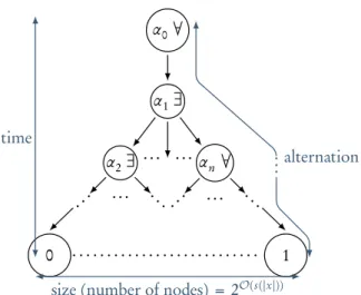
Definition :.:.5 (Computation graph, inspired by Vollmer [:35, p. 54]). Given an ATM M and

an input x ≡ x1. . .xn, a computation graph GM (x)is a finite acyclic directed graph whose nodes are

configurations of M, built as follow: ◦ Its roots is the initial configuration of M ,

◦ if α ∈ GM (x)and α ⊢ β, then β ∈ GM (x)and there is an edge from α to β,

A node in GM (x)is a sink if the associated configuration is final.

The computation graph associated to M on input x, GM (x), is of depth8O(t (|x|)) if M is bounded

in time by t. If M is bounded in space by s, the number of configurations of M is bounded by 2O(s(|x|))

and so is the number of nodes of G_{M (x)}. Note also that if M is deterministic, G_{M (x)}is a linear graph. To get a better insight on this construction, one may refer toFigure :.:where the example of a computation graph is sketched.

To determine from a computation graph if the course of computation described leads to acceptance of rejection, we simply have to label every node following the procedure described inDefinition :.:.3.

7_{The entry tape does not count in the measure of the space needed to perform a computation. We dwell on that point for it}

would make no sense to speak of a computation using a logarithmic amount of space in the size of the input elsewhere: one would not event have the space to write down the input! This is one of the “log-space computation oddities”, more are to come.

8_{The depth of G}

α0∀ α1∃ α2∃ . . . . . . . . . _α n∀ . . . ... ... ... ... 0 1 time alternation .. .

size (number of nodes) = 2O(s(|x|))

Figure :.:: The computation graph of an ATM

InSection 2.4, we will define ATMs in input normal forms (Definition 2.4.:) and use this crucial notion to define family of computation graphs (Definition 2.4.2).

This definition as the others use some classical theorems without stating them. For instance, the fact that a computational graph is finite and acyclic comes from two reasonable modifications that one can perform on any ATM. We can always add a clock to our ATMs, and forgive any transition such that α ⊢ β ⊢∗_{α, i.e. to prevent any loop in our program. Notice also that we did not bother to define}

negative states for our ATMs, for it was proven in the very first paper on this topic [24, Theorem 2.5,

p. :20] that those states did not bring any computational advantage.

We will also use the following classical modifications: we can always take the alphabet Σ to be {0,1} and the number of working tapes k to be 1. This has some minor consequences on the complexity of our object, but stay within the realm of “reasonable” modifications, i.e. does not modify the complexity classes characterized.

Problems and complexity classes

Definition :.:.6 ((Decision) Problem). A problem P is a subset of N. If there exists M an ATM, such that for all x ∈ N, M(x) accepts iff x ∈ P, we say that M decides P. We will sometimes say in this case that P is the language of M, i.e. we defineL(M ) ={n ∈ N | M (x) accepts}.

Definition :.:.7 (STA(∗,∗,∗)9_{). Given s, t and a three functions, we define the complexity class} STA(s, t, a)to be the set of problems P such that for every of them there exists an ATM bounded in space by s, in time by t and in alternation by a that decides it.

If one of the function is not specified, there is no bound on that parameter and we write ∗, and if —in the case of alternation— we allow only ∃ (resp. ∀), we write ∃ (resp. ∀) in the corresponding field.

If M is deterministic, we write d in the alternation field.

Decisions problems are not sufficient to define everything we need, for instance because the sim-ulation of theInvariance Thesisneeds to process functions. Roughly, we say that a function f is

computable in C if a machine with corresponding bounds can for all x ∈ N write on a dedicated tape (“the output tape”) f (x). Note that the space needed to write down this output may not be taken into account when measuring space bound, for we can consider it is a write-only tape. This is one of the reasons composition is so tricky in the log-space bounded word: if we compose two log-space bounded machines M and M′_{, the output-tape of M becomes one of the working tape of M ◦ M}′_{, and so M ◦ M}′

does not respect any more the log-space bound.

This also force us to trick the classical definition of “reductions”, that are the equivalent of simula-tion between machine models when applied to problems:

Definition :.:.8 (Reduction). Given two problems P and P’, we say that P reduces to P’ with a C-reduction and we write P ¶CP’ iff there exists a function f computable in C such that for all x, x∈ P

iff f (x) ∈ P’.

There is a whole galaxy of papers studying what a reduction exactly is, for one should be really careful about the resources needed to process it. We refer to any classical textbook for an introduction to this notion, but we define anyhow log-space reduction for it will be useful.

Definition :.:.9 (log-space reduction). A function f :{0,1}∗_{→ {0,1}}∗_is:0_{said to be implicitly log-space} computableif there exists a deterministic Turing Machine with a log-space bound that accepts < x, i > iff the ith bit of f (x) is 1, and that rejects elsewhere.

A problem P is log-space reducible to a problem P’ if there exists a function f that is implicitly log-space computable and x ∈ P iff f (x) ∈ P’.

Reduction should always be defined accordingly to the resources consumed, but in the following we will always suppose that the “handy” reduction is taken, i.e. the one that uses the less (or supposedly less) computational power. An other crucial notion for complexity theory is the notion of complete problem of a complexity class: this notion somehow captures a “representative problem”, it helps to get an intuitive understanding of what a complexity class is capable of.

Definition :.:.:0 (C-complete problem). A problem P is C-complete (under a C′_{-reduction) if}

◦ P ∈ C

◦ For all P’ ∈ C, P’ ¶C′P with C′⊆ C.

If P entails only the second condition, P is said to be C-hard.

We can now define some classical complexity classes, first the sequential complexity classes, the one that can be defined without really taking profit of alternation:

Definition :.:.:: (Complexity classes).

L = STA(log,∗,d) (:.:)

NL = STA(log,∗,∃) (:.2)

co-NL = STA(log,∗,∀) (:.3)

P = STA(log,∗,∗) = STA(∗,poly,d) (:.4)

We introduced here the complementary of a complexity class, namely co-NL. Let P be a problem, PComp is{n ∈ N | n /∈ P}. For any complexity class C, co-C denotes the class {PComp | P ∈ C}. If a problem P ∈ C can be decided with a deterministic machine, it is trivial that PComp can be decided with the same resources, it is sufficient to inverse acceptance and rejection, and so C = co-C.

We chose here to define the classical parallel classes of complexity AC and NC in terms of Alternat-ing TurAlternat-ing Machines, the other definition in terms of Boolean circuits beAlternat-ing postponed toDefinition 2.:.5. The correspondence between those two definitions is a mix of classical results [:5, p. :4] (eq. (:.6)), [25],

[:23], [::5] (eq. (:.8)).

Definition :.:.:2 (Alternation and parallel complexity classes). For all i ¾ 1

AC0=STA(∗,log,1) (:.5) NC1=STA(∗,log,∗) (:.6) ACi=STA(log,∗,logi) (:.7) NCi=STA(log, logi,∗) (:.8) We define ∪iACi=ACand ∪iNCi=NC. Theorem :.:.: (Hierarchy). AC0( NC1⊆ L ⊆ NL = co-NL ⊆ AC1⊆ NC2⊆ ... ⊆ AC = NC ⊆ P For all i ∈ N, ACi

⊆ NCi+1is quite evident, for a bound of logi+1_{on time is sufficient to perform}

at least logi_{alternations. That AC}0

( NC1is a major result of Furst, Saxe, and Sipser [44] and made

the Boolean circuits gain a lot of attractiveness, for separation results are quite rare!

The proof of NL ⊆ NC2_{is rather nice, and one may easily find a clear explanation of it [}

:35, p. 4:,

Theorem 2.9]: a matrix whose dimension is the number of configurations of a log-space Turing Machine is built in constant depth,::_{and a circuit of depth log}2_{computes its transitive closure in parallel.}

At last, co-NL = NL is a major result of Immerman [78]. It was proven by showing how a

log-space bounded Turing Machine could build the computation graph of another log-space bounded Turing Machine and parse it to determine if there is a path from the initial configuration to an accept-ing configuration. That co-L = L is trivial, since every deterministic complexity class is closed by complementation.

Turing Machines indeed share a lot with graphs, especially when they are log-space bounded. We illustrate that point with two (decision) problems that we will use later on. They both are linked to connectivity in a graph, and can be also refereed to as “reachability” or “maze-problem”. Numerous papers are devoted to list the problems complete for a class, we can cite among them Jenner, Lange, and McKenzie [8:] and Jones, Lien, and Laaser [85].

Problem A: Undirected Source-Target Connectivity (USTConn)

Input: An undirected graph G = (V, E) and two vertices s, t ∈ E

Output: Yes if s and t in the same connected component in G, i.e. if there is a path from s to t.

::_{That is to say with a family of constant-depth unbounded Boolean circuit. It might just be understand for the time being as}

Reingold[::4] proved that USTConn is L-complete (hardness was proved by Cook and

McKen-zie[28]). We will use inChapter 2its bounded variant, where G is of degree at most n, USTConn₂.

We will also use inAppendix Ba small variant of its complementary, where s and t are not parameters, but always the first and the last nodes of V .

This problem also exists in a directed fashion:

Problem B: (Directed) Source-Target Connectivity (STConn ) Input: A directed graph G = (V,A) and two arcs s, t ∈ A Output: Yes if there a path from s to t in G.

STConn is NL-complete.

The proof that every NL-problem can be reduced to STConn is really interesting, for it links closely log-space computation and graphs.:2 _{Let P ∈ NL, there exists non-deterministic log-space bounded} Turing Machine M that decides it (otherwise there would be no evidence that P ∈ NL). There exists a constant-depth boolean circuit that given n ∈ N and the description of M outputs GM (n)the

configura-tion graph of M. Then n ∈ P iff there is a path between the initial configuraconfigura-tion and a configuraconfigura-tion accepting in GM (n), a problem that is STConn.

:.2 Linear Logic

Linear Logic (LL) was invented by Girard[47] as a refinement of classical logic. Indeed, (classical)

logic is a pertinent tool to formalise “the science of mathematical reasoning”, but when we affirm that a property A entails a property B (A ⇒ B), we do not worry about the number of times A is needed to prove B. In other words, there is no need to take care of how resources are handled, since we are working with ideas that may be reproduced for free.

We just saw that if we have complexity concerns, one should pay attention to duplication and erasure, for it has a cost. The implication ⇒ superimposes in fact two operations that Linear Logic distinguishes: first, there is the linear implication A ⊸ B that has the meaning of “A has to be consumed once to produce B”, and the of course modality !A that has the meaning of “I can have as many copies (including 0) of A as I want”. Thus, the classical implication A ⇒ B is encoded as (!A) ⊸ B. From this first remark, numerous tracks were followed: we will begin by recalling the main ideas of Linear Logic, and then focus on proof nets before presenting the Geometry of Interaction (GoI) program.

The reference to study Linear Logic remains Proofs and Types[62], and the reader not used to this

subject could read with benefits the :0 pages of Appendix B, “What is Linear Logic?”, written by Lafont. For anyone who reads french, Joinet’s Habilitation à diriger les recherches[83] is an excellent

starting point to put Linear Logic into philosophical and historical perspective. The two volumes of Girard’s textbook [55, 56] were translated in English[58] and are the most complete technical

introduction to the subject.

Main concepts and rules

We will tend during the course of this work to dwell on the syntactical properties of Linear Logic, but we should however remark that some of its elements appeared first in Lambek [94]’s linguistic

considerations. Linear Logic is a world where we cannot duplicate, contract and erase occurrences

:2_{For a more advanced study of those links, one could have a look at the work led by Wigderson [:36] and to its important}

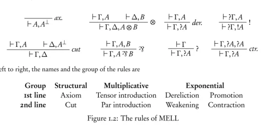
ax. ⊢ A,A⊥ ⊢ Γ ,A ⊢ ∆,B ⊗ ⊢ Γ ,∆,A⊗ B ⊢ Γ ,A der. ⊢ Γ ,?A ⊢ ?Γ ,A ! ⊢ ?Γ ,!A ⊢ Γ ,A ⊢ ∆,A⊥ cut ⊢ Γ ,∆ ⊢ Γ ,A,B <sub>`</sub> ⊢ Γ ,A` B ⊢ Γ _? ⊢ Γ ,?A ⊢ Γ ,?A,?A _ctr. ⊢ Γ ,?A

From left to right, the names and the group of the rules are

Group Structural Multiplicative Exponential :st line Axiom Tensor introduction Dereliction Promotion 2nd line Cut Par introduction Weakening Contraction

Figure :.2: The rules of MELL

of formula for free. This led to the division of classical logic:3_{into three fragments: additive, whose} rules are context-sensitive, multiplicative, whose rules are reversible, and exponential, which handles the modalities. The negation of a formula is encoded thanks to the linear negation ⊥_{, which is an}

involution.

We will only use the MELL fragment (without units),:4 _{i.e. the multiplicative and exponential} connectives, whose formula are, for α a literal (or atom, a variable taken for a countable set), using the inductive Backus Normal Form notation:

A :=α | α⊥ | A⊗ A | A` A | !A | ?A.

The ⊗ connective is called tensor, the ` connective is called par, ! and ? are respectively named of course (or bang) and why not. Dualities are defined with respect to De Morgan’s laws, that allows us to let the negation flows down to the literals:

(A⊗ B)⊥:= A⊥`<sub>B</sub>⊥ <sub>(A ` B)</sub>⊥_{:= A}⊥_{⊗ B}⊥ _(!A)⊥_{:= ?(A}⊥_{) (α}⊥₎⊥_{:= α} The connective ⊸ is defined as A ⊸ B ≡ (A⊥_{) `B. We let Γ and ∆ be two multisets of formulae, and}

for ⋄ ∈ {!,?}, if ∆ = A1, . . .An, we let ⋄∆ be ⋄A1, . . . ,⋄An.

We borrow from Mogbil [:06, p. 8] the following presentation of rules and proofs, which is

especially handy. A sequent ⊢ Γ is a multiset of formulae of MELL, the order of the occurrences of formula plays no role for the time being. We let S be the set of sequents of MELL. For n ¾ 0, a n-ary rule Rnwith n hypothesis and one conclusion is a n + 1 relation on S, i.e. R ⊆ Sn× S. The set of rules

of MELL is given inFigure :.2, where the principal formula is distinguished in the conclusion sequent. A proof of height 0 in MELL is the unary rule ax.. For n 6= 0, a proof of height h 6= 0 Dh is a subset of

(D_<h)n× Rnsuch that

◦ the set D<his the set of proofs of height strictly inferior to h, ◦ the n conclusions of the n proofs of D<h are the n premises of Rn,

◦ the conclusion of Dhis the conclusion of Rn.

:3_{For a complete presentation of the variations of Linear, Classical and Intuistionistic Logic, we refer for instance to Laurent}

[95].

:4_{In a nutshell, it is natural to associate to the multiplicative fragment a parallel handling of the resources, whereas the additive}

A sequent ⊢ Γ is derivable in MELL if it admits a proof, i.e. if there exists a proof π whose conclusion is ⊢ Γ . The η-expansion of a proof π is a proof π′_{of same conclusion where the axioms}

introduce only literals. Such a proof π′_{always exists, and it is unique. A proof π is α-equivalent}:5_{to a} proof π′_{if π}′_{can be obtained from π by replacing the occurrences of the literals in π.}

One of the fundamental theorem of logic is Gentzen’s Hauptsatz, or cut-elimination theorem, proved first by Gentzen [45]:6 _{for classical and intuitionistic logic. This theorem applies as well} to MELL, and we sometimes say that a system eliminates cuts if it entails this theorem:

Cut-elimination Theorem. For every proof π of⊢ Γ in MELL, there exists a proof π′_{of same conclusion}

that does not uses the rule cut.

The Curry-Howard-correspondence (a.k.a. the proof-as-program correspondence) tells us that the operation of rewriting a proof with cuts into a proof without cuts corresponds to the execution of a program written in λ-calculus. This link between computer programs and mathematical proofs justifies the use of Linear Logic as a typing system on programs, and by extension, its use as a tool to modelise complexity. Before studying in depth how this gateway was used, we still need to introduce two other key-concepts of Linear Logic: proof nets and Geometry of Interaction (GoI). They correspond respectively to the model we develop inChapter 2, and to the model we develop inChapter 3.

Proof Nets

Proof Nets are a parallel syntax to express proofs that get rid of some lumbering order in the application of rules. For instance, one should not feel the urge to distinguish between the following two proofs obtained from the same proof π:

.. . π ⊢ A,B,C , D _{`</sub> ⊢ A` B,C , D _{`</sub> ⊢ A` B,C ` D .. . π ⊢ A,B,C , D <sub>`} ⊢ A,B,C ` D <sub>`} ⊢ A` B,C ` D

It was also introduced by Girard[5:] and provoked numerous studies, and yet there is to our

knowledge no “classical definition”. The most accurate one can be found in Mogbil’s Habilitation à diriger les recherches [:06, Definition 2.::, p. ::], it defines proof nets as hyper-multigraphs.

We will present in details and massively use proof nets for an unbounded version of Multiplicative Linear Logic inChapter 2. So despite the tradition to present some drawing to introduce them, we will just express some global ideas and refer the reader toSection 2.:for a complete presentation. We will use them only as examples and hints toward a sharper understanding inChapter 3, and they do not appear inChapter 4.

A proof net is built inductively by associating to every rule ofFigure :.2a rule on drawings. We obtain by doing so a labeleld graph, where the nodes are endowed with a connective of MELL, and the edges represents sonships between occurrences of formulae. This parallel writing of the proofs gives a quotient on proofs that “reduces the syntactical noise” and by doing so let the proofs be more readable. Every derivation infers a proof net, and by applying some quotient on the different representations of the same proof net, a proof net may be inferred by several proofs.

:5_{We won’t define this notion precisely here, for it is very tedious to do so, as attested by the :st chapter of Krivine [92].} :6_{The interested reader may find a translation [46].}

One should remark that none of those rules is local in this setting, for there is always (except for the axiom rule) a constraint on the membership of the principal occurrences to the same context or to two different contexts, not to state the constraint on the presence of a modality. This is the drawback of this representation: the correctness of a proof is not tested locally any more, as opposed to any other syntactical system that existed in the history. We call pseudo nets the structures freely-generated, that is, such that we don’t know if there exists a proof that infers it. To determine whether a pseudo net is a proof net, we need a global criteria to test its “legacy”. Those criterion are called criterion of correctness and we refer once again to Mogbil’s work [:06, p. :6] for a complete list. We will use one

of them inTheorem 2.2.:.

We left aside the presentation of those (yet very important) tools to focus on a crucial point for the well understanding of this thesis. As we presented it, the sequents of MLL are not ordered. An order could be introduced thanks to a bit tedious notion of exchanges of occurrences of formulae, allowing us to keep track of their positions. It is handy not to take care of this aspect, but we are forced to re-introduce it when dealing with proof nets: suppose given a proof π of conclusion ⊢ ?A,?A,?A,B,B. The proof π can be completed as follows:

.. . π

⊢ ?A,?A,?A,B,B _ctr. ⊢ ?A,?A,B,B <sub>`</sub> ⊢ ?A,?A,B ` B

The question is: if we label the conclusion of π with ⊢ ?A1, ?A2, ?A3,B1,B2, what is the conclusion of

the previous proof? It could be any sequent among

⊢ ?A1, ?A2,B1`B2 ⊢ ?A1, ?A3,B1`B2 ⊢ ?A2, ?A3,B1`B2

⊢ ?A1, ?A2,B2`B1 ⊢ ?A1, ?A3,B2`B1 ⊢ ?A2, ?A3,B2`B1

In fact, by dealing with non-ordered sequents, we already introduced a first quotient on our proofs, which is not compatible with proof nets. Remark that it does not contradict the fact that proof nets quotient proofs, for we may for this example performs the contractions and the par-introduction in parallel.

But in the following, we will encode the truth-value of a boolean type in the order of the the premise of a par-rule (Definition 2.2.:). The principal formulae of the contractions will later on encode the value of a bit in a string (Section 3.3). This distinction, which by the way appears in Geometry of Interaction, is crucial since it may be the only difference between the proofs corresponding to two different binary lists.

Getting closer to a Geometry of Interaction

Geometry of Interaction (GoI) tended to be used as a motto to qualify several approaches to reconstruct logic. As Joinet [83, p. 43] points it, the heading “Geometry of Interaction ” is used at the same time

to describe

◦ a way to rebuild logic from computational interaction,