Fusion of 3D point clouds and hyperspectral data for the extraction of geometric and radiometric features of trees.

(1)

HAL Id: tel-03212453

https://tel.archives-ouvertes.fr/tel-03212453

Submitted on 29 Apr 2021

HAL is a multi-disciplinary open access archive for the deposit and dissemination of sci-entific research documents, whether they are pub-lished or not. The documents may come from teaching and research institutions in France or abroad, or from public or private research centers.

L’archive ouverte pluridisciplinaire HAL, est destinée au dépôt et à la diffusion de documents scientifiques de niveau recherche, publiés ou non, émanant des établissements d’enseignement et de recherche français ou étrangers, des laboratoires publics ou privés.

Fusion of 3D point clouds and hyperspectral data for the

extraction of geometric and radiometric features of trees.

Eduardo Alejandro Tusa Jumbo

To cite this version:

Eduardo Alejandro Tusa Jumbo. Fusion of 3D point clouds and hyperspectral data for the extraction of geometric and radiometric features of trees.. Signal and Image processing. Université Grenoble Alpes [2020-..], 2020. English. �NNT : 2020GRALT072�. �tel-03212453�

(2)

THÈSE

Pour obtenir le grade de

DOCTEUR DE L’UNIVERSITÉ GRENOBLE ALPES

Spécialité : SIGNAL IMAGE PAROLE TELECOMS

Arrêtée ministériel : 25 mai 2016 Présentée par

Eduardo Alejandro TUSA JUMBO

Thèse dirigée parJocelyn CHANUSSOT

et codirigéee parJean-Matthieu MONNET, Mauro DALLA MURA et Jean-Baptiste BARRÉ

préparée au sein du INRAE de Grenoble, UR LESSEM et du GIPSA-LAB dans l’École Doctorale: Électronique, Électrotechnique, Automatique et Traitement du Signal (EEATS)

Apport de la fusion LiDAR - hyperspectral pour

la caractérisation géométrique et radiométrique

des arbres.

Fusion of 3D point clouds and hyperspectral

data for the extraction of geometric and

radio-metric features of trees

Thèse soutenue publiquement le"17 décembre 2020", devant le jury composé de :

Mme. Florence TUPIN

Professeur, Télécom ParisTech, Présidente

Mme. Nesrine CHEHATA

Maître de Conférences, Bordeaux INP, EA GE, Rapportrice

Mme. Sylvie DURRIEU

Ingénieur HDR, INRAE, UR. TETIS, Rapportrice

Mr. Markus HOLLAUS

Maître de Conférences, Université Technologique de Vienne, Examinateur

Mr. Emmanuel TROUVÉ

Professeur, Université Savoie Mont-Blanc, Examinateur

Mr. Jocelyn CHANUSSOT

Professeur, Grenoble INP, GIPSA-LAB, Directeur de thèse

Mr. Jean-Matthieu MONNET

Ingénieur de recherche, INRAE UR. LESSEM, Co-Encadrant de thèse

Mr. Mauro DALLA MURA

Maître de Conférences, Grenoble INP, GIPSA-LAB, Co-Encadrant de thèse

Mr. Jean-Baptiste BARRÉ

(3)

(4)

(5)

(6)

Acknowledgement

First of all, I would like to thank all the members of my committee, for having kindly accepted to evaluate my work. In the same line of work assessing, I would like to thank to Grégoire Vincent and Jean-Baptiste Féret for being part of my individual follow-up committee and for sharing their feedback every time that we were in touch. Also for welcoming me in Montpellier and let me work together with Anthony and Mélaine. I would also like to thank to Michael Dalponte on behalf of the Fondazione Mach, Italy, for replying my questions, for his close cooperation in my work and for sharing his valuable data.

I would like to express my profound gratitude to my supervisors Jocelyn, Jean-Matthieu, Mauro and Jean-Baptiste. Thank you very much for your support, your commitment, your pa-tience, your time and your willingness with our research project and with me. Together with you and your great network of collaborators, I have learned different facets of research in remote sens-ing. Thanks for the meetings in GIPSA and INRAE, for the field trips in the mountainous forest and to host me every moment during my stay in France. I take this opportunity to thank LabEx OSUG@2020 for supporting my work through the Investissements d’avenir under Grant ANR10 LABX56.

Thank you to all the people in INRAE for your kind collaboration to work with me, especially Eric Mermin, Pascal Tardif, Sophie Labonne, Eric Maldonado, Giles Favier, Catherine Lukie, Laurent Borgniet, Franck Bourrier, Georges Kunstler, Frédéric Berger, Sylvain Dupier, David Toe, Nathaly Rolland, and also the heads of LESSEM, Emmanuelle George, Thomas Spiegelberger, Eric Perret. Thanks to my officemates for sharing the time to talk to me in any language: Nathalie Bertrand, Philomène Favier, Vivien Cros, Robin Mainieri. Thanks to my dear friends that I see every day in the hallways or the cafeteria: María Belén, Mithila, Taline, Manon, Lucas, Alice, Delphine, Grace, Laura, Nadège, Na, Nour, Cécile, Erwan; and also my friends in GIPSALAB: Mohamad, Daniele, Julien.

A big thank to my roommates in Grenoble: Oscar, Mathias, Qiangqiang, Camille. Thanks to my family for being in touch every single day since I have started this big personal challenge: my parents, my sisters, my nephews, my uncles, my aunts, my cousins.

Thanks to the Université Grenoble Alpes and the Universidad Técnica de Machala for being part of this great story.

(7)

(8)

1.2.1 Hyperspectral imaging . . . 7 1.2.2 LiDAR . . . 8 1.3 Motivation. . . 9 1.4 Objectives . . . 12 1.5 Thesis structure . . . 13 2 Data Fusion 15 2.1 Principles of fusion . . . 16 2.2 Low-level . . . 17 2.2.1 Geometric correction . . . 17 2.2.2 Radiometric correction . . . 19 2.3 Medium-level . . . 19 2.3.1 Feature extraction. . . 19 2.3.2 Feature stacking . . . 26 2.3.3 Feature selection . . . 26 2.3.4 Feature fusion. . . 27 2.4 High-level . . . 27 2.4.1 Classification . . . 27 2.4.2 Segmentation . . . 28 2.4.3 Data association . . . 29 2.4.4 Prediction-estimation . . . 29 2.5 Applications. . . 29 3 Material 32 3.1 Field data . . . 33 3.1.1 Mapping tools . . . 33 3.1.2 Geolocation . . . 34 3.1.3 ITC metrics . . . 34 3.2 Study areas . . . 37 3.2.1 Chamrousse site . . . 37 3.2.2 Pellizzano site . . . 39

3.3 ALS and hyperspectral data. . . 40

3.3.1 Chamousse site . . . 40

3.3.2 Pellizzano site . . . 40

(9)

Contents

4 ITC Delineation 43

4.1 Introduction . . . 44

4.2 MS segmentation . . . 44

4.2.1 Kernel profile shape . . . 45

4.2.2 Kernel profile weight . . . 45

4.2.3 Kernel profile size . . . 46

4.3 AMS3D based on crown shape model . . . 47

4.4 Experimental analysis. . . 48

4.4.1 Dataset . . . 49

4.4.2 Parameters . . . 50

4.4.3 Results and discussion . . . 50

4.5 Conclusion . . . 52

5 Tree Species Classification 54 5.1 Introduction . . . 55

5.2 Study area . . . 55

5.3 Methodology . . . 56

5.3.1 Polygon projection . . . 57

5.3.2 Non-overlapping pixel selection . . . 57

5.3.3 Vegetation indices (VI) . . . 57

5.3.4 LiDAR features . . . 57

5.3.5 Robust PCA . . . 58

5.3.6 Height, vegetation and shadow mask . . . 58

5.3.7 Feature reduction . . . 59

5.3.8 Classification . . . 61

5.4 Results and discussion . . . 61

5.5 Conclusions . . . 70

6 Conclusion and work perspectives 72 6.1 How data processing methods are applied in each level of data fusion for forest monitoring? . . . 73

6.2 How a crown shape model can improve the segmentation of individual tree crowns? 74 6.3 Which feature combination contribute to characterize the forest tree species com-position?. . . 75

Bibliography 78 List of Figures 99 List of Tables 104 A Thesis publications 107 A.1 Journal paper . . . 108

A.2 Conference proceeding . . . 108

A.3 Book chapter . . . 108

A.4 Poster presentations . . . 108

B Feature descriptors 111 B.1 Hyperspectral images . . . 112

B.1.1 Vegetation indices . . . 112

B.2 LiDAR data . . . 112

(10)

Contents

B.2.2 Shape featueres . . . 112

B.2.3 Statistical features . . . 117

C ITC Delineation results 119 C.1 Tree matching . . . 120

C.2 Height histograms . . . 128

C.3 Field-LiDAR height scatterplots . . . 131

C.4 Field-LiDAR crown radius scatterplots . . . 134

D Graph-based fusion 138 D.1 Introduction . . . 139

D.2 Assumption . . . 140

D.3 Graph-based approach . . . 140

(11)

(12)

1

Introduction

The main topic of this PhD is the fusion of 3D point cloud and hyper-spectral data for the extraction of geometric and radiometric features of forest trees. In this introduction chapter, it is our main interest to explain the importance of studying forests by establishing the mu-tual influence with the environment and other life forms, including the human activities along the time. That would be the starting point to highlight the value of forests, in particular, mountain forests. We describe the contribution of the remote sensing technologies to im-prove the task of monitoring mountain forests at individual tree-level. We introduce independently the benefits and shortcomings of LiDAR and hyperspectral data, and how the integration of these two type of data can solve the characterization of individual trees. We will also give the details of the general organization of the manuscript by answering the proposed research questions.

Sommaire

1.1 Forest . . . 2

1.1.1 The ancient relationship between forest and climate. . . 2

1.1.2 The need for forest mapping and management. . . 3

1.1.3 The scope of forest inventories . . . 5

1.2 Principles of remote sensing . . . 6

1.2.1 Hyperspectral imaging . . . 7 1.2.2 LiDAR . . . 8 1.3 Motivation . . . 9 1.4 Objectives . . . 12 1.5 Thesis structure . . . 13 1

(13)

Chapter 1. Introduction

1.1 Forest

Forests trees are the predominant terrestrial ecosystem that are distributed across the Earth. According to the Global Forest Resources Assessment report presented by the Food and Agricul-ture Organization of the United Nations (FAO) [1] in 2020, forest is defined as “Land spanning more than0.5 hectares with trees higher than 5 meters and a canopy cover of more than 10%, or trees able to reach these thresholds in situ. It does not include land that is predominantly under agricultural or urban land use" [2]. The world has a total forest area of 4.06 billion hectares (ha), which represents 31% of the total land area [1,3].

Although forests are not distributed equally among the world’s people or geographically, the forest area is equivalent to 0.52 ha per person. Almost half the forest area is relatively intact, and more than one-third is primary forest. Different ecozones at different latitudes and elevations are formed distinctly [1]. The tropical forest has the largest proportion of the world’s forest area (45%) near the equator, followed by the boreal near the poles, temperate at mid-latitudes, and subtropical domains as it is illustrated in Figure1.1. Higher elevation areas support forests similar to those at higher latitudes, and the precipitation also affects forest composition.

1.1.1 The ancient relationship between forest and climate

Forest trees have played an important role in our planet’s life and environment evolution. The world’s first trees dominated Earth in the Mid Devonian period, 393 - 383 million years ago [4,5]. Evidences from Catskill region near Cairo NY, USA, show extensive root systems containing the genus Archaeopteris, a group that has much more modern characteristics, with leaves and root systems comparable to subsequently dominant seed plants, such as spruces or pines. Paleontolo-gist studies [6,7] point out that these trees formed the first forests that became crucial in absorbing carbon dioxide from the atmosphere, adding oxygen to the atmosphere, affecting the climate and influencing conditions that fostered the emergence of other life forms.

The Devonian Plant Hypothesis offers an explanation of environmental changes associated with the evolution of forest trees [8]. Climate changes and mass extinctions occurred during the late Devonian period due to the increase in plant material. This contributed to reducing global temperatures, and potentially caused short but intense periods of glaciation. Archaeopteris might have been able to form extensive forest ecosystems with properties such as 20 m height trunks and 1.6 m deep root systems. This suggests Archaeopteris influenced the ecology of late Devo-nian plant communities and DevoDevo-nian landscapes, and probably played weathering role similar to present trees [4].

(14)

1.1. Forest

Figure 1.2: An ancient and close relationship: Archaeopteris, the ancestors of modern forests trees, influenced the environment of late Devonian period, which favored other life forms.

Nowadays, climate change is a topical issue discussed in the Paris agreement, where leaders committed to limit global temperature rise well below 2.0 degrees Celsius [9]. This agreement sup-ports the UN-REDD program, which is a collaborative initiative from United Nations on reducing emissions from deforestation and forest degradation in developing countries [10]. It highlights the enormous need of sustainable management of forests by leveraging the tree benefits in tempera-ture moderation, air purification, biodiversity preservation and reduction of noise pollution [11]. In this way, UN-REDD emphasizes the mitigation role of forest trees towards meeting up to a quarter of greenhouse gas emissions reductions up to 2030 [12] for preserving life on Earth. Figure1.2 presents this ancient interaction among forest trees, the environment and the human activities.

1.1.2 The need for forest mapping and management

From ancient times, the encounter between humans and forest trees has been complex. Trees were tremendously relevant for almost all human activities: making clothes; providing food, fuel and fodder; constructing houses; making tools, weapons and wheels; providing shelter and shade [13]. Studies from the Amazon forests reveal that Brazil nut tree growth reflects human occupation intensity and management 400 years ago [14,15]. When ancient humans constructed dwellings within the forest, they created gaps in the canopy, allowing for additional light to cultivate preferred species [15]. This confirms the influence of human populations and their management practices for plant domestication, plant dispersal, forest management, and landscape alteration since the time of native societies.

It is difficult to set up when forestry began. Agriculture and forestry initially evolved through practical experience with results strongly influenced by physical conditions and existing cultural, political, and economic factors. The roots of modern forestry and silviculture stem from devel-opments in western Europe, from the late Middle Ages onward [16]. Forestry is defined as the science, art, and practice of creating, managing, using and conserving forests and associated re-sources for human benefit to achieve desired goals, needs and values [17]. A branch of forestry is silviculture, which is a field of study that deals with the knowledge and techniques used to es-tablish and manipulate vegetation and to direct stand and tree development to create or maintain desired conditions [18].

(15)

Figure 1.3: Distribution of wood volume per species at the national scale in France according to forest inventory memory released by the IGN (Institut national de l’information géographique et forestière) in 2019 [19].

Globally, about 1.15 billion ha of forest is managed primarily for the production of wood and non-wood forest products [1]. The wood volume provided from the mountain forests is 745 mil-lions m3, which is equivalent to 31% of the total area in France [20,21]. The forest inventory of IGN [19] provides an estimation of the wood stock as it is presented in Figure1.3. The volume per hectare, deciduous volume or conifer volume can be derived through extrapolation of field in-ventories. In the context of this project, mountain forests in metropolitan France call our attention for three reasons: it is an important source of wood, which is superior that the national average; it is a key element of the landscape, which is of enormous relevance for the inhabitants of these territories [22]; and it is a biodiversity area hosting numerous endangered species. In alpine areas, silviculture is mostly driven by large trees of certain species which value makes forest manage-ment economically sustainable [23]. The ability to identify and characterize those trees in very heterogeneous forests has great interest for forest operation planning [24].

Trees are renewable resources with an enormous impact to individuals and communities. From an industrial point of view, the need of determining wood quality becomes imperative for the ser-viceability of end products, and it is influenced by the forest management practices. Wood quality can be quantified [25], for instance, the quality of structural timber can be described by the stiff-ness, the straightstiff-ness, and the stability; which are related to the wood density and driven by radial (pith-to-bark) and axial (top-to-bottom) variations in cell anatomical and chemical properties [26]. Therefore, the final price and quality of the wood are associated to the knots, intermode length and wood density. In fact, a good understanding of crown architecture can serve as a base to model the wood quality [27].

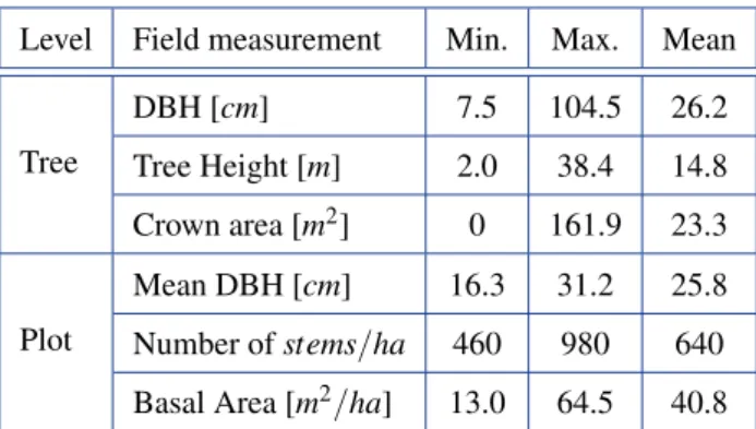
FAO [1] defines an individual tree as “a woody perennial with a single main stem, or in the case of coppice with several stems, having a more or less definite crown". Although this definition denotes a compositional and structural description, it does not consider quantitative aspects such as radiometric or geometric features. It reveals conceptual vagueness relative to an objective physical property [28], which is not precise for inventory purposes. This leads us to quantify a set of measurements in order to characterize trees, for instance: tree height, stem length, crown length, diameter at breast height, and crown area [29]. From these measurements, it is possible to estimate more complex tree variables such as above-ground biomass of trees [30,31].

(16)

1.1. Forest

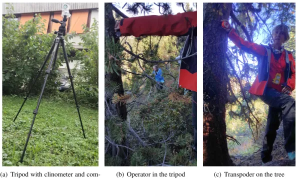
(a) Plot 3b (b) Plot 4

Figure 1.4: Forest inventory carried by the staff of INRAE (Institut national de recherche pour l’agriculture, l’alimentation et l’environnement) in the site of Chamrousse in summer 2018.

1.1.3 The scope of forest inventories

The purpose of ensuring sustainable forestry management requires to assess the current forest con-ditions, extent and quantity through inventory plots as we observe in Figure1.4. Forest inventory is used to understand the development of forest trees by estimating means and totals for measures of forest characteristics over a defined area [32–34]. The possibility of monitoring individual tree architecture has great potential [35,36]. For instance, information on tree crown 3D architecture will help researchers understand the mechanisms underlying competition and growth [37,38]. Be-sides, the ability to monitor forest growth and mortality at the tree level will help forest managers to understand and then prevent the effects of climate change on stand dynamics.

Our understanding of the effect of competition on tree growth is mostly based on field diameter measurements [38]. Tree growth models are important tools to predict the development of each tree within a forest [39]. This type of models consists of diameter and height increment functions to forecast the growth and the mortality probability for each tree in a predefined time interval [40]. The tree growth is not independent of its neighbor’s growth. There is a competition for performing photosynthesis and for accessing to the light and mineral nutrients. The link between the stand level and the individual tree level can be given by important competition variables described by the crown ratio and the open grown trees overlapping [41]. An accurate tree characterization provides relevant inputs to support these deterministic models. Such knowledge will help forest managers adapt their practices toward species mixture, which is often proposed as a way to improve forest resilience in the context of climate change [42], or different diameter structures [43].

In a field survey, forestry technicians collect data on the ground by applying sampling proce-dures [44]. Conventionally, systematic sampling is more efficient for representing land distribu-tion. The sampling units may be stands, plots, strips or points; by having circular, rectangular or square plots [33,44]. The size and the number of plots are defined according to the expected num-ber of measurements, the parameters of interest and the statistical precision. However, field-based inventories are time-consuming and labor-intensive to be collected, providing rough estimates of stand attributes with typical limitations in the sampling because of terrain or vegetation fac-tors [45]. Due to the large extensions of forest, measurements from the ground represent a real challenge for human intervention, involve important costs in employing measurement crews and provide a limited number of individual stands [30]. Remote sensing technologies are applied either for full-cover (entire area of interest) or sampling approaches (sample area). The advancements of remote sensing offer a faster and less expensive collection and analysis of georeferenced data [46] from ground-based, atmospheric and Earth-orbiting platforms [47] for large areas.

(17)

(a) The RGB color model involves the combina-tion of red, blue and green bands from the visible spectrum.

(b) Electromagnetic spectrum of different ranges of energy de-scribed by the wavelength values [51].

Figure 1.5: (a) Illustration of the visual color perception model incorporated in the RGB cam-eras. (b) Description of the electromagnetic spectrum according to different ranges of energy characterized by the wavelength.

1.2 Principles of remote sensing

The remote sensing term was first conceived by Evelyn Pruitt of the US Office of Naval Re-search in the 1950s [48]. It is defined as the science of information acquisition concerning the Earth’s surface without having contact with it [49,50]. This technology makes use of the properties of electromagnetic wave emitted, reflected or diffracted by the sensed objects [51]; for the purpose of processing, analyzing and employing this information [52]. The human visual perception is able to retrieve information in the visible light from the electromagnetic spectrum (see in Figure1.5) in the range between 400 - 700 nm. The color information that we perceive, can be represented by combining the data that comes from three channels or bands: blue (B, 440 - 510 nm [53]), green (G, 540 - 560 nm [54]) and red (R, 630 - 685 nm [53]). In this way, RGB camera in Figure1.5(a) combines the RGB bands for approaching our visual perception. The advantage of the instrumen-tation in remote sensing is these devices are designed to detect all other forms of electromagnetic energy beyond the visible light. For instance, it is possible to cover the infrared information in the range of 700 - 1000 nm of the electromagnetic spectrum in Figure1.5(b).

Remote sensing instruments can be divided into two groups: passive and active sensors [50,

51]. Passive sensors use natural energy from the sun as a source of illumination. In this group, there are radiometers for measuring the intensity of electromagnetic radiation in select bands; and spectrometers, which are designed to detect, measure, and analyze the spectral content of reflected electromagnetic radiation [55,56]. In a different manner, active sensors are character-ized by providing their own source of illumination, and by measuring the energy that is reflected back. This group includes different types of radio detection and ranging (radar) sensors, altime-ters, and scatterometers. The majority of active sensors operate in the microwave band of the electromagnetic spectrum, which gives them the ability to penetrate the atmosphere under most conditions [55,56]. In forest monitoring, the main goal is to extract forest variables by taking advantage of the instruments carried aloft in spaceborne [57,58] or airborne acquisitions such as Goddard’s LiDAR, Hyperspectral and Thermal (G-LiHT), which provides an analytical framework for plant species composition, plant functional types, biodiversity, biomass and carbon stocks, and plant growth [59]. Following the remote sensing instrumentation, we review the principles of two types of technologies: hyperspectral imaging and LiDAR.

(18)

1.2. Principles of remote sensing

(a) A cross-track line recorded by a push-broom imaging sensor on the aircraft [64].

(b) Light dispersion onto a two-dimensional array of detectors in an imaging spectrometer [64].

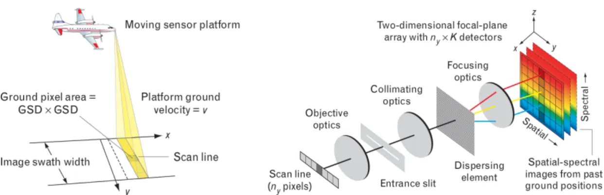
Figure 1.6: Mechanism for hyperspectral data acquisition on the aircraft. (a) The geometry of the push-broom data-collection. (b) An imaging spectrometer disperses light onto a two-dimensional array of detectors.

1.2.1 Hyperspectral imaging

Hyperspectral imaging was first mentioned in the scientific community for discussing the results of imaging spectrometry in 1985 [60]. This passive remote sensing technology deals with the information extracted from objects or scenes lying on the Earth surface, by measuring the radiance acquired by airborne or spaceborne sensors [61] in hundreds of contiguous, registered, spectral bands [60]. A hyperspectral image is formed by two spatial dimensions and one spectral dimension [62]. Taking advantage of this information, we are able to monitor phenomena that could not be detected with a broadband imaging system [47]. We focus on those bands covering the visible, near-infrared, and shortwave infrared spectral bands in the range from 300 to 2500 nm [63].

Push-broom imaging sensor is a common format for hyperspectral data acquisition on the aircraft, as it is observed in Figure1.6. A cross-track line of spatial pixels is decomposed into K spectral bands. The area coverage rate is the swath width times the platform ground velocity v. The area of a pixel on the ground is the square of the ground sample distance (GSD), as we see in Figure1.6(a). The spectral decomposition is carried out by using any of several mechanisms, such as a diffraction grating or a wedge filter [64]. An imaging spectrometer disperses light onto a two-dimensional array of detectors. The spatial dimension contains nyelements in the cross-track

axis, and the spectral dimension is formed by K elements; by obtaining a total of N = K × ny

detectors, as it is represented in Figure1.6(b).

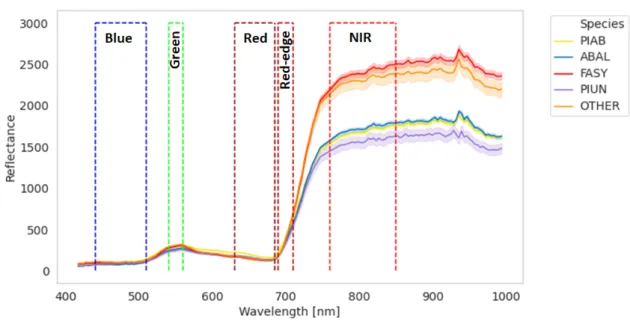
For forestry purposes, hyperspectral data provides absorption features of the vegetation, which are associated to the biochemical attributes to estimate foliage components. In Figure1.7, we show the mean spectral signatures of four main species of the Chamrousse site in the Northern Alpes, France. In addition to the RGB bands, another two important regions are identified from research studies: red-edge band in 690 - 710 nm [54] and near-infrared (NIR) in the range of 760 - 850 nm [53]. This information is relevant for forest applications [49,65] for detecting plant stress [66], measuring chlorophyll content [54,67–71], identifying small differences in percent of green vegetation cover [69,72–76], discriminating land-cover types [77–80], sensing subtle vari-ations in leaf pigment concentrvari-ations [54,68,69,73,81–83], improving the detection of changes in sparse vegetation, assessing absolute water content in leaves [73,84], among others. In this context, spectral information collected from forests is sensitive to the complexity of the canopy structure, because of the disparate configuration of trees [85]. Foliage and branches may be in-terfered with background reflectance when interacting with incoming radiation, which introduces uncertainty in the measurements [86,87]. Depending on the application, it is important to ensure

(19)

Figure 1.7: Mean spectral signatures of four main species located in the Chamrousse site, in the Northern Alpes, France: Abies alba (ABAL), Fagus sylvatica (FASY), Picea abies (PIAB), Pinus uncinata (PIUN) and “other" species. The spectral bands of blue, green, red, red-edge and NIR are higlighted in their respective ranges.

the most effective and efficient use of hyperspectral information. Data processing methods are con-cerned on extracting feature descriptors by identifying and removing the redundant bands [88]. In this thesis, the hyperspectral limitations are addressed by integrating complementary and indepen-dent information for exploring the vertical dimension of the canopy through the LiDAR data.

1.2.2 LiDAR

The laser technology was firstly approached by Charles Townes and Arthur Schawlow in Bell Labs in 1958 [89]. Among the innovative results of this emerging technology, a new generation of sensors and instruments are available nowadays. For instance, LiDAR technology has con-tributed in different applications such as: topographic mapping, flood risk assessments, watershed analysis, forestry modeling and analysis, habitat ecology, landslide investigation, 3D building modelling, road extraction and snow depth measurement [89–91]. LiDAR is an acronym for light detection and ranging [47]. The airborne LiDAR provides the explicit 3D coordinates (x, y, z) of a point cloud, return intensity, return number, number of returns, point classification, among other attributes [92]. In comparison with other remote sensing modalities, the depth measurement provided by airborne laser scanning (ALS) is clearly unique [47]. The term airborne laser is fre-quently associated to those systems that acquire LiDAR data from aircraft. The basis of all ALS systems is emission of a short-duration pulse of laser light and measurement of the elapsed time between emission and detection of the reflected light back at the sensor [62].

A common LiDAR system in Figure1.8consists of a laser scanner coupled with Global Posi-tioning System and Inertial Navigation System (GPS/INS) navigation components, as a means of geo-referencing the position and orientation of the platform’s movement [89,93]. A wide swath is produced by the laser scanner mounted on the platform over which the distances to the mapped surface are measured [89]. The distances from the sensor to the mapped surface are computed by the time-of-flight between the laser pulse transmission and detection [90,94]. Figure1.8(a)shows the data acquisition for three scenarios. In the first scenario, the laser pulse creates three distinct echoes after hitting the canopy. A remaining fraction of the laser pulse hits the ground providing rise to a last echo. In the second scenario, the laser beam is reflected from a sloping surface,

(20)

yield-1.3. Motivation

(a) (1) Laser pulse creates three distinct echoes from canopy. (2) The laser beam is reflected from a sloping surface. (3) The pulse is reflected from a flat surface [94].

(b) Cross section showing LiDAR point cloud data (above) and the corresponding landscape profile (below).

Figure 1.8: (a) LiDAR data acquisition for three scenarios. (b) LiDAR point cloud profile visual-ization.

ing an extended echo pulse width. In the third scenario, the pulse is reflected from a flat surface, resulting in a single echo with a similar amplitude as of the outgoing laser pulse. Then all types of information are used in the post-processing in order to calculate the coordinates of the 3D point cloud as we observe in Figure1.8(b).

LiDAR data is a useful tool to describe the 3D topographic profile of the Earth’s surface, veg-etation cover, and man-made objects [89], hence, the 3D structure of forest. In fact, LiDAR tech-nology has provided outstanding results for estimating measurements of tree height [45,95–98], canopy size [45,96–98], and modeling [99], forest inventory [45,95,97], forest fuel model-ing [100,101], forest structure characterization [102], etc. Describing the forest at the tree level rather than with statistical point cloud metrics makes it easier to propose relevant conservation ac-tions to forest managers. In the last years, decision makers benefited from available forest inven-tory approaches based on ALS [103]. The density improvement of ALS data collections makes the inventory more intuitive by applying individual tree crown (ITC) segmentation techniques [104]. However, the spectral and spatial information from LiDAR data is limited to describe general groups of species, for instance, conifers and broadleaves [85]. Then, the integration of LiDAR data with hyperspectral images can be more efficient for describing species composition.

1.3 Motivation

Forests have played a key role for the planet evolution, influencing all life forms and becom-ing primary source for supplybecom-ing human needs. Therefore, it makes sense that these environments were tremendously affected over time. For instance, the forest cover in France decreased dur-ing the middle age as consequence of the intensity of land use, such as agriculture and human settlements [105]. The pressure on forest came to a maximum at the beginning of the industrial revolution before coal and oil were used as energy sources. Mining, glass making, brick making, and the metal working industries were dependent on wood or on charcoal made from wood [16].

(21)

Forest area has been increasing from now on, especially after the interruption of traditional farming practices [106]. The distance from core areas of economic and urban development pro-duced agricultural land abandonment, mainly in remote areas, such as mountains; where agricul-ture is not economically sustainable [107,108]. This goes hand in hand with the advancement of efficient policies oriented to lower fossil emissions by using forests, either as substitution for non-renewable sources or for carbon storage [109,110].

Mountain forests provide environmental ecosystem services (EES) to communities: supplying of recreational landscapes [111], protection against natural hazards [112,113], supporting bio-diversity conservation [114], among others. Forest stands are also characterized by the species mixture and complex distribution of canopy structure [102]. In order to manage forests in such a way to balance and maintain those EES through space and time [112,115], a good knowledge of the resource (location) is required.

Mountain forests stands are very heterogeneous and timber harvesting is really challenging in these areas due to the slope and terrain roughness [116]. As a consequence, timber harvesting is economically possible but for trees of higher value. This is why we are interested to map each tree and estimate its characteristics, including quality, which is related to its shape and growth conditions. Forest trees are well described by biophysical and biochemical parameters [85,86]. For instance, the tree height, the crown length, the crown area, the crown radius, the diameter at breast height are biophysical descriptors of individual trees. The species composition at leaf level are characterized by the biochemistry of the foliage components, which can be described by the pigment concentration, the water content or the dry matter content [85].

Field inventories are not able to provide a wall to wall cover of detailed tree-level information on a large scale due to topography conditions in mountainous regions, which usually incur much higher expenses. On the other hand, remote sensing tools seem to be a promising technology characterized by the time efficient and the affordable costs for studying forests areas. For in-stance, LiDAR data provide detailed information from the vertical distribution and location of the trees [85,86]. This makes it suitable for single tree detection and crown delineation [45,96–98], from which is possible to derive biophysical parameters. However, single-wavelength measure-ments by LiDAR systems do not provide enough information for estimating biochemical prop-erties, which limits the potential for mapping forest tree species [85,86]. Hyperspectral data are associated to absorption features in the canopy reflectance spectrum, which generate abundant in-formation for the characterization of tree species at pixel level [85]. However, the complexity of canopy structure and the illumination conditions influence the spectral measurements, beyond the limitations in exploring the vertical dimension and the spatial resolution.

The development of hyperspectral and LiDAR sensors has captured the attention of several scientific contributions that seek the fusion of this information with applications to sustainable management of forests for trees characterization. Hyperspectral and LiDAR systems provide in-dependent and complementary data that are relevant for the assessment of biophysical and bio-chemical attributes of forested areas [85]. To go further, the following questions are addressed in this work. First, if the method to be used for data fusion is according to the variables to pre-dict, how data processing methods are applied in each level of data fusion for forest monitoring? Within this purpose, different taxonomies have been proposed to group methods toward data fu-sion [87,117,118] for forest monitoring [119,120].

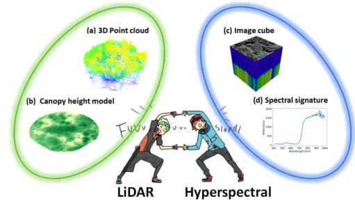
The performance of these methods is associated to the spatial and spectral resolution of the remote sensing data. LiDAR data acquisitions of high spatial resolution provide the conditions to delineate individual trees with high accuracy. Then, if we consider the shape and the size of individual trees, how a crown shape model can improve the segmentation of individual tree crowns? Finally, if LiDAR and hyperspectral data can be used to estimate biophysical and bio-chemical parameters, which combination of feature sets contribute to characterize the forest tree species composition? The purpose of this thesis is to answer these three questions by reviewing and exploring unsupervised and supervised machine learning techniques (Figure1.9).

(22)

1.3. Motivation

Figure 1.9: Data fusion of LiDAR and hyperspectral data: (a) 3D point cloud from LiDAR data. (b) 2D LiDAR representation in the canopy height model. (c) Image cube representation of all the bands in the hyperspectral image. (d) Spectral signature of a pixel in the hyperspectral image.

To answer the first question, a literature review of data fusion of LiDAR and hyperspectral data for forest monitoring, has been organized in different methods and levels. Most of the authors con-verge at three levels of data representation [87,117–120]: low level or observation level, medium level or feature level, and high level or decision level. The first level consists of the integration of reflectance information and the coordinates of LiDAR points for alignment [117]. Although, the output of this level of fusion by itself does not provide explicit information for forest application, the corrected data reduces geometric and radiometric distortions. The second level is about the extraction of feature descriptors to form a new set of data representation [117]. At this level of fusion, a new feature set derived from the LiDAR and hyperspectral data, can provide more con-sistent and discriminatory information to establish relationships with forest tree composition. The majority of fusion schemes reaches the decision level, in which each modality is processed inde-pendently to develop rule-based models [117–119]. Several studies use the supervised methods to integrate features from different remote sensing modalities for species mapping [69,121–135], the estimation of functional, physiological [54,73,136–149] and structural attributes [150–158], above-ground biomass and carbon density [74,159–162], and land cover maps [77–80].

Airborne data vendors provide remote sensing acquisitions processed at low level fusion by applying geometric and radiometric corrections [77], and by exploiting the high spatial resolution of LiDAR data. In fact, if LiDAR technology can describe in detail the canopy vertical distribu-tion [85], it seems consistent to use these data to answer the second question, how a crown shape model can improve the segmentation of individual tree crowns? In several studies, the individual tree crown (ITC) delineation can be posed as a 3D segmentation approach using a LiDAR point cloud [163]. Studies for automatic segmentation of trees [96,97] extract tree crown shape informa-tion by using allometric equainforma-tions in order to estimate the parameters of the algorithms. We pro-pose a new framework for ITC delineation by introducing a crown shape model [164]. A proper ITC delineation provides accurate estimation of the crown architecture given by the tree height, the crown area, the crown radius and the crown height [45,96–98]. In addition to that, the information obtained from the ITC delineation can serve as an input for later stages of processing LiDAR and hyperspectral data at decision level fusion, such as tree species classification [159,165].

To answer the third question, which combination of feature sets contribute to characterize the forest tree species composition?, we focus on the data fusion at medium and high level. At medium level, we proceed to extract feature descriptors from each modality [69,130,132,135]. Features

(23)

can be computed at point, pixel and object (tree) level. Dechesne et al. [165] suggest to rasterize the point features from LiDAR data in order to be aligned with the hyperspectral grid. From the hyperspectral data, we extract vegetation indices that has been demonstrated in other studies to characterize forest tree species [69,74,76]. We propose an approach for selecting features that produce a better forest tree species classification. The present dissertation contributes to the understanding of forest characteristics by exploiting hyperspectral images and LiDAR data, by combining these two modalities to derive tree species composition within a heterogeneous canopy of a mixed forest.

1.4 Objectives

In this thesis, we present the integration of remotely sensed data for the analysis of forest areas. In particular, we focus our attention on hyperspectral and LiDAR data that are of primary impor-tance in the study of forest areas. Our attention is also devoted to the use of unsupervised and supervised machine learning techniques for the use of the information contained in such data ac-quired over forest areas. To summarize, the thesis objectives answer the three scientific challenges described in Section1.3, more specifically, we address the following questions:

• Q1. How data processing methods are applied in each level of data fusion for forest moni-toring?

The last review of data fusion for forest monitoring was carried in 2014 [87]. Since then, new contributions have emerged to tackle this problem [166,167]. We propose a literature review on the integration of hyperspectral imaging and LiDAR data by grouping data pro-cessing methods in general process at each level of data fusion, by illustrating the potential relationships found in these studies. Although different authors propose a variety of tax-onomies for data fusion, we classified our reviewed methods according to three levels: low level or observation level, medium level or feature level, and high level or decision level. This review examines the relationship between the three levels of fusion and the methods used in each considered approach. A set of 50 contributions oriented to forest monitoring applications that combines hyperspectral images and LiDAR data at different levels of fu-sion are reviewed. This work was published in the book series "Data Handling in Science and Technology" in January 2020 and the work is presented in Chapter2:

TUSA, E., LAYBROS, A., MONNET, J. M., DALLAMURA, M., BARRÉ, J. B., VINCENT, G., DALPONTE, M., FÉRET, J. B. CHANUSSOT, J. (2020). FUSION OF HYPERSPECTRAL IMAGING AND LIDAR FOR FOREST MONITORING. IN Data Handling in Science and Technology(VOL. 32,PP. 281-303). ELSEVIER.

• Q2. How a crown shape model can improve the segmentation of individual tree crowns? Ferraz et al. [96,97] proposed the adaptive 3D mean shift (AMS3D) for ITC delineation. This approach is based on adaptive kernel size that is suitable for tropical forests, but it could lead to an undersegmentation effect by merging adjacent coniferous tree crowns. We present an AMS3D approach based on the adaptation of the kernel profile size through an ellipsoid crown shape model, which fits the coniferous tree crowns that are present in tem-perate forests. The algorithm parameters are estimated based on allometry equations derived from 22 forest plots in two study sites described in Chapter3. The ellipsoid crown shape model with a superellipsoid (SE) kernel profile of n = 1.5 presents the highest recall and the best Jaccard index, especially for conifers. This work was published in the journal "IEEE Geoscience and Remote Sensing Letters" in August 2020 and it is presented in Chapter4:

(24)

1.5. Thesis structure

TUSA, E., MONNET, J. M., BARRÉ, J. B., DALLAMURA, M., DALPONTE, M., CHANUS -SOT, J. (2020). INDIVIDUAL TREE SEGMENTATION BASED ON MEAN SHIFT AND CROWNSHAPEMODEL FORTEMPERATEFOREST. IEEE Geoscience and Remote Sensing Letters.

• Q3. Which combination of feature sets contribute to characterize the forest tree species composition?

We aim to investigate the integration of feature descriptors from HI and LiDAR by using the intra-set and inter-set feature importance by using random forest (RF) score and 5-fold cross validation. We consider the following feature sets: 160 hyperspectral bands (HI), 61 vege-tation indices detailed in chapter2, the principal components (PC) obtained by using robust PCA (rPCA) [127] from HI, 72 LiDAR features explained in [165], and their PC by using rPCA. Previously, the dataset is created from the field inventory information by projecting the tree crowns, by selecting the non-overlapping pixels and by removing pixels associated to non-vegetation, low objects and shadow. RF is aplied for the feature classification [76]. The overall accuracy of tree species classification at pixel-level was 78.1%. Our approach showed that 78.3% of trees were correctly assigned overall, by having conifers such as Nor-way Spruce (Picea abies) and mountain pine (Pinus uncinata) with producer’s accuracies above 90%. This approach was presented in the conference "XXIV International Society for Photogrammetry and Remote Sensing (ISPRS) Congress" in August 2020 and the work is detailed in Chapter5:

TUSA, E., MONNET, J. M., BARRÉ, ,J.B., M, D. M., CHANUSSOT, J. (2020). FUSION OF LIDAR ANDHYPERSPECTRAL DATAFOR SEMANTIC SEGMENTATION OF FOREST TREE SPECIES. Int. Arch. Photogramm. Remote Sens. Spatial Inf. Sci., XLIII-B3-2020, 487–494, 2020. DOI:HTTP://DX.DOI.ORG/10.5194/ISPRS-ARCHIVES -XLIII-B3-2020-487-2020

1.5 Thesis structure

This work is divided in 6 chapters:

• Chapter 2 presents and discusses the existing methods for data fusion by defining three levels: low- or observation-level, medium- or feature-level and high- or decision level. Dif-ferent forest monitoring applications are reviewed according to these levels of fusion. • Chapter3describes the datasets used for the algorithm assessment: the study areas

compo-sition, the field data procedures and instruments, and the specifications of the remote sensing instruments.

• Chapter4presents the ITC delineation method based on 3-D Adaptive Mean Shift (AMS3D) and the ellipsoid crown shape model by adapting the kernel and the influence for detecting conifers and broadleaves.

• Chapter5explains the tree species classification approach for the integration of LiDAR and hyperspectral information, by selecting feature descriptors and by transforming feature sets into a new feature space.

• Chapter6presents conclusions and perspectives for this thesis.

(25)

(26)

2

Data Fusion

Hyperspectral data contains meaningful reflectance attributes of plants or spectral traits, while LiDAR data offers alternatives for an-alyzing structural properties of canopy. The fusion of these two data sources can improve forest characterization. The method to use for the data fusion should be chosen according to the variables to pre-dict. This chapter presents a literature review on the integration of hyperspectral imaging and LiDAR data by considering applications related to forest monitoring. Although different authors propose a variety of taxonomies for data fusion, we classified our reviewed methods according to three levels of fusion: low level or observa-tion level, medium level or feature level, and high level or decision level. This review examines the relationship between the three levels of fusion and the methods used in each considered approach.

Sommaire 2.1 Principles of fusion . . . 16 2.2 Low-level . . . 17 2.2.1 Geometric correction . . . 17 2.2.2 Radiometric correction . . . 19 2.3 Medium-level. . . 19 2.3.1 Feature extraction. . . 19 2.3.2 Feature stacking . . . 26 2.3.3 Feature selection . . . 26 2.3.4 Feature fusion. . . 27 2.4 High-level. . . 27 2.4.1 Classification . . . 27 2.4.2 Segmentation . . . 28 2.4.3 Data association . . . 29 2.4.4 Prediction-estimation . . . 29 2.5 Applications . . . 29 15

(27)

Chapter 2. Data Fusion

2.1 Principles of fusion

As we mentioned in chapter 1, LiDAR data provide detailed geometric information, which makes it suitable for single tree detection and crown delineation [45,96–98]. However, single-wavelength measurements by LiDAR systems is not enough for estimating biochemical properties, which is meaningful for mapping forest tree species [86]. At the same time, hyperspectral data de-scribe a bi-dimensional representation of absorption features in the canopy reflectance spectrum, which allows the characterization of tree species at pixel level. However, the spectral measure-ments are sensitive to the complexity of the canopy structure and the illumination conditions [85]. The purpose of integrating remote sensing modalities is to achieve fused data from informa-tion of different spatial, spectral and temporal resoluinforma-tions [118]. The output of the integration of these complementary and independent data is more refined, more robust and more accurate than individual data sources [117]. In this manner, data fusion improves the quality of information for decision making, by benefiting from the development of hyperspectral and LiDAR sensors. The problem of data fusion has captured the attention of several scientific contributions that seek for applications of main interest for sustainable management of forests: from trees to stand character-ization [119,120,124].

Data fusion [117,118,168] gathers a group of methods and approaches that combines multiple sources of data. Particularly, different categories have been proposed to describe the fusion of hyperspectral images and other remote sensing modalities [117,118], such as LiDAR data for forest monitoring [119,120,124]. Table2.1summarizes the main fusion categories considered in different studies: domain, resolution, nature of images, methods and data processing. Focusing on our interest of data processing, all the authors converges at three level of data representation defined clearly by Dechesne [165] as follows: low level or observation level, medium level or feature level, and high level or decision level. In this chapter, these three categories are going to be studied according to our literature review on data fusion for forest applications.

Table 2.1: Fusion categories (domain, resolution, nature of images, method and processing) de-scribed by levels proposed by five different authors. For data processing, three levels are defined: low level or observation level, medium level or feature level, and high level or decision level.

Categories Authors Chaudhuri et al. [117] Kandare [120] and Torabzadeh et al. [124] Pohl et al. [118,168] Dechesne [119] Domain Spatial Frequency Resolution Pan-sharpening Nature of images Multimodal image

fusion Method Empirical or statistical Physical Hybrid Processing

Pixel or signal Data Subpixel Observation

Pixel

Feature or region Product Feature

(28)

2.2. Low-level

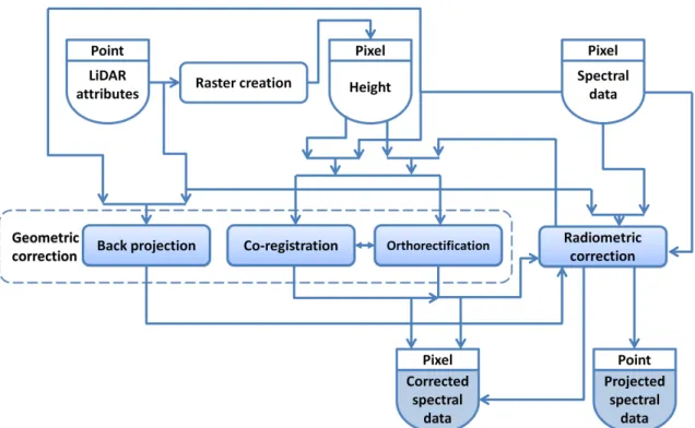
Figure 2.1: Graphical representation of processes for ilustrating fusion methods: a) Unit of data symbolizes the spatial space and the type of information. b) A block expresses the task for pro-cessing data and information. c) Interaction arrow for representing the inputs and outputs of processing blocks. d) Input simultaneity to a processing block

For each level of fusion, diagrams that describe interactions among processes and their in-puts and outin-puts, illustrate the processes involved at each level. Units of data are represented in Figure2.1 a), for clarifying how data evolves through every processing task. Every unit of data describe the type of information: spectral bands, height, feature, and so on; and also, the spatial space in which this information is represented: point level, pixel level, region level and object level. Additionally, a block represents tasks for processing data and information as it is observed in Figure2.1 b), and finally, the arrows in Figure2.1 c) and d) depict the interactions between these units of data and processes.

2.2 Low-level

This level is the most basic and fundamental fusion for understanding and processing the data [117]. It corresponds to the fusion of the reflectance of hyperspectral images and the coor-dinates of LiDAR point cloud [119]. This level of fusion preserves most of the original informa-tion [118]. In Figure2.2, we describe processes for geometric and radiometric correction.

2.2.1 Geometric correction

Geometric correction is concerned with placing spectral information in their proper planimetric (x, y) map location so it can be associated with other spatial information [169]. This task involves different data fusion processes. Some studies correct distortions from the point cloud coordinates by using real world coordinates pixels [154] or by direct georeferencing [130]. Geometric correc-tion algorithms are implemented in several computacorrec-tional packages: Tiff [144], CaliGeo available in ENVI [160], and HyperspecIII software [131,133]. In this review, we are concerned about three types of geometric correction: orthorectification, co-registration and back projection.

Before explaining the geometric correction processes, it is imperative to define the canopy height model (CHM), which is the most common raster representation of LiDAR data for fusion at this level. CHM can be created in different ways. First, the point cloud is classified as ground and vegetation points by using the TerraScan software [159,170]. Then, the digital terrain model (DTM) is derived from the ground points, and the digital surface model (DSM) from all the points. The CHM is simply computed by subtracting the DTM from the DSM. A second approach is based on the creation of a terrain surface, which is not necessarily a DTM; for instance, a TIN surface.

(29)

Figure 2.2: Illustration of fusion at low level or observation level

Then, the point cloud is normalized to compute directly a CHM that can be slightly lower than the one obtained in the first approach. Several studies prefer the use of specific softwares for creat-ing the CHM: Tiff [156,171], TerraScan [128,151,152], FUSION [139,172], eCognition [129], LAStools[78,158]. When CHM contains empty pixels called "pits", the R package lidR [173] implements a pit-free algorithm for LAStools following the method proposed by [174]. Addition-ally, CHM is used to threshold forest from forest gaps and low canopy heights [80,126], or for establishing a framework for extraction of features [122].

The processes of orthorectification and co-registration can be applied separately or integrated as a workflow. Orthorectification is the process of geometrically adjusting the hyperspectral im-age to an orthogonal imim-age (DSM) by transforming coordinates from the imim-age space to the ground space and removing tilt and relief displacement, for creating a planimetrically correct image [169,175]. Usually, remote sensing images are orthorectified and georeferenced before being sent to users. Sometimes these procedures are not accurate enough to identify individual trees. Co-registration methods for remote sensing datasets of wooded landscapes can improve the results [77]. For instance, the AROP package performs automated precise registration and orthorectification [176].

Co-registration is the translation and rotation alignment process in order to obtain a registered hyperspectral image by considering the LiDAR-derived DSM as reference [169]. This task has demonstrated the effectiveness and potentialities for decision-level process such pixel classifica-tion [177]. The process of co-registration of two image modalities requires the use of ground con-trol points (GCP) [121]. Shen et al. [69] apply the nearest-neighbor interpolation by using more than 30 GCP with an accuracy of 0.25 m. Alonzo et al. [123,137] use Delaunay triangulation with 137 GCP. Alternatively, other approaches do not require GCP for the registration process. For instance, the NGF-Curv algorithm proposed by Refs. [77,127,156] is based on the minimization of an objective function that contains similarity and regularization terms. NGF-Curv algorithm is implemented in the image registration software package called FAIR [178]. A second approach that avoids GCP is implemented in the GeFolki package [179], which is based on a local method of optical flow derived from the Lucas-Kanade algorithm, with a multiscale implementation, and

(30)

2.3. Medium-level

a specific filtering including rank filtering. The disadvantage of the registration methods without GCP is these are biased by shading effects, which are present in mountainous forest.

Back projection of LiDAR point cloud onto the image plane allows a better co-alignment than the image orthorectification with the CHM because of altitude distortions associated with the irregular porous surface of forest canopy. Back projection was implemented by Brell et al. [180] on hyperspectral imagery, by improving the geometric alignment between the hyperspectral images and LiDAR data. Alternatively, the process of spectral projection onto the 3D point cloud is implemented by Asner et al. [134], through a sun-canopy ray tracing for sunlit. In this way, LiDAR data with known solar position provided 3D maps of illumination geometry for each canopy.

2.2.2 Radiometric correction

The radiometric correction aims at converting radiance values of hyperspectral images into re-flectance [169]. In the forest monitoring applications, authors do not establish a strict sequence for applying radiometric correction. In some studies, images are atmospherically corrected before co-registration by using the Atmospheric and Topographic Correction software ATCOR-4, which implements the radiative transfer model MODTRAN [54,77,123,130,132,136,137,142,144,148,

154,160]. Another task based on MODTRAN model for minimizing atmospheric effects, it is implemented in the Fast Line-of-Sight Atmospheric Analysis of Spectral Hypercubes, FLAASH algorithm, which is available in the image analysis software ENVI [74,122,128,135,143,181]. Alternatively, the model ACORN is used to improve aerosol correction [78,145–147,149]. Ad-ditionally, there are other algorithms implemented in SpectralView [131,133] or QUAC [73] for these correction purposes.

Another strategy for radiometric correction is implemented through normalization algorithms. For instance, the value of each pixel was normalized with respect to the sum of the original values of the same pixel in all the bands, by resulting in a significant improvement of the final classifi-cation accuracies [159]. This relative radiometric normalization is applied to the single images to obtain a uniform mosaic image [121]. The radiometric correction implemented after back pro-jection involves a fusion strategy, by comparing the LiDAR return intensity and the hyperspectral information at the same wavelength [182]. This procedure requires spectral information beyond the VNIR spectral range.

2.3 Medium-level

Feature descriptors provide complementary information that is combined to form a composite set of features [117]. In this section, our literature review considers four important processes illustrated in Figure2.3: feature extraction, feature stacking, feature selection and feature fusion.

2.3.1 Feature extraction

The main goal of these features is to represent the most relevant information from the original data [183]. From the fusion approaches, we have identified the following groups of feature descriptors: statistical, structural, topographic, vegetation indices, textural and dimension reduction.

• Statistical features have been widely used for forest tree characterization. In Table2.2, a summary of statistical features are associated with their references and the data source: height from 3D point cloud, return intensity, CHM and spectral band. For instance, Dech-esne et al. [165] compute these features by using three cylindrical neighborhoods around

(31)

Figure 2.3: Fusion at medium level or feature level

each LiDAR point. Then, these features are projected on the CHM. In parallel, a set of statistical descriptors is computed at each spectral band by considering the same cylindri-cal radius. In Refs. [69,73], authors compute these statistical features for every crown, which are extracted manually from field measurements [79] or by applying a segmentation algorithm. A review of segmentation approaches is described in the subsection of fusion at decision level.

• Topographic features or terrain features describe landscape level variations, which are related to the topography or soil [126]. A list of these type of features is described in Table2.3. Cao et al. [75] compute these features from heights at the 3D point cloud. In [54,

126], these features are rasterized into a 2D representation.

• Structural features are summarized in Table2.4, which are derived from LiDAR data. In Refs. [73,123,137,155], authors compute these features by using the point cloud associated to each individual crown, which has been previously segmented in the CHM. Torabzadeh et al. [125] carry out these computations by handling return intensity.

• Vegetation indices (VI) derived from hyperspectral data are organized in 5 groups in the next tables: broadband greenness in Table 2.5, narrowband greenness in Table 2.6, light use efficiency in Table2.7, leaf pigments in Table2.8, dry or senescent carbon and canopy water content in Table2.9. VI provide important radiometric characteristics for quantifying biophysical and biochemical indicators [69]. Studies show different strategies for the com-putation of these features. For instance, La et al. [152] obtain the NDVI index directly from the software ENVI. Kandare et al. [73] works at object level for averaging the pixel values inside every segmented crown at each band for deriving 16 VI. Luo et al. [74] focusing

(32)

2.3. Medium-level

Table 2.2: List of statistical feature descriptors with the respective references divided by the data source: height from 3D point cloud, amplitude of the return signal, CHM or spectral band

No. Statistical feature Point cloud Return intensity CHM Spectral band 1 Minimum [69,165] [139] [165] 2 Maximum [69,73–75,155,165] [139] [165] 3 Mean [74,75,155] [165] [165] 4 Median [165] [165] 5 Standard deviation [69,73–75,165] [139] [165] 6 Variance [73]

7 Median absolute deviation from median

[165] [165]

8 Mean absolute deviation from median

[165] [165]

9 Mean absolute deviation from mean [165] [165] 10 Skewness [73,155,165] [139] [165] 11 Kurtosis [73,155,165] [139] [165] 12 Percentiles [69,73,74,125,155,165] [125] 13 Interquartile distance [69] [139] 14 Coefficient of variation [69,73–75,155] 21

(33)

Table 2.3: List of topographic feature descriptors with the respective references divided by the data source: height from 3D point cloud or CHM

No. Topographic feature

Point cloud

CHM No. Topographic fea-ture

Point cloud

CHM

1 Aspect [162] [126] 2 Foliage height diver-sity

[54]

3 Hillshade [75] [126] 4 Profile curvature [75,162]

5 Slope [75,162] [126] 6 Elevation data [126]

7 Tree height [54] [126] 8 Topographic wetness index

[75]

9 Plant area index [54] 10 Compound topo-graphic index

[162]

11 Disection [162] 12 Heat load index [162] 13 Planar curvature [162] 14 Heat load index [162] 15 Site exposure

in-dex

[162] 16 Surface relief ratio [162]

17 Total curvature [162] 18 Vector ruggedness model

[162]

on the group of narrowband greenness because these VI reduces the saturation effect and improve the biomass estimation.

• Textural features are widely used in computer vision because these contain information concerning the structural arrangement of surfaces and their relationship to the surrounding environment [224]. Gray-Level Co-occurrence Matrix (GLCM) was computed by Dalponte et al. [79] over the band of 810nm. Alternatively, Cao et al. [75] implemented the texture analysis after computing Principal Component Analysis (PCA) over the first component. Plowright et al. [139], extract textural information by using the extended morphological profile method through circular structuring elements over the first three principal compo-nents of the hyperspectral data.

• Dimension Reduction is a special form of feature extraction [183]. Most of the feature ex-traction techniques revised previously, are focused on processing one modality at a time. In Refs. [69,130,132,135], authors apply PCA for obtaining the most meaningful information from hyperspectral metrics. In Refs. [75,151,152], PCA is obtained by using the software ENVI.

In Refs. [127,156], robust PCA (rPCA) is used for feature extraction of hyperspectral im-agery. For tree crown segmentation purposes, the first principal component was ignored because it contained illumination information rather than useful features [225]. The second to fifth principal components were extracted and assigned to corresponding LiDAR points by using horizontal geospatial coordinates.

Zhang et al. [129], segregate spectral noise in hyperspectral data by applying Minimum Noise Fraction (MNF) transformation. This is a linear transformation of the original bands that applies two cascaded PCA and maximizes the ratio of signal to noise. This procedure can be performed in the software ENVI. Dian et al. [128] select the first 10 MNF bands

(34)

2.3. Medium-level

Table 2.4: List of structural feature descriptors with the respective references divided by the data source: height from 3D point cloud or return intensity

No. Structural feature Point cloud Return

ntensity

1 Crown height [123,125,137]

2 Crown widths at selected heights [123,137] 3 Ratios of crown heights to widths at selected heights [123,125,137] 4 Direct measures of return intensity through the crown [123,137]

5 Distributions of intensity through the crown [123,137] 6 Crown porosity measured by return penetration into the crown [123,137] 7 Occupied length of the vertical column by vegetation [125]

8 Number of detected canopy layers [125] 9 Relative position of the largest canopy layer [125]

10 Cumulative intensity [125]

11 Point density [125]

12 Scatter [165]

13 Planarity [165]

14 Number of local height maxima [165]

15 Number of non-ground points within neighborhoods [165] 16 Cumulative proportional canopy density [69,73,155]

17 Canopy volume [155]

18 Crown area [73,73]

19 Laser intercept index [74]

20 Percentage of returns > 0.5m [139] 21 Canopy cover (Percentage of first returns > 2.0m) [69,75]

(35)

Table 2.5: Broadband greenness

No. VI Ref. No. VI Ref

1 Normalized Differ-ence Vegetation Index (NDVI)

[69,72–76] 2 Non-Linear Index (NLI)

[184]

3 Renormalized Differ-ence Vegetation Index (RDVI) [158,185] 4 Modified Non-Linear Index (MNLI) [186] 5 Green Normalized Difference Vegetation Index (GNDVI) [69, 73, 76, 80, 187]

6 Green Leaf Index (GLI) [188] 7 Infrared Percentage Vegetation Index (IPVI) [73,76,189] 8 Transformed Differ-ence Vegetation Index (TDVI) [190] 9 Triangular Greenness Index (TGI) [191] 10 Difference Vegetation Index (DVI) [73,76,192]

11 Green Difference Veg-etation Index (GDVI)

[193] 12 Green Red Difference Index (GRDI) [192] 13 Difference Difference Vegetation Index (DDVI) [76,194] 14 Enhanced Vegetation Index 1 (EVI1) [69,73,74,76,128, 195] 15 Enhanced Vegetation Index 2 (EVI2)

[76,196] 16 Leaf Area Index (LAI) [197]

17 Simple Ratio Vegeta-tion Index 1 (SRVI1)

[69,73–76,126,

198]

18 Modified Simple Ratio (MSR)

[199]

19 Green Chlorophyll In-dex (GCI)

[54,67–69] 20 Green Ratio Vegeta-tion Index (GRVI)

[200]

21 Green Red Ratio Veg-etation Index (GRRVI)

[76,201] 22 Blue Ratio Vegetation Index (BRVI)

[76,201]

23 Red Ratio Vegetation Index (RRVI)

[76,201] 24 Sum Green Index (SGI)

[69,202]

25 Soil Adjusted Vegeta-tion Index (SAVI)

[69,74,75,203] 26 Optimized Soil Ad-justed Vegetation In-dex (OSAVI)

[74,204]

27 Modified Soil Ad-justed Vegetation Index 2 (MSAVI2)

[74,75,158,205] 28 Green Soil Adjusted Vegetation Index (GSAVI)

[193]

29 Green Optimized Soil Adjusted Vegetation Index (GOSAVI)

[193] 30 Green Atmospheri-cally Resistant Index (GARI)

[76,206]

31 Visible Atmospheri-cally Resistant Index (VARI)

[76,207] 32 Wide Dynamic Range Vegetation Index (WDRVI)

(36)

2.3. Medium-level

Table 2.6: Narrowband greenness

33 Modified Normalized Difference Vegetation Index (MNDVI)

[74,210] 34 Red Edge Normalized Difference Vegetation Index (RENDVI)

[76,80,126,211,

212]

35 Modified Red Edge Normalized Differ-ence Vegetation Index (MRENDVI)

[69,76,212] 36 Simple Ratio Vegeta-tion Index 2 (SRVI2)

[74,210]

37 Modified Red Edge Simple Ra-tio (MRESR)

[73,76,212,213] 38 Red Edge Chlorophyll Index (RECI)

[68,69]

39 Vogelmann Red Edge Index 1 (VREI1)

[73,214] 40 Vogelmann Red Edge Index 2 (VREI2)

[214]

41 Red Edge Inflection Point (REIP) [74,126,215] 42 Atmospherically Re-sistant Vegetation Index (ARVI) [73,74,76,216] 43 Modified Chlorophyll Absorption Ratio In-dex 1 (MCARI1)

[70] 44 Modified Chlorophyll Absorption Ratio In-dex 2 (MCARI2) [71] 45 Transformed Chloro-phyll Absorption Reflectance Index (TCARI) [69,71] 46 Triangular Vegetation Index (TVI) [217] 47 Modified Triangular Vegetation Index 1 (MTVI1) [71] 48 Modified Triangular Vegetation Index 2 (MTVI2) [71,158]

Table 2.7: Light use efficiency

49 Photochemical Re-flectance Index (PRI)

[69,76,126,218,

219]

50 Structure Insensitive Pigment Index (SIPI)

[69,73,220]

51 Red Green Ratio Index (RGRI)

[69,221] 52 Photochemical Re-flectance Ratio (PRR)

[69,222]