Learning Multiple Conflicting Tasks with Artificial Evolution

RESEARCH OUTPUTS / RÉSULTATS DE RECHERCHE

Author(s) - Auteur(s) :

Publication date - Date de publication :

Permanent link - Permalien :

Rights / License - Licence de droit d’auteur :

Bibliothèque Universitaire Moretus Plantin

Institutional Repository - Research Portal

Dépôt Institutionnel - Portail de la Recherche

researchportal.unamur.be

University of Namur

Learning Multiple Conflicting Tasks with Artificial Evolution

Nicolay, Delphine; Andrea, Roli; Carletti, Timoteo

Published in:

Advances in Artificial Life and Evolutionary Computation

DOI:

10.1007/978-3-319-12745-3_11 Publication date:

2014

Document Version

Early version, also known as pre-print

Link to publication

Citation for pulished version (HARVARD):

Nicolay, D, Andrea, R & Carletti, T 2014, Learning Multiple Conflicting Tasks with Artificial Evolution. in C Pizzuti & G Spezzano (eds), Advances in Artificial Life and Evolutionary Computation: 9th Italian Workshop, WIVACE

2014, Vietri sul Mare, Italy, May 14-15, Revised Selected Papers. vol. 445, Communications in Computer and

Information Science, vol. 445, Springer, pp. 127-139, 9th Italian Workshop on Artificial Life and Evolutionary Computation, WIVACE 2014, Vietri sul Mare, Italy, 14/05/14. https://doi.org/10.1007/978-3-319-12745-3_11

General rights

Copyright and moral rights for the publications made accessible in the public portal are retained by the authors and/or other copyright owners and it is a condition of accessing publications that users recognise and abide by the legal requirements associated with these rights. • Users may download and print one copy of any publication from the public portal for the purpose of private study or research. • You may not further distribute the material or use it for any profit-making activity or commercial gain

• You may freely distribute the URL identifying the publication in the public portal ?

Take down policy

If you believe that this document breaches copyright please contact us providing details, and we will remove access to the work immediately and investigate your claim.

Learning multiple conflicting tasks with artificial

evolution

D. Nicolay1_{, A. Roli}2_{, and T. Carletti}1

1

Department of Mathematics and naXys, University of Namur, Belgium

2

Department of Computer Science and Engineering (DISI), University of Bologna, Campus of Cesena, Italy

Abstract. The paper explores the issue of learning multiple competing tasks in the domain of artificial evolution. In particular, a robot is trained so as to be able to perform two different tasks at the same time, namely a gradient following and rough terrain avoidance behaviours. It is shown that, if the controller is trained to learn two tasks of different difficulty, then the robot performance is higher if the most difficult task is learnt first, before the combined learning of both tasks. An explanation to this superiority is also discussed, in comparison with previous results.

1

Introduction

Since its first appearance in the late 60’s, artificial evolution (AE) has been suc-cessfully applied to solve a plethora of problems arising in fields such as circuit design, control systems, data mining, optimisation and robotics. The application of AE to robotics is commonly named evolutionary robotics (ER) and it is mainly concerned with the artificial evolution of robots neural controllers [12]. ER has contributed with notable results to the domain of artificial cognition and it also provides a viable way for designing robotic systems, such as robot swarms. Nev-ertheless, in spite of promising initial results, ER has not completely expressed its potential, especially in the design of complex robotic controllers. In fact, ER is still applied with large contributions of the experience and the intuition of the designer. To close the gap between current ER achievements and its potential applications, both theoretical and methodological advancements are required. A case in point is the issue of training a robot controller such that the robot is able to accomplish more than one task at the same time. The practice in robotic learning already possesses some good practice and specific methodologies, such as robot shaping [5], which is primarily applied to incremental training of robots. However, general results in this context are still lacking.

A prominent study is that by Calabretta et al. [3], in which the question as to whether a non-modular neural network can be trained so as to achieve the same performance as a modular one in accomplishing multiple tasks is addressed. The neural network is trained to perform two simultaneous classification tasks on the same input, one task being harder than the other. The conclusion of the

results of these experiments is particularly interesting: the best performance is attained by training first on the harder tasks and successively also on the second. This learning sequence is the one enabling the search process to minimise the so-called neural interference, which appears every time neural weights involved in the computation of both tasks are varied considerably, leading to a detriment of the overall network performance. If the harder task is learnt first, then neural interference is reduced as much as possible, because the magnitude of weight variation is kept at minimal levels. The work by Calabretta and co-authors is particularly meaningful because it sheds light to the mechanisms underpinning the learning sequence that leads to the best performance—which is comparable to the one attained by a modular neural network, trained independently on the two tasks.

In this work, we address the question as to which is the best task learning sequence for training a robot. The case under study is more general than that in [3], as it consists of two conflicting robotic tasks—which are computationally more complex than classification tasks—and both network structure and weights can undergo changes during the training phase, which is based on a genetic al-gorithm (GA). We will show that the best results can be attained by training the robot on the harder task first and then on both tasks, confirming the results in [3]. Nevertheless, since our controllers and the training process are different than those in the study by Calabretta et al., the explanation based on neural interference is no longer valid and a different mechanism should be found. We conjecture that in the case of GA, the interference between the two tasks induces a rugged fitness landscape: learning first on the harder task means to keep the landscape as smooth as possible, thus enabling the search mechanism of GA to attain a higher performance than in the other learning cases.

In Section 2, we illustrate the scenario and two tasks the robot has to perform. In Section 3, we detail the experiments we made and we describe the results of the three possible training settings for the robot. Section 4 presents a discussion on the results and Section 5 concludes the contribution with an outline of future work.

2

Model and tasks description

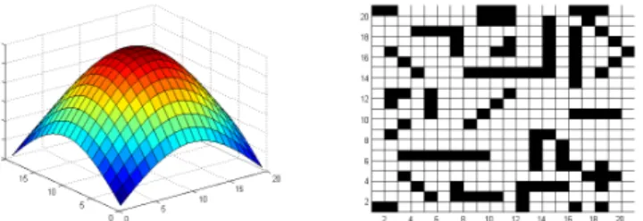
The abstract application that we focus on follows ideas presented by Beau-mont [1]. Virtual robots, controlled by neural networks, are trained to learn two different tasks in a virtual arena. This arena is a discretised grid of varying sizes, hereby for a sake of simplicity we fixed it to 20 × 20, with a torus topology, i.e. periodic boundary conditions on both directions, on which robots are al-lowed to move into any neighbouring square at each displacement, that is the 8–cells Moore neighbourhood. Assuming the arena is not flat and it possesses one global maximum, the first task we proposed involves reaching this global maximum, represented using a colour code in the left panel of Fig. 1; the second task consists in moving as long as possible in the arena by avoiding

“danger-ous”zones, i.e. zones where robots loose energy, represented by black boxes in the right panel of Fig. 1.

Fig. 1. Arenas where robots are trained. Left panel: arena for task T1, the peak level

is represented as a color code: red high level, blue lower levels. Right panel: arena for task T2, black boxes denote the “dangerous”zones to be avoided as much as possible.

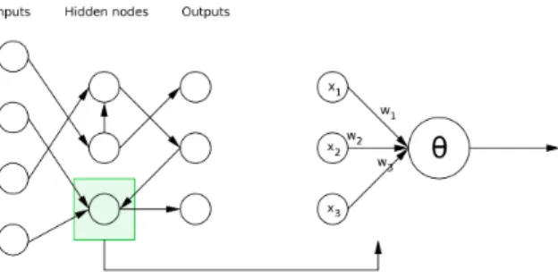
The model of neural networks [13, 14] that we use is schematically shown in Fig. 2. The topology is completely unconstrained, except for the self–loops that are prohibited. Each neuron can have two internal states: activated (equal to 1) or inhibited (equal to 0). The weight of each link is 1, if the link is excitatory, or −1 if it is of inhibitory nature. Given the present state for each neuron, (xt

i), the

updated state of each neuron is given by the perceptron rule:

∀j ∈ {1, . . . , N } : xt+1_j =      1 if kin j P i=1 wt jixti≥ θkjin 0 otherwise where kin

j is the number of incoming links in the j–th neuron under scrutiny, θ

the threshold of the neuron, a parameter lying in the interval [−1, 1], and wt jiis

the weight, at time t, of the synapse linking i to j.

The robots that we consider are built using 17 sensors and 4 motors. The 9 first sensors help robots to check the local height of the square on which the robot is with respect to the squares around it. The 8 other ones are used to detect the presence of “dangerous”zones around it. The 4 motors control the basic movements of robots, i.e. north–south-east and west, and combining them, they also allow diagonal movements. Hence, the neural networks that control the robots are made of 43 nodes: 17 inputs, 4 outputs and 22 hidden neurons. This number has been set large enough to let sufficient possibilities of connections in order to achieve the tasks, but still keeping reasonably low not to use too much CPU resources.

As the state of each neuron of our neural networks is binary, we transform the information acquired by the sensors in binary inputs to introduce them in the networks. Consequently, the state xi of the nine first inputs is calculated

according to the formula xi =

j_1.9(h

i−hmini )

hmax i −hmini

k

where hi is the height of sensor

i and hmin

i and hmaxi respectively represent the minimal and maximal heights

for the exploration of the neighbouring zones, their state is 1 if their associated sensor detects a “dangerous”square and 0 otherwise.

Fig. 2. Schematic presentation of the artificial neural networks model used in our research. The topology is unconstrained and the state of each neuron is a binary value. The updated state of each neuron is given by the perceptron rule.

The binary neural network outputs are then transformed back into motors’ move-ments, more precisely we devote two motors to the west-east movements and the two others to the north-south movements. The robot movements follow the rule detailed in Table 1.

Table 1. Movement achieved by the robots according to the network’s outputs. The 8–cells Moore neighbourhood can be reached by the robots at each displacement.

Output 1 Output 2 Movement

0 0 −1

0 1 0

1 0 0

1 1 +1

For each task, the quality of robot’s behaviour is quantified in order to determine the network that performs the best control. In the estimation of the first task, i.e. reaching the global maximum of the arena, the robot carries out 20 steps for each of the 10 initial positions of the training set. For each of these displace-ments, we save the mean height of the last five steps. Then, we calculate a fitness value, fit, which is the mean height on all the displacements. The quality of the robot behaviour is finally given by quality₁= f it−hmin

hmax−hmin where hmin = 3.93 and

hmax = 9.98 are respectively the minimal and maximal heights of the grid. A

robot, and so a network, has a quality of 1 if, for each initial position, it reaches the peak at least at the sixteenth step and stays on this peak until the end of the displacement.

For the assessment of the second task, namely avoiding “dangerous”zones, the robot is assigned3an initial energy equal to 100 for the 5 initial positions in each of the 3 configurations of the training set. For these fifteen cases, it performs 100

3

Let us observe that such parameters have been set to the present values after a careful analysis of some generic simulations and by a test and error procedure.

steps in the arena. If it moves to a “dangerous”square, its energy is decreased by 5. Moreover, if it moves to a square that it has already visited, its energy is reduced by 1. This condition is needed to force the robot to move instead of re-maining on a safe cell. We save the final energy of each case and we compute the mean final energy. If the energy becomes negative, we set its value to zero. The quality of the robot’s behaviour is then calculated as quality₂= _{maximum energy}final energy A robot has a quality of 1 if, for each initial position of each configuration, it moves continuously on the grid without visiting “dangerous”squares and squares already visited.

When both tasks are performed simultaneously, we slightly adjust our training and our quality measures. The training set is composed by the three configura-tions of the second task and their five respective initial posiconfigura-tions. The robot is assigned an energy equal to 20 instead of 100 and it performs 20 steps in the arena. The rule for the loss of energy remains the same as well as the way of calculating the mean height on all the displacements. Nevertheless, when the final energy of one displacement is zero, we assigned a value of zero to its mean height on the last five steps. If the value fit is lower than hmin, we set the quality

measure to zero. This modification in the quality of the fitness is introduced to prevent robots from having a very good behaviour for one task and a very bad behaviour for the other one. Let us note that these two tasks are competing each other. Indeed, in the first task, we hope that robot stops on the peak and in the second one, we ask it to move continuously. So, we look for a trade-off between the two tasks in the robot behaviour.

The suitable topology and the appropriate weights and thresholds have to be fine tuned to obtain neural networks responsible for good performance and this strongly depends on the given arena, however we are interested in obtaining a robust behaviour irrespectively from the chosen environment, that is why we resort to heuristic optimisation method, namely genetic algorithms (GA), that have been used abundantly in the literature [4, 6, 10]. The choice of making use of genetic algorithms as optimisation method has been made for two reasons. Firstly, the perceptron rule is a discontinuous threshold function and we can not directly apply some well-known algorithms such as backpropagation. Secondly, GA optimises both topology and weights–thresholds, which is necessary as the topology of our networks is not frozen. Some preliminary results about these heuristic methods have already been published in [11].

The genetic algorithm used in the following is discrete-valued for the weights and real-valued for the thresholds. The selection is performed by a roulette wheel se-lection. The operators chosen are the classical 1-point crossover and 1-inversion mutation. Their respective rates are 0.9 and 0.01, while the population size is 100 and the maximum number of generations is 10 000. To ensure the legacy of best individuals, the population of parents and offsprings are compared at each generation before keeping the best individuals among both populations.

New random individuals (one-tenth of the population size) are also introduced at each generation by replacing worst individuals in order to avoid premature convergence.

3

Results

In a first stage, we performed each task separately to test their feasibility. Then, we compared networks trained on each task learnt successively and networks trained on both task simultaneously; as well as different learning sequences in order to discover the best way to train robots for multiple tasks.

For each learning process, we performed 10 trainings in order to get valuable results, given the heuristic characteristic of our optimisation method. We used computation resources of an intensive computing platform. Indeed, one optimi-sation is time consuming. The cost of our algorithm is due to the evaluation of the quality performance. For example, the time for one evaluation of the first and the second task quality measure are respectively 0.0192 and 0.0626 seconds for a processor Intel Core i5-3470 CPU @ 3.20GHz x 4 and a memory of 7,5 Gio. About 1100000 evaluations are performed during an optimisation and our algorithm is sequential, which means that one training takes approximatively 5 hours for the first task and 19 hours for the second one. All our codes are written in Matlab.

3.1 Single tasks

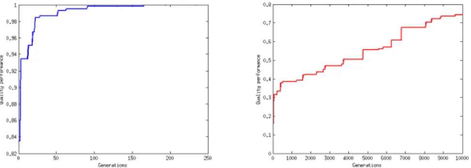
Figure 3 represents the maximum performance attained at each generation of one optimisation for reaching the global maximum of the arena on the left panel and for avoiding “dangerous”zones on the right panel. We can remark that the second task is the most difficult to achieve. Indeed, we observe that the optimisation of reaching the global maximum is perfectly performed in less than 250 generations. However, avoiding “dangerous”zones does not reach the maximum performance at the end of the optimisation (after 10 000 generations).

Fig. 3. Maximum performance reached at each generation of the genetic algorithm for the achievement of one particular task. Left panel: maximum performance for reaching the global maximum of the arena. Right panel: maximum performance for avoiding “dangerous zones”. The achievement of the first task is perfect after a few generations while the achievement of the second task does not reach the maximal performance.

3.2 Combined tasks

Three different learning processes are considered in order to find the best way to train robots for multiple tasks. In the first case, networks learn both tasks si-multaneously giving to the total quality measure an equal weight (named in the following 0.5T1 + 0.5T2). In the second one, robots are first trained to achieve the first task and then both tasks simultaneously (named, T1 → T1+T2) while for the last sequence, it is the second task that is trained before the simulta-neous training (T2 → T1+T2). During the simultasimulta-neous learning, the quality performance is once again the average of the quality measures of T1 and T2. Remark 1. Let us observe that a fourth possible configuration could be used, that is, to consider two smaller networks having inputs only for a given task 4

and then juxtapose the two and link in couple each motor output for each small network, in such a way to get a larger network. Some preliminary results showed that the network obtained by juxtaposition of two smaller ones, each one opti-mised for a task, does not seem to have good performance. In the following we will not consider this fourth case because in our opinion these results need to be further analysed, before any conclusion could be done.

Table 2 presents, for each learning sequence, the mean and standard deviation of the final performance computed from ten independent realisations. The non-parametric hypothesis test of Kruskal-Wallis [7] is considered to evaluate the difference of medians. As the p-value is equal to 0.1232, we accept the null hypothesis, which means that the medians of the three learning sequences seem to be similar on the training set.

Table 2. Mean and standard deviation, on 10 optimisations, of the final maximum performance got for each learning sequence. The total quality measure is calculated as the average of the quality performance of T1 and T2 for all the three learning processes.

Learning process Mean Std 0.5T1 + 0.5T2 0.7295 0.0588

T1 → T1+T2 0.7252 0.0407

T2 → T1+T2 0.7606 0.0606

In order to properly assess the quality of the controllers obtained at the end of the training process, we compare their behaviour using validation sets, i.e., scenarios not present in the set used for the training. We consider different ways of changing the arena. In the first and second validation set, we modify respectively the zones where robots lose energy and the shape of the surface to climb (position of the peak and slope of the surface). In the last set, we perform both modifications. Table 3 presents, for each of these validation sets, the mean and standard deviation of the performance got by the neural networks trained

4 _{More precisely, one network composed by 9 inputs, 5 hidden neurons and 4 outputs,}

has only the inputs able to measure the local heights and the second one, formed by 8 inputs, 5 hidden neurons and 4 outputs, to detect the dangerous zones.

with the different learning sequences. A boxplot of the results obtained for each learning sequence is presented on the right panel of Fig. 4.

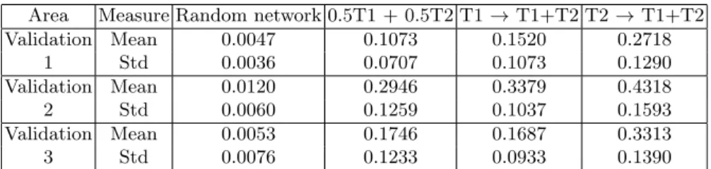
Table 3. Mean and standard deviation of the performance obtained by random neural networks and by the neural networks trained with the different learning sequences on three validation sets, each of them representing a different way to modify the arena.

Area Measure Random network 0.5T1 + 0.5T2 T1 → T1+T2 T2 → T1+T2

Validation Mean 0.0047 0.1073 0.1520 0.2718 1 Std 0.0036 0.0707 0.1073 0.1290 Validation Mean 0.0120 0.2946 0.3379 0.4318 2 Std 0.0060 0.1259 0.1037 0.1593 Validation Mean 0.0053 0.1746 0.1687 0.3313 3 Std 0.0076 0.1233 0.0933 0.1390

The third learning sequence, i.e. the training of the second task followed by the one of both tasks (T2 → T1+T2), seems to be the best way to train robots for multiple tasks. Indeed, the mean performance of this sequence is the highest for each validation set. Moreover, this learning sequence increases the mean perfor-mance by at least 25 % compared to other learning sequences. But we also note that the standard deviation is the highest for this learning process.

To confirm our intuition, we make use of statistical tests whose results are pre-sented on the left panel of Fig. 4. the first test that we use is Kruskal-Wallis in order to check the equality of the three medians. As the p-value is smaller than 0.05, we come to the conclusion that the medians are significantly different. Then, we use the non-parametric Wilcoxon test [7] to evaluate medians by pair. With this test, we observe that sequence 1 and 2 leads to similar medians while the one of sequence 3 is significantly different. Let us remind that the second task, which is first trained in this sequence, is the most difficult to learn. In conclusion, it seems better to train the hardest task before training both tasks simultaneously.

Kruskal-Wallis p-value

3.8281.10−4 < 0.05 Wilcoxon

Seq. 1 Seq. 2 p-value

0.5T1 + 0.5T2 T1 → T1+T2 0.4161 > 0.05 0.5T1 + 0.5T2 T2 → T1+T2 0.0002 < 0.05 T1 → T1+T2 T2 → T1+T2 0.0033 < 0.05

Fig. 4. Analysis of the quality values obtained for the three learning sequences. The performance is evaluated on the validation sets by the optimal networks of 10 optimi-sations. Left panel: hypothesis tests of Kruskal-Wallis and Wilcoxon used to compare the medians of the quality performance. Right panel: boxplot of the quality measures.

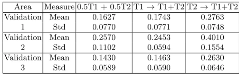
Tables 4 and 5 present the performance associated with the first and the second task, respectively. We can see that the learning sequence T2 → T1+T2 makes it possible to attain the best results because it helps the training process to improve the fitness function of both the tasks.

Table 4. Mean and standard deviation of the task 1 performance obtained by the neural networks trained with the different learning sequences on three validation sets, each of them representing a different way to modify the arena.

Area Measure 0.5T1 + 0.5T2 T1 → T1+T2 T2 → T1+T2 Validation Mean 0.0520 0.1296 0.2672 1 Std 0.0879 0.1441 0.1995 Validation Mean 0.3322 0.4305 0.4625 2 Std 0.1667 0.1736 0.1872 Validation Mean 0.2063 0.1910 0.3937 3 Std 0.2085 0.1401 0.2240

Table 5. Mean and standard deviation of the task 2 performance obtained by the neural networks trained with the different learning sequences on three validation sets, each of them representing a different way to modify the arena.

Area Measure 0.5T1 + 0.5T2 T1 → T1+T2 T2 → T1+T2 Validation Mean 0.1627 0.1743 0.2763 1 Std 0.0770 0.0771 0.0748 Validation Mean 0.2570 0.2453 0.4010 2 Std 0.1102 0.0594 0.1554 Validation Mean 0.1430 0.1463 0.2630 3 Std 0.0589 0.0590 0.0646

4

Discussion

The result of our study about learning sequences is that it seems to be better to learn the hardest task before learning both tasks. This conclusion coincides with the one drawn by Calabretta et al. Nevertheless, far from appearing as a replicate of this study, we flesh out the spectrum of experiments on which the results are valid. Indeed, it is worthwhile to summarise the main differences between our context of study and the one in [3]. Firstly, the two tasks consid-ered in this study are dynamical tasks rather than classification ones. Secondly, both weights and structure of the networks undergo changes during learning. Thirdly, the tasks have separate inputs but common outputs, which is the oppo-site of Calabretta’s experiments. Finally, let us observe that the considered tasks are conflicting and that the weights of the networks do not change in magnitude. Although our study leads to the same conclusion of the one in [3], we can not use the same reason to explain it. Indeed, since the networks and the learning process are different, the neural interference is no longer valid and a different mechanism should be found. To this aim, we study the autocorrelation of our performance landscape [8] for each learning sequence. For this, we perform 10

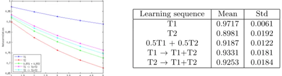
random walks of 10 000 steps in all learning schemes presented before. These walks are executed by random networks for the separate and simultaneous learn-ing of tasks (T1, T2 and 0.5T1 + 0.5T2) while they are performed by networks trained for task 1 and task 2 respectively in the case of successive learning (T1 → T1+T2 and T2 → T1+T2 ). Figure 5 presents the mean of the autocorrelation on the 10 walks for each length from 1 to 5 and for each learning sequence on the left panel and the mean and standard deviation for autocorrelation of length 1 in the table on the right.

Learning sequence Mean Std

T1 0.9717 0.0061

T2 0.8981 0.0192

0.5T1 + 0.5T2 0.9187 0.0122 T1 → T1+T2 0.9331 0.0181 T2 → T1+T2 0.9253 0.0184

Fig. 5. Study of the autocorrelation of the performance landscape. Left panel: mean of the autocorrelation on 10 walks for each length from 1 to 5 and for each learning sequence. Right panel: Mean and standard deviation of the autocorrelation of length 1 for each learning process.

The autocorrelation values explain the marked differences in the final perfor-mance of the robot in the extreme cases, i.e., task 1—the easiest, with the high-est autocorrelation values corresponding to a flatter fitness landscape—and task 2—the hardest, with the lowest values and thus a more rough fitness landscape. Moreover, the learning sequence 0.5T1 + 0.5T2 clearly corresponds to autocorre-lation values just above the ones of T2, but below the others. This explains why this sequence is the worst among the three ones with the compound task. The final high performance attained by the learning sequence T2 → T1+T2 does not seem to find support in the autocorrelation values, which are quite close. How-ever, we must observe that the measure is taken on a landscape corresponding to the final phase of evolution on task 1 (T1 → T1+T2) and task 2 (T2 → T1+T2), respectively. Therefore, at the beginning of the search with the composite fitness (accounting for both the tasks), the autocorrelation of the landscape is strongly influenced by the initial training phase with only one task active. Hence, the landscape autocorrelation in the sequence T2 → T1+T2 heavily depends on the autocorrelation of the landscape for learning task 2, which is the very low. We can conclude that in the T2 → T1+T2, the addition of the fitness component corresponding to task 1 is considerably beneficial to the search process, enabling the genetic algorithm to explore a way smoother landscape, whilst the addition of the task 2 fitness has a dramatically detrimental effect, harming search effec-tiveness.

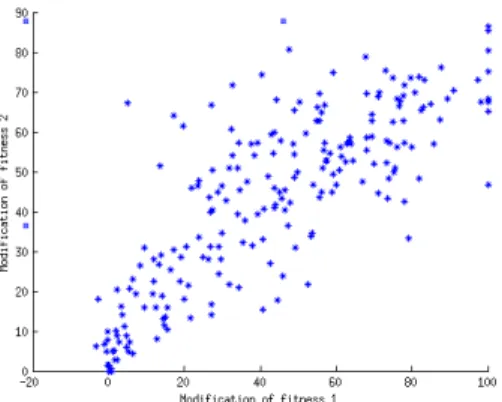
The second point that we discuss is the existence of correlation between the tasks. With this aim, we perform the removal of one hidden neuron at once

and we analyse the modifications of the quality measures. These modifications are shown in Fig. 6 for 10 optimisations of the networks on both tasks simul-taneously. We can observe a linear relation between the modifications, which is confirmed by the correlation coefficient (0.8138). However, can we conclude that neurons that are important for the first task are also important for the second one? Or, is this correlation due to the important number of links in the networks, that we modify too strongly by removing one neuron?

Fig. 6. Relation between the modifications of the two tasks when a hidden neuron is removed from the network. Networks that are considered are the ones obtained after the training on both tasks simultaneously (0.5T1 + 0.5T2).

To provide a first answer to this question we run the same kind of experiments but with a definitive removal of respectively 3 or 5 random chosen hidden nodes before temporarily removing each of the remaining ones and we observed that the correlation between the tasks decreases.

In order to learn more about the topology of our networks and the relations between the two tasks, we need to study the modularity of our networks. Two kinds of modularities can be considered. The first one is a topological modu-larity [9] that can be studied with some community detection methods such as the Louvain method [2] or by using measures of centrality or similarity. In order to analyse the second one, namely the functional modularity, that is to group together neurons that have similar dynamic behaviours, we plan to use some recent information-like indicators [15]. This study will be done in future work.

5

Conclusion

Evolutionary robotics has led to important progress in the domain of artificial cognition. Nevertheless, general results are still lacking about the issue of training a robot controller such that the robot accomplishes multiple tasks. This paper has examined what is the best learning sequence for the training of two tasks with different difficulty. The conclusion of this study has expanded the results brought to light by Calabretta et al. [3] to a more general framework.

In this work, we train robot controllers such that the robot is able to reach the maximum of a surface while avoiding “dangerous”zones where it looses energy. The optimisation is executed both on weights and structure of the networks. Dif-ferent learning sequences are envisaged in order to find the best way for learning multiple tasks.

The learning sequence that has been shown to be appropriate for the learn-ing of conflictlearn-ing multiple tasks is the sequence in which the most difficult task is learnt before the learning of both tasks simultaneously. Contrary to the study of Calabretta, we can not ascribe the difference in the performance to neural interference, because of a different experimental setting. However, a possible ex-planation can come from the study of the autocorrelation of the fitness landscape. The conclusion of this study is promising and supports the claim about the generality of the result, as it extends the application framework with respect to previous works. Further work will address the topology of the networks as well as the relations between the two tasks by the study of the networks modular-ity. This better knowledge of the structure and the tasks relations could lead to important progress in the understanding of learning process.

Acknowledgements

This research used computational resources of the “Plateforme Technologique de Calcul Intensif (PTCI)”located at the University of Namur, Belgium, which is supported by the F.R.S.-FNRS.

This paper presents research results of the Belgian Network DYSCO (Dynamical Systems, Control, and Optimisation), funded by the Interuniversity Attraction Poles Programme, initiated by the Belgian State, Science Policy Office. The scientific responsibility rests with its authors.

References

[1] M.A. Beaumont. Evolution of optimal behaviour in networks of boolean automata. Journal of Theoretical Biology, 165:455–476, 1993.

[2] V. D. Blondel, J-L. Guillaume, R. Lambiotte, and E. Lefebvre. Fast unfolding of communities in large networks. Journal of Statistical Mechanics: Theory and Experiment, 2008(10):P10008, 2008.

[3] R. Calabretta, A. Di Ferdinando, D. Parisi, and F. C. Keil. How to learn multiple tasks. Biological Theory, 3(1):30, 2008.

[4] K. Deb. Multi-Objective Optimization using Evolutionary Algorithms. John Wiley & Sons Ltd, Chichester, 2008.

[5] M. Dorigo and M. Colombetti. Robot Shaping: An Experiment in Behavior Engi-neering. The MIT Press, 1998.

[6] D E Goldberg. Genetic Algorithms in Search, Optimization, and Machine Learn-ing. Addison-Wesley, 1989.

[7] M. Hollander, D. A Wolfe, and E. Chicken. Nonparametric statistical methods, volume 751. John Wiley & Sons, 2013.

[8] H. H. Hoos and T. St¨utzle. Stochastic local search: Foundations & applications. Elsevier, 2004.

[9] N. Kashtan and U. Alon. Spontaneous evolution of modularity and network motifs. Proceedings of the National Academy of Sciences, USA, 102(39):13773– 13778, 2005.

[10] D. MacKay. Information Theory, Inference, and Learning Algorithms. Cambridge University Press, Cambridge, 2005.

[11] D. Nicolay and T. Carletti. Neural networks learning: Some preliminary re-sults on heuristic methods and applications. In A. Perotti and L. Di Caro, edi-tors, DWAI@AI*IA, volume 1126 of CEUR Workshop Proceedings, pages 30–40. CEUR-WS.org, 2013.

[12] S. Nolfi and D. Floreano. Evolutionary robotics. The MIT Press, Cambridge, MA, 2000.

[13] P. Peretto. An introduction to the modeling of neural networks. Alea Saclay. Cambridge University Press, Cambridge, 1992.

[14] R. Rojas. Neural networks: A systematic introduction. Springer, Berlin, 1996. [15] M. Villani, A. Filisetti, S. Benedettini, A. Roli, D. A. Lane, and R. Serra. The

detection of intermediate-level emergent structures and patterns. In Advances in Artificial Life, ECAL, volume 12, pages 372–378, 2013.