A projekt keretében elkészült tananyagok:
Anyagtechnológiák
Materials technology
Anyagtudomány
Áramlástechnikai gépek
CAD tankönyv
CAD book
CAD/CAM/CAE elektronikus példatár
CAM tankönyv
Méréstechnika
Mérnöki optimalizáció
Engineering optimization
Végeselem-analízis
Finite Element Method
Editor:
ÁDÁM KOVÁCS
Authors:ISTVÁN MOHAROS
ISTVÁN OLDAL
ANDRÁS SZEKRÉNYES
FINITE ELEMENT METHODE
Faculty of Mechanical Engineering
Óbuda University
Donát Bánki Faculty of Mechanical and Safety Engineering
Szent István University
Faculty of Mechanical Engineering
and Economics, Faculty of Mechanical Engineering;
István Moharos, Óbuda University, Donát Bánki Faculty of Mechanical and Safety Engineering; István Oldal, Szent István University, Faculty of Mechanical Engineering
READERS: Ágnes Horváthné Varga, István Keppler, Lajos Pomázi, József Uj
Creative Commons NonCommercial-NoDerivs 3.0 (CC BY-NC-ND 3.0)
This work can be reproduced, circulated, published and performed for non-commercial purposes without restriction by indicating the author's name, but it cannot be modified.
ISBN 978-963-687-1
PREPARED UNDER THE EDITORSHIP OF Typotex Publishing House
RESPONSIBLE MANAGER: Zsuzsa Votisky
GRANT:
Made within the framework of the project Nr. TÁMOP-4.1.2-08/2/A/KMR-2009-0029, entitled „KMR Gépészmérnöki Karok informatikai hátterű anyagai és tartalmi kidolgozásai” (KMR information science materials and content elaborations of Faculties of Mechanical Engineering).
KEYWORDS:
Finite Element Method, ANSYS, COSMOS/M, rods, beam, plane stress, plane strain, beam structure, axisymmetric, plate, shell
SUMMARY:
The history of the finite element model, its mathematical foundation and its role in mechanical engineering design are presented. The necessary basic continuummechanical notions and equations for understanding of the method are also discussed. Element types the most commonly used in design (rod, beam, plane, axisymmetric, thin plate, shell) are described. Starting from the principle of total principle energy the derivation of matrix equilibrium equation related to linear elastic bodies discretized in space and the structure of coefficient matrices for different models are shown. In case of beam structures the structure of equation of motion and the method of eigenfrequency calculation are also presented.
1. HISTORY OF FINITE ELEMENT METHOD INCLUDING ITS EVOLUTION, EXTENSION AND ROLE OF APPLICATION IN MECHANICAL ENGINEERING
DESIGN ... 11
1.1.Ancient application ... 11
1.2.History of variation of calculus, basic definitions ... 12
1.2.1. Brachistochrone problem ... 12
1.2.2. Functionals, variations ... 14
1.2.3. Direct method ... 16
1.3.Ritz-method ... 18
1.4.Evolution of modern finite element method ... 20
1.4.1. Force method ... 20
1.4.2. Motion method ... 20
1.5.Finite element method in engineering practice ... 21
1.6.Appendix ... 22
1.6.1. Principals of calculus of variation ... 22
1.6.2. Euler-Lagrange differential equation ... 23
2. FOUNDAMENTAL DEFINITIONS IN CONTINUUM MECHANICS. DIFFERENTIAL EQUATION SYSTEM OF ELASTICITY AND ITS BOUNDARY ELEMENTS PROBLEM. ... 25
2.1.Fundamental definitions in continuum mechanics ... 25
2.2.Differential equation system and boundary element problem of Elasticity ... 33
2.2.1. Equilibrium equations ... 33
2.2.2. Geometric equations ... 36
2.2.3. Constitution equations (material equations) ... 40
2.2.4. Boundary conditions ... 41
2.2.5. Boundary element method ... 42
3. ENERGY THEOREM OF ELASTICITY, CALCULUS OF VARIATION, FINITE ELEMENT METHOD, DETERMINATION OF STIFFNESS EQUATION IN CASE OF CO-PLANAR, TENSED ELEMENT ... 43
3.1.Approximate functions ... 43
3.1.1. Kinematically admissible displacement field ... 43
3.2.Principle of virtual energy ... 44
3.3.Principle of minimum potential energy ... 45
3.4.Principle of Lagrange variation ... 47
3.5.Finite element model based on displacement method ... 48
3.5.1. Introduction of vector fields ... 48
3.5.2. Elasticity problem and the method of solution ... 51
3.5.3. Finite element, approximate displacement field ... 52
3.6.Definition and solution of stiffness matrix in case of co-planar tensed truss element55 3.6.1. Stiffness matrix of 2D, tensed, truss element ... 55
3.6.2. Example ... 60
4. ANALYSIS OF TWO-DIMENSIONAL TRUSSES USING FINITE ELEMENT METHOD BASED PROGRAM SYSTEM ... 64
4.2.Finite elements for modeling beams ... 64
4.2.1. The TRUSS element properties ... 65
4.2.2. Beam Element’s properties ... 66
4.3.Study solution ... 66
4.4.Remarks ... 75
5. TWO-DIMENSIONAL BENT BARS VARIATION PROBLEM, STIFFNESS EQUATIONS AND SOLVING THEM BY FINITE ELEMENT METHOD ... 76
5.1.Two-dimensional bent beam element variation study ... 76
5.2.Solving the problem using finite element method ... 77
5.2.1. The element stiffness matrix ... 78
5.2.2. The entire structure stiffness matrix ... 84
5.2.3. The complete equations system and the solution ... 85
5.3.Remarks ... 86
6. ANALYSIS OF TWO-DIMENSIONAL BENT BARS USING FINITE ELEMENT METHOD BASED PROGRAM SYSTEM ... 87
6.1.Planar beam structures ... 87
6.2.The used finite elements in modeling ... 87
6.2.1. Properties of the BEAM element ... 87
6.2.2. The shear deformation ... 88
6.3.The study solution ... 90
6.4.Remarks ... 104
7. APPLICATION THE PRINCIPLE OF THE MINIMUM POTENTIAL ENERGY IN FIELD OF THREE-DIMENSIONAL BENT BAR ELEMENTS, RITZ METHOD AND FINITE ELEMENT METHOD ... 105
7.1.Three-dimensional bent bars variational problem ... 105
7.2.Solving the problem using finite element method ... 110
7.3.Remarks ... 113
8. ANALYSIS OF THREE-DIMENSIONAL BENT BARS USING FINITE ELEMENT METHOD BASED PROGRAM SYSTEM ... 114
8.1.Three-dimensional beam structures ... 114
8.2.The used finite elements in modeling ... 114
8.2.1. The properties of the BEAM3D elements ... 114
8.2.2. The special properties of BEAM3D elements ... 117
8.3.The study solution ... 119
8.4.Remarks ... 134
9. DYNAMICS OF BEAM STRUCTURES, MASS MATRIX, NATURAL FREQUENCY ANALYSIS ... 135
9.1.Extending of the finite element method ... 135
9.2.Finite element formulation of the elastic bodies' natural oscillation ... 135
9.3.Natural frequency calculation of two-dimensional bar structures using finite element method ... 137
9.3.1. Determination of the element mass matrix ... 138
9.3.2. Element stiffness matrix ... 140
9.3.3. The system total mass and stiffness matrix ... 141
9.4.Remarks ... 143
10. DYNAMIC ANALYSIS OF THREE-DIMENSIONAL BARS, DETERMINATION OF NATURAL FREQUENCY USING PROGRAM SYSTEM BASED ON FINITE ELEMENT METHOD ... 144
10.1. Introduction ... 144
10.2. Properties of the used finite elements ... 144
10.3. The study description ... 144
10.4. The finite element solution of the task ... 146
10.5. Remarks ... 154
11. INTRODUCTION TO PLANE PROBLEMS SUBJECT. APPLICATION OF PLANE STRESS, PLANE STRAIN AND REVOLUTION SYMMETRIC (AXISYMMETRIC) MODELS ... 155
11.1. Basic types of plane problems ... 155
11.2. Equilibrium equation, displacement and deformation ... 155
11.3. Constitutive equations ... 158
11.3.1. Plane stress state ... 158
11.3.2. Plane strain state ... 160
11.4. Basic equations of plane elasticity ... 161
11.4.1. Compatibility equation ... 161
11.4.2. Airy’s stress function ... 162
11.4.3. Navier’s equation ... 162
11.4.4. Boundary value problems ... 163
11.5. Examples for plane stress ... 165
11.5.1. Determination of the traction on the boundaries of a square shape plate ... 165
11.5.2. Analysis of a tangentially loaded plate ... 167
11.6. The governing equation of plane problems using polar coordinates ... 168
11.7. Axisymmetric plane problems ... 172
11.7.1. Solid circular cylinder and thick-walled tube ... 172
11.7.2. Rotating disks ... 175
11.8. Bibliography ... 179
12. MODELING OF PLANE STRESS STATE USING FEM SOFTWARE SYSTEMS. MODELING, ANALYSIS OF PROBLEM EVALUATION ... 180
12.1. Finite element solution of plane problems ... 180
12.2. Linear three node triangle element ... 182
12.2.1. Interpolation of the displacement field ... 182
12.2.2. Calculation of the stiffness matrix ... 185
12.2.3. Definition of the loads ... 186
12.3. Example for the linear triangle element – plane stress state ... 188
12.4. Quadratic six node triangle element ... 197
12.5. Isoparametric four node quadrilateral ... 197
12.5.1. Interpolation of the geometry ... 197
12.5.2. Interpolation of the displacement field ... 201
12.5.3. Calculation of strain components, Jacobi matrix and Jacobi determinant . 201 12.5.4. The importance of the Jacobi determinant, example ... 204
12.5.5. Calculation of the stress field ... 205
12.5.6. Calculation of the stiffness matrix ... 206
12.5.7. Calculation of the force vector ... 207
12.6. Numerical integration, the Gauss rule ... 209
12.6.1. One dimensional Gauss rule ... 210
12.6.2. Two dimensional Gauss rule ... 211
12.7. Example for the isoparametric quadrilateral ... 214
12.9. Bibliography ... 221
13. MODELING OF AXISYMMETRIC STATE BY FEM SOFTWARE SYSTEMS. MODELING, ANALYSIS OF PROBLEM EVALUATION ... 223
13.1. Finite element solution of axisymmetric problems ... 223
13.2. Axisymmetric linear triangle element ... 226
13.3. Example for the application of axisymmetric triangle element ... 228
13.4. Axisymmetric isoparametric quadrilateral element ... 232
13.5. Example for the application of axisymmetric isoparametric quadrilateral element235 13.6. Bibliography ... 243
14. MODELING OF THIN-WALLED SHELLS AND PLATES. INTRODUCTION TO THE THEORY OF SHELL FINITE ELEMENT MODELS ... 244
14.1. Plate and shell theories ... 244
14.2. The basic equations of Kirchhoff plate theory ... 244
14.2.1. Displacement field ... 244
14.2.2. Strain components ... 245
14.2.3. Stress field, forces and moments in the midplane ... 245
14.2.4. The equilibrium and governing equation of thin plates ... 247
14.3. Finite element equations of thin plates ... 250
14.4. Basic equations of the technical theory of thin shells ... 252
14.4.1. Geometrical equations ... 252
14.4.2. Stress resultants and couples, equilibrium equations ... 255
14.4.3. Displacement field, strain components ... 257
14.4.4. Approximations within the technical theory of thin shells ... 258
14.5. Major steps in the finite element modeling of shells ... 259
14.6. Bibliography ... 261
15. MODELING OF IN-PLANE THIN-WALLED SHELLS UNDER IN-PLANE AND TRANSVERSE LOAD BY FINITE ELELEMT METHOD BASED SOFTWARE SYSTEMS ... 262
15.1. Plate elements subjected to bending ... 262
15.2. Triangular plate bending element or Tocher triangle element ... 262
15.3. Example for the application of the Tocher triangle plate element ... 267
15.4. Incompatible rectangular shape plate element ... 270
15.5. Example for the application of the incompatible rectangle shape element ... 274
15.6. Compatible rectangular shape plate element ... 277
15.7. Plates under in-plane and transverse load ... 280
15.8. Bibliography ... 280
16. MODELING OF SPATIAL THIN-WALLED SHELLS BY FINITE ELEMENT METHOD-BASED SOFTWARE SYSTEMS ... 281
16.1. Simple flat shell elements ... 281
16.2. Superposition of the linear triangle and Tocher bending plate elements ... 281
16.3. Example for the combination of the linear triangle and Tocher triangle elements ... 287
16.4. Bibliography ... 294
17. MODELING OF CURVED AND DOUBLY-CURVED SHELLS BY FINITE ELEMENT METHOD BASED SOFTWARE SYSTEMS ... 295
17.1. Curved shell elements ... 295
17.2. Thin-walled cylindrical shell element ... 295
17.3. Axisymmetric shell problems – conical shell element ... 302
17.5. A shell-solid transition element ... 314
17.6. Bibliography ... 315
18. ANALYSIS OF 3D PROBLEMS WITH FINITE ELEMENT BASED PROGRAM SYSTEMS. INTRODUCTION OF 3D ELEMENTS. ... 317
18.1. Hexahedron elements ... 317
18.1.1. Hexahedron element with 8 nodes ... 318
18.1.2. Hexahedron element with 20 nodes ... 320
18.1.3. Hexahedron element with 32 nodes ... 321
18.1.4. Pentagon elements ... 323
18.2. Tetrahedron elements ... 323
18.2.1. Tetrahedron element with 4 nodes ... 326
18.2.2. Tetrahedron element with 10 nodes ... 327
18.2.3. Tetrahedron element with 20 nodes ... 329
18.3. Hierarchic basis functions ... 331
18.4. Definition of stiffness matrix and nodal loads ... 331
18.4.1. Numerical Gauss integration method ... 331
18.4.2. Definition of stiffness matrix in case of 3D elements ... 332
18.4.3. Derivation of nodal loads from distributed force system on volume ... 332
18.4.4. Derivation of nodal loads from distributed force system on surfacel ... 333
19. ANALYSIS OF 3D PROBLEMS WITH FINITE ELEMENT BASED PROGRAM SYSTEMS. APPLICATION OF 3D ELEMENTS. ... 335
19.1. Creation of geometric model ... 335
19.1.1. Editing the original geometry ... 335
19.1.2. Modeling sides and corners ... 336
19.1.3. Modeling unloaded parts ... 336
19.1.4. Modeling symmetric parts ... 337
19.2.1. Defining the mesh ... 338
19.2.2. Influence of element size ... 338
19.2.3. Influence of element type ... 340
19.3. Boundary conditions ... 342
19.3.1. Loads ... 343
19.3.2. Constraints ... 345
20. PRINCIPLES ABOUT MODELING, ACCURACY AND APPLICABILITY. COMPARISON OF DIFFERENT FINITE ELEMENT MODELS, ANALYSIS OF RESULTS. ... 348
20.1. Modeling beams ... 348
20.1.1. Analysis of a beam with circular cross section ... 348
20.1.2. Modeling of thin-walled beams ... 350
20.1.3. Modeling of thin-walled open cross section beams ... 352
20.1.4. Modeling of thick-walled cylinders, tubes ... 358
21. EVALUATION AND APPLICATION OF COMPUTATIONAL RESULT IN DESIGN AND QUALIFICATION RELATED MECHANICAL ENGINEERING TASKS. RELATIONSHIP BETWEEN FINITE ELEMENT METHOD AND STANDARDIZED STRENGHT BASED DESIGN. ... 363
21.1. Precision of Finite Element Method ... 363
21.1.1. Estimation of error in case of h-type approximation ... 365
21.1.2. Calculation of error in case of h-type approximation ... 372
21.1.4. Convergence in singular locations ... 376
21.1.5. Modeling mistakes ... 376
21.2. Evaluation of the calculated results ... 376
21.2.1. Stresses beyond yield strength ... 376
21.2.2. Singular locations ... 377
1.
HISTORY OF FINITE ELEMENT METHOD INCLUDING ITS
EVOLUTION, EXTENSION AND ROLE OF APPLICATION IN
ME-CHANICAL ENGINEERING DESIGN
1.1. Ancient application
Finite elements: complex, and mostly (in case of certain conditions) insolvable problems can be simplified by them. The basic idea is to break up the geometry of the body into finite, sim-ple shaped elements, thus the problem becomes solvable. By this way – instead of applying less but more difficult steps – simple but more mathematical calculation will be carried out in order to find the solution.
Application of discretization on geometrical problems
Arc length and area of a circle (Fig. 1.1)
Volume of a cylinder and sphere,
Other complex geometries.
Figure 1.1: Approximation of the area of the a circle
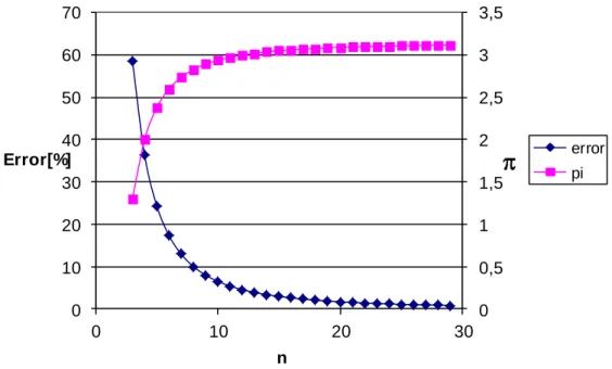
In order to calculate the area of a circle plate, the geometry must be broken up to n identical elements, as it is seen on Figure 1.1.a. The approximated value of, and its error function related to the discretization is shown on Figure 1.2:
n n n 2 360 sin 2 360 cos , and 2 100% 360 sin 2 360 cos n n n Error . a) b)
0 0,5 1 1,5 2 2,5 3 3,5 0 10 20 30 40 50 60 70 0 10 20 30
Error[%] n error piFigure 1.2: Value of π and its error in the function of n discretization
Tsu Ch’ung-Chih, Chinese engineer (A.D 480) determined by the use of rectangles that the approximated value of π is between 3,1415926 and 3,1415927.
1.2. History of variation of calculus, basic definitions
1.2.1. Brachistochrone problem
Bernoulli formed a problem in 1696, which initiated the evolution of variation of calculus in order to find the solution.
The problem: Two points (A and B) are given on a plane. These points are located at
dif-ferent heights and not on the same vertical line. Let us consider co-planar, vertical curves connecting the two points. If a particle is released from point A, without initial velocity and the effect of friction, on which curve would it descend to point B within the shortest time. The question is, whether such a function (among the curves) exists, which allows the particle to complete the motion in the shortest possible time, and if it does, how is it possible to deter-mine it? P1 P2 x y x2 y2
The demanded y function intersects points P and 1 P , thus: 2 0 ) 0 ( y and y(x2) y2 (1.1)
According to the Conservation of Energy:
mgy mv2 2 1 (1.2) The velocity: dt ds v (1.3)
The infinitesimal arc length:
2 2 2dy dx
ds (1.4)
(1.2) simplifying with the mass and substituting (1.3) and (1.4):
gy dt dy dt dx 2 2 2 1 (1.5)
Setting the equation:
gy dx dx dt dy dt dx 2 2 2 (1.6) gy dt dx dx dy 2 1 2 2 (1.7)
By separating the variables, the demanded T time to run the arc length:
2 0 2 2 ' 1 x dx y g y T . (1.8)Let us find that function which satisfies the (1.1) and provides minimum to (1.8). The so-lution is a cycloid: 2 2 1 1 1arcsin 2 ) ( c x x c c x c t y , (1.9)
where c1, c2 constants, and can be determined from (1.1) condition.
This problem – which is practically extremizing a scalar quantity– drew the attention of the variation of calculus and started its evolution.
1.2.2. Functionals, variations
Similar problems as the ,,Brachistochrone” often appear in natural- and social science. We frequently face indexes, quantities which are defined by functions. The simplest example is the solution of an indeterminate integral, which depends on the chosen function. At the same time, an arc length, surface, volume or the potential energy of a beam bears the same mean-ing. These quantities are called as functionals.
An arbitrary set mapped to the set of real numbers is named functional or operator.
It is a specific case of the general mathematic definition, when a set of functions is mapped to the set of real numbers, and named as functional.
Let: f R3 R given function, and yRR possible function, which is
continuous-ly differentiable on its argument yC1[x1,x2] and intersectsP1 (x1,y1), and P2 (x2,y2) points which are fixed at the boundary of the domain:
1 1)
(x y
y , y(x2) y2. (1.10)
Then let us assign all y to:
2 1 ) ( ' ), ( , ] [ x x dx x y x y x f y I (1.11)real number. Thus we can define I as a functional.
In most cases the problem is to extremize the values of the functional. The extreme value can be either absolute or local.
If the I
y functional is valid on the entire argumentum function~yy, andI
y I ~y , then I ~ is absolute minimum.
yIf the I
y functional is only valid on a certain part of the argumentum, andI
y I ~y , then I ~ is local minimum.
yThe classical definition of the variation of calculus is analogue with the calculus. Lagrange introduced the variation – denoted by δ – and defined the rules, similarly as it is in the calcu-lus. Let us examine the classical definition:
The variation of y~ function is y , and we know that y(x1)0 andy(x2)0. y
disap-pears in the x and 1 x points of the domain, while between them is arbitrary. 2 y yy
pro-vides a sum of (permitted) functions, which includes the solution as well. The variation of the functional is defined as:
2 1 x x dx f I . (1.12)The solution of y~ can be obtained if the functional has a minimum. According to the
vari-ation definition 0
I
. (1.13)
This is necessary condition of the extreme value.
In case of a functional-minimum based method the solution of the problem can be defined as an exact or an approximate, which is analogue to the absolute and local minimum theory.
Exact solution, if the function – which provides minimum to the functional – is chosen
among all possible, existing function.
To find that specific function is only possible in very simple cases. In most cases the exact solution cannot be found, since it is neither possible to solve the equations analytically, nor examining infinite functions to see which one provides minimum. Still the problem must be solved even if we are unable to provide the exact solution. Then an approximate solution must be found. x y y x1 x2 P2 P1 y
Approximate solution, if the function – which provides minimum to the functional – is
not chosen among all possible, existing function.
Direct methods were created to find approximate solution. The so called Euler’s broken lines were the elements of Euler’s variation method. This method – by wielding the accesso-ries of modern mathematics – gained attention and became the foundation of the direct me-thods of variation of calculus.
1.2.3. Direct method
The first problem of the variation of calculus was the determination of extremizing functions which provides extreme values to the functional.
Fundamentals of Euler’s method: let us consider the problem analogue with extrema prob-lem of functions which depend on finite variables. Thus permitted functions have finite (n) describing variable, and the integral which is defined as functional (1.11) will be substituted with an approximate value. If n converges to infinite, then the approximate value converges to the value of the integral.
Euler’s solution: the use of linear, continuous ,,Euler’s broken line’’ functions for each part of the domain. Let us divide the
x1, x2
interval to n1 identical part, and give arbitrary real numbers1,...,n. Then the length of the lines:1 1 2 n x x t .
The points of
x1,y1
, x1t,1
, x12t,2
,..., x1nt,n
, x2,y2
are connected with broken lines, and it creates a continuous function which start and end points are fixed in) , ( 1 1 1 x y P andP2 (x2,y2). x y x1 x2 P2 P1 x +it1 i t
Then the (1.13) functional can be modified as: t t t i x f I n i i i i n
1 1 1 1 , , , (1.14)
n1: y 2
.If the approximate value of I functional equals to the extreme value of any Euler’s bro-n
ken line, then in the
x1,y1
, x1t,1
, x12t,2
,..., x1nt,n
, x2,y2
points the deriva-tive: 0 j n I , j1,...,n. (1.15)Let us introduce the partial derivative of a function with respect to the variable denoted by lower index: y f fy : , ' : ' y f fy , …
Then another denotation for the basic function is:
t t j x f f j : 1 ,j,j j 1 Thus:
' ' 1 j y j y j y j n f f t f I . (1.16)Setting the equation of (1.15) and (1.16):
' 1 ' 0 t f f f y j y j j y . (1.17)If n, t0 and the series of the broken lines converges to a two times differentiable
y function, then from (1.17)
0 ) ' , , ( ) ' , , ( f ' x y y dx d y y x fy y , (1.18)
0 ' y f dx d y f . (1.19)
This is a differential equation which belongs to the f basic function and named as Euler-Lagrange differential equation. The solution is y, which provides the minimum of the (1.11) functional. Thus the (1.13) and (1.18) equations mean different definition of an extrama prob-lem in case of a given functional. This equation can be also derived by examining the extrema of a one-parametric sum of functions (1.6. table), however Euler’s broken lines theory is the foundation of the direct methods that is why the classical definition was examined in details.
According to the broken lines let us consider the series of the permitted functions –
de-noted as k– related to the absolute extrema value in the kth steps equals to
k i i i a 0 (1.20)which provides a function in each step. The obtained function series must be examined (if it is convergent) whether its extrema existence is satisfied or not. This method can be used as:
An approximate method for problems in variation of calculus,
If the boundary function has an extreme value and satisfies (1.18), thus the solution of
a differential equation can be transform to a variation problem. This is called as the direct method of variation of calculus.
1.3. Ritz-method
In the Ritz-method, the direct method of variation of calculus is applied to find an approx-imate solution. In contrary with the finite element method, here the complete domain is mod-eled with one function.
Definition: Let n series exist on a norm, anda series on real numbers. n n series is
complete, if to all element there is a
n n
a a11 ...
series, which arbitrary approximates it.
Definition: Let I be a functional, and n series the argumentum of I. Let us consider, that
I minimizable on the linear combination of n set, if:
A linear norm exists, which is part of the argumentum I, and n is complete on it,
All linear combination of n also part of the argumentum of I ,
In all cases of n exists an I minimal element, where n
n i i i I a D n 1 : . (1.21)According to Ritz’s theorem, if a functional can be minimized on the linear combination
of a n set, then I must have a minimal element which is continuous and in that case, yn –
which is the series of the minimal function of I – is the minimizing series of I functional.
Ritz method in elasticity
Let us choose the potential energy of a flexible body as a functional. By the use of n , fi-nite parameter, an approximate function of a kinematically admissible displacement field is created (definitions see at 3.1.1. and 3.3. chapters). According to the theorem of minimum potential energy, the potential energy is minimal in case of real displacement.
The kinematically admissible displacement field is approximated by a function series:
) ,..., , ( ... 1 2 1 1 an n u a a an a u . (1.22)
The derived potential energy includes the same number of n parameter:
) ,..., , (a1 a2 an . (1.23)
The potential energy is a functional, thus its extrema is found in case of
0 (1.24) Thus: 0 ... 2 2 1 1 n n a a a a a a . (1.25)
Since this integral depends on the parameters, the extrema is obtained by the derivation of the potential energy with respect the parameters and equaling to zero:
0 1 a , 0 2 a , …,
0 n
a , thus we obtain a linear algebraic n degree system of equation which provides the
parameters of nseries. Naturally, the function series is arbitrary chosen, the solution is only
approximated. The important element of the method, that the (1.22) displacement field must be kinematically admissible, therefore it would satisfy the kinematic boundary conditions. In case of complex problems, the determination of the functions are quite difficult, thus the me-thod is limited to simple problems. The finite element meme-thod has the advantage to simplify the geometry of the body to simple elements, thus the approximate functions can be found easily.
1.4. Evolution of modern finite element method
1.4.1. Force method
In the early ‘40s the jet planes appeared, and the high terminal and operating velocity de-manded more complex structures, such as the swept and delta wings. The earlier methods to design these special wings appeared to be useless, since the unreliability of the calculation could not be compensated by safety coefficients due to the increasing price of the applied ma-terials, operational costs. A sudden need arose for a reliable and precise calculation method for complex geometries.
Levy applied first the force method, which is based on the classic elasticity that the displacements were calculated from the equilibrium of the forces. He published his first paper about the jet planes with swept wings in 1947. In case of Delta wings problems appeared with the force method, thus another approach had to be used for the solution.
1.4.2. Motion method
Parallel with the force method, other methods – based on the displacements – were being re-searched in order to put it into practice. In 1956, a research group of the Boeing Company – led by Turner – published a problem solved by a new method. The method based on the solu-tion of a stiffness matrix derived from a kinematically admissible displacement, which in-cludes the basics of the current modern finite element method.
In the following decades new solutions were found for 2 and 3D problems, with large dis-placement and various kinds of geometric, material and other non-linearities.
After the recognizing the importance of the analysis of convergence and the parallelism between the matrix equations and elasticity principles, the finite element method was put on a new foundation in the ‘60s, which was called as: calculus of variation.
The new method – which based on the virtual displacement – became almost the ultimate solution earth wide. The problems of applied mathematics and their solutions are still being developed as computer science is constantly evolving.
The finite element method is widely applied on constructional, thermo- and fluid mechan-ical problems, including linear- non-linear and FSI problems as well. Since the computers and the programs rapidly developed they became user-friendly and highly useful tools for the en-gineers. However, the lack of theoretical background resulted inappropriate choice of boun-dary conditions and models, which failed to provide the solution of the real problem.
1.5. Finite element method in engineering practice
The spread of finite element method fundamentally changed the classical process of produc-tion, since it was implemented into the production chain (Fig. 1.6).
Prototípus legyártása
nem felel meg
Gyártás
Tervezés Próbaüzem megfelel
Figure 1.6.: Simplified model of classical production
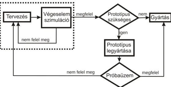
The production and operation of the prototype consumes considering cost during production. These phases require materials, machining, special conditions for the operation test, experi-mental tools and rigs. Naturally, assistance with special skills are also demanded to carry out the production and the test of the prototype. These costs are only balanced if the production has either great volume or the manufactured pieces are simply expensive. This cost is rele-vantly decreased by finite element simulation (Figure 1.7.).
Prototípus legyártása Gyártás Tervezés Próbaüzem megfelel
nem felel meg
Végeselem
szimuláció Prototípus szükséges
megfelel nem felel meg
igen
nem
Figure 1.7.: Finite element aided model of production
The required number of prototypes is reduced by the finite element simulation, and in case the problem can be easily modeled, then the prototype production might be even neglected. In such a case, the mass production can begin and only the zero series must be tested during op-eration.
The simulation provides help during the technological design as well and not only in the strength check. Different software is available to model molding, forging, deep drawing processes, thus the high cost production methods also become cheaper.
We can state that the finite element method – applied in the design – is spread to many fields:
Strength, thermodynamic, fluid, magnetic examination of the piece during normal
operation conditions. This helps to improve the quality of the product and reduce the cost (i.e. reducing weight),
Real-time simulation of the product during the manufacturing process in order to achieve an optimal cost for a proper manufacturing technique,
Simulation of tools, which provides additional information about tool life and optimal
operation conditions.
The finite element method is not only spread in the production, but in other scientific fields as well. Analogously with the manufacturing, the required prototypes and experiments can be greatly reduced, thus the design is cheaper, faster and more precise.
1.6. Appendix
1.6.1. Principals of calculus of variation u function, F F(x,u,u') functional.
The variation of the function or its small scale perturbation: u.
The first variation of the functional:
' ' u u F u u F F , (1.26) Total derivative: ' ' ' du u F du u F dx x F F . (1.27)
In case ofF , 1 F functional the following equations are valid: 2
2 1 2 1 ) (F F F F , (1.28) 2 1 2 1 2 1 ) (F F F F F F , (1.29) 2 2 2 1 2 1 2 1 F F F F F F F , (1.30) F nF Fn n 1 ) ( . (1.31)
It is valid tou function, that:
dx du u dx d , (1.32)
u(x)dx
u(x)dx . (1.33)1.6.2. Euler-Lagrange differential equation
Let f R3 R
a given function (base function), and yRR is an admissible function,
which is continuously derivative along its argumentumyC1[x1,x2], intersects P1 (x1,y1)
and P2 (x2,y2) fixed points on the boundary and valid to the following
state-ments:y(x1) y1, y(x2) y2. Let us assign to all y functions the
2 1 ) ( ' ), ( , ] [ x x dx x y x y x f y I (1.34) real number.Let us find that certain y function to which the I[ y] functional stationer. (In case of
cer-tain conditions it takes on extreme values).
Let RR arbitrary function with fixed points of
0 ) ( ) (x1 x2 , (1.35)
and R real number. Then we can define an R2 Rparametric set of functions:
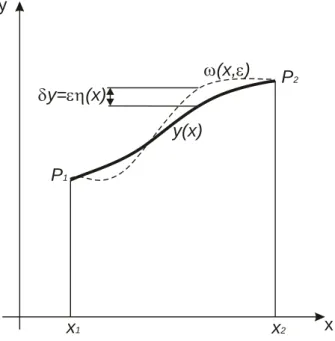
) ( ) ( ) , (x y x x . (1.36) x y (x, ) y= (x) x1 x2 P2 P1 y(x)
Figure 1.8 : Solution of a variation problem and the varied curve
2 1 2 1 ) ( ' ) ( ' ), ( ) ( , ) ( ' ), ( , x x x x dx x x y x x y x f dx x x x f I . (1.37)In case of a given (x) function the I functional only depends on . I() can be only
stationer (satisfying the required boundary conditions), if
0 d dI , (1.38) and 0 . (1.39)
According to the differential rules of the parametric integrals:
0 ' ' ' ' 2 1 2 1 2 1
x x x x x x dx y f dx y f dx y f y f d dI . (1.40)We apply the partial integration rule on ' ' y f :
2 1 2 1 2 1 ' ' ' ' x x x x x x dx y f dx d y f dx y f . (1.41)The first member of the right side of (1.41) is zero according to (1.35), thus substituting into (1.40): 0 ' 2 1
x x dx y f dx d y f . (1.42)Since is necessary, the integral can only be zero, if
0 ' y f dx d y f .
2.
FOUNDAMENTAL DEFINITIONS IN CONTINUUM
MECHANICS. DIFFERENTIAL EQUATION SYSTEM OF ELASTICITY
AND ITS BOUNDARY ELEMENTS PROBLEM.
2.1. Fundamental definitions in continuum mechanics
Model: simplified approximation of reality, which behaves similarly as the examined phenomena.
In order to solve problems in the strength of materials certain models are required as:
geometrical,
material-,
mechanical (load, constraints).
Geometrical models – according to their dimensions – can be:
0D: particle model, all the geometrical dimensions are neglected,
1D: if two dimensions can be neglected compared to one. Classical beam-truss
elements and line elements used in finite element method.
2D: if one dimension can be neglected compared to the two others. Plates and
membranes.
3D: None of its dimensions can be neglected. Although this statement does not always
include the complete geometry, since some parts can be still simplified in the mechanical point of view. Only those parts must be ignored which significantly increase the computation but less relevantly the precise of the result.
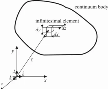
Continuum model: A continuum model can be divided up to finite (or infinite) elements
and described by continuous (and continuously derivative) functions. The points of the continuum body can be appointed by a position vector
k z j y i x r (2.1)
in a given coordinate system.
Infinitesimal element: an infinitesimally (arbitrarily) small element of a continuum body,
depending on the model it can be an infinitesimal mass or volume.
Rigid body: the length between two arbitrarily chosen points of a rigid body is always
constant, independently the magnitude of the load.
Elastic body: the body is capable to deform elastically. The length between its points
changes depending on the applied load.
Linear elastic material model: the relationship between the load and deformation is
linear.
Non-linear elastic material model: the relationship between the load and deformation is
non-linear.
Plastic material model: the subject remains deformed after the removal of the load and
does not regain its original form. Several plastic models exist depending on the dominancy of linear, non-linear, elastic or plastic properties.
Figure 2.2.: Material models
Isotropic material: the behavior of the material does not depend on the direction; all
properties are the same independently any arbitrarily direction.
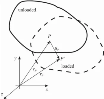
Displacement vector: the difference vector between P and P points. The points ' represent an arbitrary point of an elastic body before- and after applying a load, thus the original – undeformed – and deformed states.
k w j v i u uP P P P (2.2)
Displacement field: displacement vector of all points of the body in the function of the
position vector (2.1). k r w j r v i r u r u( ) ( ) ( ) ( ) (2.3)
Small displacement: the displacement of the points of the body is irrelevantly small
compared to the geometrical dimensions of the body.
Kinematic boundary conditions: the given (or admissible) displacements of the body. Dynamic boundary conditions: the given (or admissible) load of the body.
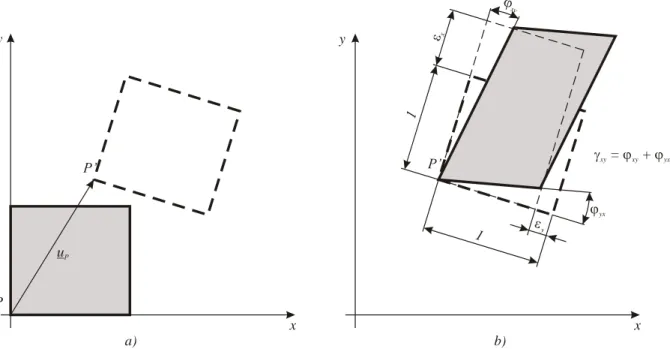
Deformation: the proportional displacement of the points of the body (related to a unit
length).
Strain: the gradient of length of vector,
Torsion of angle: the angle gradient of perpendicular axes (Figure 2.4.b.), the torsion
of angle is always symmetric.
The rigid body motion is not taken into account (Figure 2.4.a.).
Deformation vector: this vector describes the displacement of a given unit vector. Defining it
byi ,,j k unit vectors (trieder):
k j i ax x xy xz 2 1 2 1 , (2.4) k j i ay yx y yz 2 1 2 1 , (2.5) k j i az zx zy z 2 1 2 1 , (2.6) where, zx xz zy yz yx xy , , .
The property of the vector coordinates:
Specific strains: x,y,z properties without dimensions, 0
, the length increases,
0
, the length decreases.
Angle torsion: xy,yz,xz the dimension is in radian 0
, the angle decreases,
0
, the angle increases.
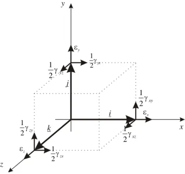
Deformation state: the sum of the deformation vectors related to all directions in a given
point. Possible description: infinitesimal unit cube with deformation vectors, deformation tensor, Mohr circle.
P x y x P’ P’ y 1 y yx xy = xy +yx a) b)
Tensor: linear, homogenous vector-vector function. Description is possible with dyadic
form or a matrix defined in a given coordinate system.
Deformation tensor: It describes the deformation state of any point of an elastic body by
assigning the deformation vector of a given direction to an arbitrary direction. Description is possible with three vectors in matrix or dyadic form in a given coordinate system.
In dyadic form: k a j a i ax y z . (2.7) In matrix form: z yz xz zy y xy zx yx x 2 1 2 1 2 1 2 1 2 1 2 1 , (2.8)
The deformation vector coordinates of x, y, z, are in the columns.
The an deformation vector related to an arbitrarily chosen n direction is defined as:
n
an . (2.9)
Deformation tensor field: the deformation field of all points of the body in the function
of position vector. y z x x i j k y z xy 2 1 xz 2 1 yx 2 1 yz 2 1 zx 2 1 zy 2 1
r r r r r r r r r r z yz xz zy y xy zx yx x 2 1 2 1 2 1 2 1 2 1 2 1 (2.10)Stress: The intensity of the internal force system distributed on the internal face of the
body. Dimension: Pa
m N
1
1 2 .
Stress vector: the stress is defined by a stress vector. The n
stress vector of a dA surface related to an arbitrarily chosen n direction is defined as:
dA F d
n
. (2.11)
On a given surface, the normal coordinate of the stress vector is named as
normal stress, and denoted by: .
0 , in case of tension, 0 , in case of compression.
The coordinate of the stress vector which is parallel with the surface is
named as shear stress, and denoted as: .
The stress vectors defined byi ,,j k unit vectors on a given surface:
k j i xy xz x x , (2.12) k j i y yz yx y , (2.13) k j i zy z zx z , (2.14) where, zx xz zy yz yx xy , , .
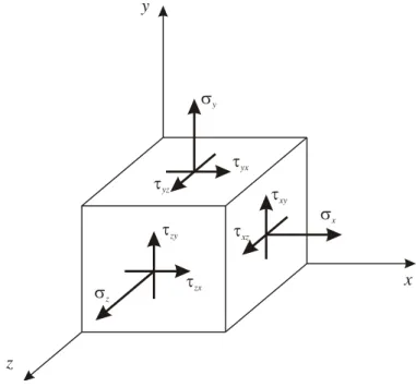
Stress state: the sum of the stress vectors related to all directions in a given point.
Stress tensor: It describes the stress state of any point of an elastic body by assigning the
stress vector of a given direction to an arbitrary direction. Description is possible with three vectors in matrix or dyadic form in a given coordinate system.
In dyadic form: k j i z y x . (2.15) In matrix form: z yz xz zy y xy zx yx x . (2.16) n
stress vector defined to an n direction:
n
n
. (2.17)
Stress tensor: the stress field of all points of the body in the function of position vector.
r r r r r r r r r r z yz xz zy y xy zx yx x (2.18)The element index of the stress- and strain tensor can be used in a reversed order not only
y z x x xz xy yx zy yz zx y z
as it was presented earlier.
The work of a force: a force acted along a rd displacement carries out an Fdr
infinitesimal work (see the geometric description of the scalar multiplication on the Figure 2.7; the force is multiplied by the force directed component of the displacement). The work carried out along a finite displacement is the sum of the infinitesimal works.
r d r F W r r
2 1 ) ( (2.19)Internal energy: (deformation energy) the energy of the internal forces
dV U V xz xz yz yz xy xy z z y y x x
2 1 (Linear case) (2.20)The internal energy can be derived from the double product of the stress and deformation tensor: dV U V
2 1 (2.21)Hamilton operator: (Nabla operator) is a vector, which coordinates are special orders to
execute the partial differentiations of the given directions. In a Descartes coordinate system:
k z j y i x . (2.22) r1 x y z r r2 r+dr F F dr drF dW= d =Frcos =FdrF r F
In cylindrical (polar) coordinate system: z R e z e R e R 1 . (2.23)
2.2. Differential equation system and boundary element problem of Elasticity
2.2.1. Equilibrium equations
The equilibrium equations describe the relationship between the q(r) distributed force system
acting on a volume and the
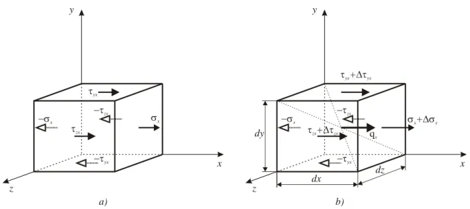
r stress field tensor.If an arbitrarily chosen infinitesimal body inside of a body is in steady state, then the external (Figure 2.8.a.) and internal (Figure 2.8.b.) forces are in equilibrium. By investigating the forces along the x axis (Figure 2.9.a.), it is clearly obvious: if no external forces are acting upon the body, then the internal forces (stresses) have equal magnitude and opposite senses on the proper sides of the body. The change is caused by the external distributed force system acting on the volume. Stress is an internal force distributed on a surface, thus it must be recalculated onto the infinitesimal cube. xappears on the dydz surface of the cube, and it
turns to be a force system acting on a volume if it is divided by dx side length. Similarly, zx
shear stress must be divided bydz, while yx must be divided by dy side length. Then, all
forces acting upon the infinitesimal body along the x axis are in equilibrium:
0 x yx yx yx zx zx zx x x x q dy dy dz dz dx dx . (2.24) y z dV x r i j k q(r) a) y z x x xz xy yx zy yz zx y z b)
The gradient of the stresses can be described by the partial derivative of the given direction: dx x x x , dz z zx zx , dy y yx yx
, which are substituted into (2.24)
we obtain: 0 x zx yx x q z y x . (2.25)
Analogously to the earlier, the other two directions:
0 y zy y xy q z y x , (2.26) 0 z z yz xz q z y x . (2.27)
The (2.25)-(2.27) equations are the so called equilibrium equations in Descartes coordinate system.
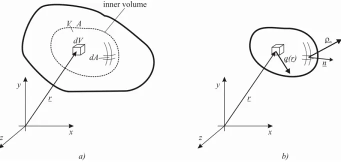
In order to define generally the equilibrium equations let us consider a V volume inside of a body similarly to Figure 2.10.
a) b) y z x x yx zx zx yx x y z x x+ x yx+ yx zx+ zx zx yx x qx dx dz dy
The infinitesimal force acting on a dV volume of the infinitesimal body:
dV q F
d .
The infinitesimal force acting on a dA surface, and calculated from the
n stress vector: dA n dA F d n .
The V internal body is in equilibrium, thus the sum of the forces acting on the surface and
the volume are zero:
A V dA n dV q F 0 . (2.28)According to the Gauss-Ostrogradsky integral-transformation theorem:
dV dA n V A
.Substituting Gauss-Ostrogradsky into (2.28):
dV dV q V V
0 ,Setting the separated parts of the equation into one integral:
q
dV V
0 (2.29)Since the V volume is arbitrarily chosen, thus the (2.29) equation is only valid if the integral is zero. This is the equilibrium equation of elasticity.
0 q . (2.30) 2.2.2. Geometric equations
The geometric (kinematic) equations define the relationship between the u(r) displacement
field and the
r deformation tensor field. On Figure 2.8, the deformation of an infinitesimalcube is presented in the xy plane of a Descartes coordinate system.
Let us neglect the rigid-body motion, and let us investigate the relative displacement between
point P andQ . By plotting P and P points on each other, the gradient of PQ length is the '
'
QQ vector, which is denoted by du duidv jdwk infinitesimal displacement
vector. It has two coordinates in a plan, namely du and dv . Both coordinated can be broken
up into two parts: dudux duy, dvdvy dvx.
x
du : from the strain of dx side (in the function of x ),
y
du : from the strain of dy side (in the function of y),), thus
0 dx du x u x u x u x y x and dy du y u y u y u x y y 0 . P x y xy = xy +yx du dx dv dy yx xy xy dux duy duy dvx dvy dvx Q’ P’ Q du
y
dv : from the strain of dy side (in the function of y ),
x
dv : from the strain of dx side (in the function of x ), thus
0 dx dv x v x v x v x y x and dy dv y v y v y v x y y 0 .
According to Figure 2.11, the strains are:
dx dux x , dy dvy y ,
While the torsion of angle is:
dy du dx dv dy du dx dvx y x y yx xy xy arctan arctan .
By the use of the partial derivatives related to the displacement vector:
x u x , y v y , y u x v yx xy .
This calculation can be carried out on all planes, which result the geometric equations in a Descartes coordinate system:
x u x , y v y , z w z , (2.31) y u x v yx xy , y w z v zy yz , z u x w zx xz . (2.32)
The geometric equations can be defined in a general form. Let us investigate the position of two points on an elastic body before and after applying an external load on it. The distance
between the two points – in the undeformed state – isdr dxidyjdzk.
According to the definition of deformation the gradient of displacement between the two points has to be examined and described.
The difference of the two points is defined by the relative displacement of P and Q points: P P Q u u u u u .
Thus the displacement ofQ :
u u
u P . (2.33)
Let us approximate the u
x,y,z
displacement function in the close environment of P byapplying a Taylor-series on P point:
dx u du x u dz z u dy y u dx x u u r u P P P P P P ... 2 1 2 2 2 . (2.34)Figure 2.12.: Displacement and deformation
P P’ uP Q Q’ uQ= u dr d ’r uP u dr
From (2.33) and (2.34) can be derived that in the close environment of P the difference and the derivative are approximately equal. In case of small displacement the higher derivatives can be neglected:
dz z u dy y u dx x u u d u P P P .
Taking into accountdxidr, dy jdr, dz kdr equilibriums, and the group theory between the scalar and dyadic product a
bc ab
c, the infinitesimal gradient of the displacement field is:
k dr z u j y u i x u r d k z u r d j y u r d i x u u d P P P P P P .By the use of the Hamilton operator:
u
dr ud . (2.35)
Where T
u
the derivative tensor of the displacement field, which can be divided toa symmetric and anti-symmetric (skew-symmetric) tensors.
T T
T T
u u
u u
T T T T 2 1 2 1 2 1 2 1The symmetric part describes the deformation of the infinitesimal body while the anti-symmetric describes the rotation of the infinitesimal body. Thus the deformation tensor derived from the displacement field is described as:
uu
2 1
(2.36)
Equation (2.36) is the so-called geometric equation.
The identical scalar equations of the tensor form are described in a Descartes coordinate system as it was mentioned earlier in (2.31) and (2.32) equations.
The other type of geometric equations is the to so-called Saint-Venant compatibility equation: 0 .
The compatibility is also related to the neighbor infinitesimal elements, since the material is continuous, and the displacement of the neighbor elements have to be identical as well.
2.2.3. Constitution equations (material equations)
The constitutional- or material equations determine the relationship between the stress and strain state. The behavior of the material on Figure 2.2 can be described as linear, and the Hooke law is suitable to describe to phenomena. In case of single axis stress state, the simple Hooke law can define the relationship between the strain and the stress: E, where E (Young-modulus, elasticity modulus) is the coefficient between the stress and strain. In case of tension or compression, the stress has only one principle direction thus component, but strain appears in two directions as it is seen on Figure 2.14. There is positive elongation in the material along the axis of tension, but in the same time, it contracts perpendicularly. The relationship between the elongation and the contraction is described by the dimensionless Poisson-coefficient: y z x.
In case of multi-axes stress state, the relationship between the stress and strain state can be only described with a tensor equation, the so-called general Hooke law. The law has two isotropic form to linear, elastic materials:
G 1E 2 1 2 , (2.37) E G 1 1 2 1 . (2.38) where,
G: shear elastic modulus, which can be calculated as: E2G
1
,E : unit matrix,
1 1,
: the first scalar invariant of the tensors, (the sum of the main row?).
The scalar equations with respect to (2.37) material equations:
x y
1 1