Soil cracks detection by 3D electrical resistivity.

HAL Id: hal-00079734

https://hal-insu.archives-ouvertes.fr/hal-00079734

HAL is a multi-disciplinary open access archive for the deposit and dissemination of sci-entific research documents, whether they are pub-lished or not. The documents may come from teaching and research institutions in France or abroad, or from public or private research centers.

L’archive ouverte pluridisciplinaire HAL, est destinée au dépôt et à la diffusion de documents scientifiques de niveau recherche, publiés ou non, émanant des établissements d’enseignement et de recherche français ou étrangers, des laboratoires publics ou privés.

Soil cracks detection by 3D electrical resistivity.

Anatja Samouëlian, Isabelle Cousin, Guy Richard, Ary Bruand, Alain

Tabbagh

To cite this version:

Anatja Samouëlian, Isabelle Cousin, Guy Richard, Ary Bruand, Alain Tabbagh. Soil cracks detection by 3D electrical resistivity.. 9th European Meeting of Environmental and Engineering Geophysics, 2003, Prague, Czech Republic. 5 p. �hal-00079734�

Section headings : Cavity and void detection

2

SOIL CRACKS DETECTION BY 3D ELECTRICAL RESISTIVITY

4

Samouëlian, A.1, Cousin, I.1, Richard, G. 2, Bruand, A., 4Tabbagh, A. 3 5

(1) INRA, Unité de Science du Sol, BP 20619, 45166 Ardon France 6

(2) INRA Unité d’Agronomie, rue Fernand Christ, 02007 Laon France 7

(3) UMR 7619 « Sisyphe », Case 105, 4 place Jussieu, 75005 Paris 8

(4) UMR 6113 ISTO, 1a rue de la férollerie, 45071 Orléans Cedex 2 9

10

Introduction 11

Soil cracks, whose formation are associated to natural climate phenomena such as swelling 12

and shrinking, play an important role in water and gas transfers. Up to now, their 3D structure 13

was characterised either by serial sections (Cousin, 1996) which is a destructive technique or 14

X-ray tomography (Macedo et al., 1998) which is applicable on limited size sample. Three-15

dimensional electrical resistivity prospecting enables now to monitor crack development and 16

to characterise their geometry without any destruction of the medium under study. Three-17

dimensional electrical resistivity surveys are commonly gathered by a network of in-line 18

survey arrays, such as Wenner, Schlummberg, or dipole-dipole (Xu and Noel, 1993; Zhou et 19

al., 2002). As emphasized by Meheni et al. (1996) the resulting apparent resistivity maps are 20

often different depending on the array orientation related to an electrical discontinuity. 21

Chambers et al. (2002) underline that in heterogeneous medium 3D electrical resistivity 22

model resolution was sensitive to electrode configuration orientation. Indeed asymmetric 23

bodies or anisotropic material exhibit different behaviours depending on whether the current 24

passes through them in one direction or in another (Scollar et al., 1990). It would be all the 25

more true for medium having very contrasted resistivities like cracking soil. In that case the 26

electrical current does not encounter the same resistance when it passes perpendicular or 27

parallel to the resistant bodies. Measurements of apparent resistivity depend then on the 28

location and orientation of the current source relative to the body under study (Bibby, 1986). 29

Studies conducted by Habberjam and Watkins (1967) emphasized that the square array 30

provide a measurement of resistivity less orientationally dependent than that given by a in-31

line array investigation. 32

Intending to lead a more 3D accurate inversion, we have chosen to focus our attention on a 33

3D electrical resistivity data acquisition. We present here a three-dimensional electrical 34

survey carried out by a square array quadripole for characterising the soil cracks network 35

developing during a desiccation period. 36

37

Material and Method 38

The experiment was conducted on a loess soil block (26 by 30 by 40 cm3 in size). It exhibited 39

a massive structure resulting from severe compaction after wheels traffic in wet conditions. At 40

sampling, the initial volumetric water content was 0.43 cm3cm-3. It was then let to dry for 18 41

days. During this time, the soil porosity increased: cracks appeared at the soil surface and 42

spread toward the soil at depth. 43

The electrical resistivity measurements were done by 64 Cu/CuSO4 electrodes arranged on 8

44

lines by 8 columns as shown in fig.1. The electrode spacing “a” was chosen equal to 3 cm, 45

which was a priori supposed to achieve the detection of millimetre cracks as shown in a 46

previous experiment at the centimetre scale (Samouëlian et al., 2003). The number of data 47

was 280 measurements spread out 7 pseudo-depths. For each array, 2 measurements were 48

done, the current being injected in 2 perpendicular directions. The respective apparent 49

electrical resistivity measurements were noted ρ0° and ρ90°, if ρ0° and ρ90° are equal, the

50

sounding medium is homogenous with no electrical heterogeneity. 51 52 y (α=90°) 53 54 x (α=0°) 55

Figure 1 : Square array configuration and possible modes of connection

56 57

Results and discussion 58

Global description of the 3D apparent resistivity data at the end of the experiment 59

Resulting from the two-array orientation α=0° and α=90°, we calculated an apparent 60

anisotropic index (AI) defined by equation [1] : [1] 61

62

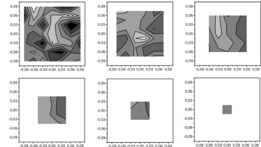
The determination of electrical anisotropy index was suitable as it may enhance the presence 63

of heterogeneities. It permitted also to summarize for each pseudo-depth the electrical 64

resistivity measurements on a single map (figure 2). The AI revealed major anisotropic zones 65

linked to elevated or low AI values. As expected, they were rather located at the soil surface 66

than at depth: the apparent anisotropic index varied from 0.07 to 9.63 in the first pseudo-67

depth, in the second and third pseudo depths the variation decreased slightly 0.38 to 0.5 for 68

the minimum values and 7.54 to 4.64 for the maximum values. The deeper pseudo-depths, 69

four, five, and six, did not exhibit large variations, because the size of the array was probably 70

larger than the crack extents. 71 72 73 74 75 76 77 78 79 80 81 82 83 84

Figure 2 : Spatial distribution of the Anisotropic Index (AI) at the final stage

85 86

Cracks detection for the first pseudo-depth 87

AI can be considered as an indicator of cracks detection. For the first pseudo-depth, we

88

determined the relation between AI, the mean crack width and the crack orientation for each 89

elementary area. When the crack width was greater than 1 mm, two groups could be 90

distinguished related to the thresholds Icinf and Icsup corresponding respectively to 0.42 and 91

to 3.14. When the relation Icinf < AI <Icsup was verified, the related zone was considered as a 92

no cracking zone; when it was not verified, the related zone was considered as a cracking 93

zone (figure 3). The crack preferential orientation (α = 0° or α = 90°) could also be deduce by 94

the AI value. When it was larger (resp. smaller) than 1, the preferential orientation was α = 95

90° (resp. 0°). Moreover one can notice that cracks that do not cross the MN in-line 96

measurements have an AI value between Icinf and Icsup. 97

98

Figure 3 : Crack detection and orientation for the first pseudo-depth evaluated by

99 ° ° = 90 0 ρ ρ AI 1 2 4 3 1 2 4 3 _{Electrode position 1 2 3 4} α = 0 A B M N α = π N A B M 0,20 0,39 0,75 1,5 2,8 5,5 0,20 0,39 0,75 1,5 2,8 5,5 -0,09 -0,06 -0,03 0,00 0,03 0,06 0,09 -0,09 -0,06 -0,03 0,00 0,03 0,06 0,09 -0,09 -0,06 -0,03 0,00 0,03 0,06 0,09 -0,09 -0,06 -0,03 0,00 0,03 0,06 0,09 -0,09 -0,06 -0,03 0,00 0,03 0,06 0,09 -0,09 -0,06 -0,03 0,00 0,03 0,06 0,09 -0,09 -0,06 -0,03 0,00 0,03 0,06 0,09 -0,09 -0,06 -0,03 0,00 0,03 0,06 0,09 -0,09 -0,06 -0,03 0,00 0,03 0,06 0,09 -0,09 -0,06 -0,03 0,00 0,03 0,06 0,09 -0,09 -0,06 -0,03 0,00 0,03 0,06 0,09 -0,09 -0,06 -0,03 0,00 0,03 0,06 0,09

represented the cracking area, respectively with cracks preferential orientation 0° and 90°

101

Cracks detection of the all the pseudo-depth 102

a) Calculation of a new index 103

The apparent anisotropy index, AI, presented previously can be used as an indicator of 104

discontinuities like cracks yielding both position and orientation. Nevertheless it is directly 105

calculated by the mean experimental data and as a consequence, the thresholds values given in 106

this paper cannot be generalized to another dataset that would be obtained either on another 107

soil or in different experimental conditions. Thus, we have calculated a second index. To look 108

for the preferential anisotropic orientation, we searched the α-array orientation corresponding 109

to the maximum apparent resistivity values also called αmax-array orientation. The primary

110

data set was transformed into a calculated data set with the help of the rotational tensor R 111

expressed in the equation [2]. 112 ⎟⎟ ⎠ ⎞ ⎜⎜ ⎝ ⎛ − = α α α α cos sin sin cos R [2] 113

Thus a calculated data set was obtained by the equation [3] : 114 ⎟⎟ ⎠ ⎞ ⎜⎜ ⎝ ⎛ = ⎟⎟ ⎠ ⎞ ⎜⎜ ⎝ ⎛ ° ° ° + 90 0 90

ρ

ρ

ρ

ρ

where : ρα and ρ α+90° were the calculated data set obtained for α value varying by 5° steps

116

between 0° and 90°. The rotational tensor highlighted particular features such as the position 117

and orientation of a resistivity discontinuity. 118

b) Calculation of the αmax values on the experimental dataset

119

As summarized in table [1], the distance between the minimum and maximum values of the 120

αmax-array orientation decreased as the pseudo-depth increased. Moreover the values were

121

converging to α=45°, corresponding to a medium without electrical heterogeneities. 122

123

PP1 PP2 PP3 PP4 PP5 PP6 Mini 5 10 10 20 35 45 Max 85 70 65 65 65 50

Table 1 Extremes values of αmax-array orientation.

124

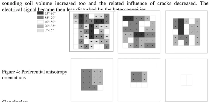
The figure 4 exhibits the spatial distribution of the αmax. For the first pseudo-depth, the α

125

values ranging between 40 and 50 corresponded to the elementary area where Icinf < AI 126

<Icsup. They were associated with an isotropic medium. The α values ranging in the interval 127

0-35 and 55-90 were associated with an anisotropic medium, corresponding to the cracks 128

network. Between the first and the second pseudo-depths, the electrical heterogeneities 129

orientation were preserved or shifted to 45° but never inverted. Depending on the quadripole 130

position the cracks larger than 1mm were detected. Cracks spread out the soil depth with a 131

preferential orientation initiated from the surface. One can also supposed that as the mean 132

crack width increased the corresponding crack depth increased too. For the third pseudo-depth 133

we focused only on the crack mean width larger than 1 mm. Only the triple point was then 134

partially recorded. The crack oriented at 90° was the best detected. As observed at the soil 135

surface, the mean width of this crack nevertheless was the highest: 2.57 mm. The following 136

pseudo-depths four, five, and six displayed an orientation α converging to 45°. 137

In summarize, the studied soil depth does not exhibit any electrical anisotropy and the 138

cracking zone was mainly located at the surface. With an inter-electrode spacing of 3cm, 139

cracks of 1mm width were detected at the soil surface. When the inter-electrode spacing 140

increased from a to 2a (second pseudo-depth), only the major cracks were distinguished. The 141

widest cracks were detected until the third pseudo-depth. As the pseudo-depth increased, the 142

sounding soil volume increased too and the related influence of cracks decreased. The 143

electrical signal became then less disturbed by the heterogeneities. 144 145 146 147 148 149 150 151 152 153

Figure 4: Preferential anisotropy

154 orientations 155 156 157 158 Conclusion 159

These results indicated that electrical resistivity measurement was as expected dependent on 160

the electrical heterogeneities and the variation of signal was even detectable at this scale. The 161

Icinf and Icsup thresholds resulting of the anisotropic index AI and the αmax-array orientation

162

are two methods useful for detecting electrical heterogeneities. The first one was calculated 163

for a specific electrical device, related to a specific soil texture and experimental condition. 164

Nevertheless they can be applied to electrical acquisition corresponding to the temporal 165

monitoring of the desiccation experiment. The second method required time for calculation 166

but presented the advantage to be generalisable to the whole soil volume. The calculation of 167

these 2 indexes gives ideas on the structure of the medium prior to the data inversion. 168

Nevertheless for the both method, cracks oriented near α=45° or cracks who do not cross the 169

in-line measurement MN were not detected. One suggestion is to collect the electrical 170

measurement for in-line measurement along diagonal, which would also increase the 171

acquisition time of about 20 min. 172

173

References : 174

Bibby, H. M. 1986. Analysis of multiple-source bipole-quadripole resistivity surveys using the

175

apparent resistivity tensor. Geophysics 51: 972-983.

176

Chambers, J. E., R. D. Oglivy, O. Kuras, J. C. Cripps and P. I. Meldrum. 2002. 3D electrical imaging

177

of known targets at a controlled environmental test site. Environmental Geology 41: 690-704.

178

Cousin, I. 1996. Reconstruction 3D par coupes sériées et transport de gaz dans un milieu poreux.

179

Application à l'étude d'un sol argilo-limoneux, Reconstruction 3D par coupes sériées et

180

transport de gaz dans un milieu poreux. Application à l'étude d'un sol argilo-limoneux.

181

Université d'Orléans.

182

Habberjam, G. M. and G. E. Watkins. 1967. The use of a square configuration in resistivity

183

prospecting. Geophysical Prospecting 15: 445-467.

184

Macedo, A., S. Crestana and C. M. P. Vaz. 1998. X-ray microtomography to investigate thin layers of

185

soil clod. Soil & Tillage Research 49: 249-253.

186

Meheni, Y., R. Guérin, Y. Benderitter and A. Tabbagh. 1996. Subsurface DC resistivity mapping :

187

approximate 1-D interpretation. Journal of Applied Geophysics 34: 255-270.

188

Samouëlian, A., I. Cousin, G. Richard, A. Tabbagh and A. Bruand. 2003. Electrical resistivity imaging

189

for detecting soil cracking at the centimetric scale. Soil Science Society Journal of America.in

190

press

191

Scollar, I., A. Tabbagh, A. Hesse and I. Herzog. 1990. Archaeological prospecting and remote sensing.

192

Xu, B. and M. Noel. 1993. On the completeness of data sets with multielectrode systems for electrical

193

resistivity survey. Geophysical Prospecting 41: 791-801.

194 75°-90° 55°-70° 40°-50° 20°-35° 0°-15°

Zhou, Q. Y., J. Shimada and A. Sato. 2002. Temporal variations of the three-dimensional rainfall infiltration 195

process in heterogeneous soil. Water Resources Research 38: 1-16. 196