HAL Id: hal-01871975
https://hal.archives-ouvertes.fr/hal-01871975
Submitted on 17 Nov 2020
HAL is a multi-disciplinary open access
archive for the deposit and dissemination of
sci-entific research documents, whether they are
pub-lished or not. The documents may come from
teaching and research institutions in France or
abroad, or from public or private research centers.
L’archive ouverte pluridisciplinaire HAL, est
destinée au dépôt et à la diffusion de documents
scientifiques de niveau recherche, publiés ou non,
émanant des établissements d’enseignement et de
recherche français ou étrangers, des laboratoires
publics ou privés.
The X-ray catalog of spectroscopically identified
Galactic O stars: Investigating the dependence of X-ray
luminosity on stellar and wind parameters
A. Nebot Gomez-Moran, L.M. Oskinova
To cite this version:
A. Nebot Gomez-Moran, L.M. Oskinova. The X-ray catalog of spectroscopically identified Galactic
O stars: Investigating the dependence of X-ray luminosity on stellar and wind parameters.
As-tron.Astrophys., 2018, 620, pp.A89. �10.1051/0004-6361/201833453�. �hal-01871975�
https://doi.org/10.1051/0004-6361/201833453 c ESO 2018
Astronomy
&
Astrophysics
The X-ray catalog of spectroscopically identified Galactic O stars
Investigating the dependence of X-ray luminosity on stellar and wind parameters
?A. Nebot Gómez-Morán
1and L. M. Oskinova
2,31 Observatoire Astronomique de Strasbourg, Université de Strasbourg, CNRS, UMR 7550, 11 rue de l’Université, 67000 Strasbourg, France
e-mail: ada.nebot@astro.unistra.fr
2 Institute of Physics and Astronomy, University of Potsdam, 14476 Potsdam, Germany e-mail: lida@astro.physik.uni-potsdam.de
3 Department of Astronomy, Kazan Federal University, Kremlevskaya Str 18, Kazan, Russia
Received 18 May 2018/ Accepted 3 August 2018
ABSTRACT
The X-ray emission of O-type stars was first discovered in the early days of the Einstein satellite. Since then many different surveys have confirmed that the ratio of X-ray to bolometric luminosity in O-type stars is roughly constant, but there is a paucity of studies that account for detailed information on spectral and wind properties of O-stars. Recently a significant sample of O stars within our Galaxy was spectroscopically identified and presented in the Galactic O-Star Spectroscopic Survey (GOSS). At the same time, a large high-fidelity catalog of X-ray sources detected by the XMM-Newton X-ray telescope was released. Here we present the X-ray catalog of O stars with known spectral types and investigate the dependence of their X-ray properties on spectral type as well as stellar and wind parameters. We find that, among the GOSS sample, 127 O-stars have a unique XMM-Newton source counterpart and a Gaia data release 2 (DR2) association. Terminal velocities are known for a subsample of 35 of these stars. We confirm that the X-ray luminosities of dwarf and giant O stars correlate with their bolometric luminosity. For the subsample of O stars with measure terminal velocities we find that the X-ray luminosities of dwarf and giant O stars also correlate with wind parameters. However, we find that these correlations break down for supergiant stars. Moreover, we show that supergiant stars are systematically harder in X-rays compared to giant and dwarf O-type stars. We find that the X-ray luminosity depends on spectral type, but seems to be independent of whether the stars are single or in a binary system. Finally, we show that the distribution of log(LX/Lbol) in our sample stars is non-Gaussian, with the peak of the distribution at log(LX/Lbol) ≈ −6.6.
Key words. stars: massive – X-rays: stars
1. Introduction
Since the era of the Einstein X-ray telescope (0.2–4.0 keV) it is known that O-type stars emit X-rays (Harnden et al. 1979). Based on the initial sample of 16 OB stars detected by Einstein,Long & White(1980) noted that their X-ray luminos-ity correlates with bolometric luminosluminos-ity as LX ∼ 10−6 ... −8Lbol. Pallavicini et al.(1981) extended the study to 35 stars with spec-tral types in the range from O4 to A9 and concluded that the ratio of X-ray to bolometric luminosity is roughly constant (LX≈ (1.4 ± 0.3) × 10−7Lbol), breaking down for spectral types later than A5. Later on, Schmitt et al. (1985) showed that the log(LX/Lbol) ∼ −7 correlation does not hold for A-type stars breaking down already at spectral type B5. Chlebowski et al. (1989) presented “The Einstein X-ray Observatory Catalog of O-type stars”. The catalog contains 289 stars with 89 detections and 176 upper limits. It was found that X-ray luminosities of O stars are in the range LX≈ 10−5.44 ... −7.35Lbol.
The ROSAT telescope performed an all-sky X-ray survey (RASS,Voges et al. 1999,2000) in the 0.2–2.4 keV energy band and detected many OB-type stars, confirming the LX∝ Lbol corre-? The X-ray catalog is only available at the CDS via anonymous ftp
tocdsarc.u-strasbg.fr(130.79.128.5) or viahttp://cdsarc.
u-strasbg.fr/viz-bin/qcat?J/A+A/620/A89
lation (e.g.,Motch et al. 1997).Berghoefer et al.(1997) demon-strated that this correlation flattens considerably below Lbol ≈ 1038erg s−1, that is, for mid- and late-type B stars. Since then, the LX ∝ Lbol relation was often revisited and confirmed by many independent studies of OB-stars in clusters and in the field.
With the advent of modern X-ray telescopes XMM-Newton and Chandra, with their broad spectral response (0.2–12.0 keV) and high spatial resolution, the interest in X-ray properties of O stars was once more renewed. Oskinova(2005) verified the log(LX/Lbol) correlation selectively, distinguishing between binary and single stars. A linear regression analysis of a sample of spectroscopic binaries showed a correlation LX ≈ 10−7Lbol. It was found that while binary stars are more X-ray luminous than single ones, the correlations between X-ray and bolomet-ric luminosities are similar for both groups. Great effort has been made to study massive star populations in individual clusters (e.g., Moffat et al. 2002;Wolk et al. 2006).Sana et al.(2006) observed the open cluster NGC 6231 using XMM-Newton. Based on a rather small sample of 12 O stars they found a much lower scatter than previous studies (log(LX/Lbol)= −6.91 ± 0.15) and showed that the LX∝ Lbolrelation is dominated by soft X-ray emission – the dispersion becomes larger for radiation above 2.5 keV.
X-ray emission from a large number of O-stars in the Carina Nebula cluster was studied byNazé et al.(2011). Using Chandra observations of 60 O stars in this region, a ratio of
Open Access article,published by EDP Sciences, under the terms of the Creative Commons Attribution License (http://creativecommons.org/licenses/by/4.0),
log(LX/Lbol)= −7.26 ± 0.21 was determined. The spectral types were collected from the literature as presented in the contempo-raneousSkiff(2014) catalog. Interestingly, using XMM-Newton observations of the same region, Antokhin et al. (2008) deter-mined log(LX/Lbol)= −6.58±0.79.Nazé et al.(2011) explained the discrepancy by the different reddening laws and bolometric luminosities assigned to O-stars in these studies.
An X-ray catalog of OB-stars was presented byNazé(2009). They cross-correlated the XMM-Newton Serendipitous Source Catalogue: 2XMMi-DR3(Watson et al. 2009) and the all-sky cat-alog of Galactic OB stars, which contains ∼16 000 known or “rea-sonably suspected” OB stars (Reed 2003). Approximately 300 OB stars were found to have an X-ray counterpart. Confirming previous studies,Nazé(2009) showed that X-ray fluxes of O stars are well correlated with their bolometric fluxes. However, the scat-ter was found to be comparable to that of the RASS studies, that is, much larger than in individual clusters. The average ratio between X-ray (in the 0.5–10.0 keV band) and bolometric fluxes for O-stars was found to be log(LX/Lbol)= −6.45 ± 0.51. Although theReed(2003) catalog of OB stars is a valuable resource, it is heterogeneous by nature, harvesting data from the SIMBAD data-base1, and might contain dubious spectral classifications.
While significant effort firmly established an LX ∝ Lbol correlation for O stars, its origin is still unknown. A standard explanation of X-ray emission from O stars is the presence of plasma heated by shocks intrinsic to radiatively driven stellar winds (Lucy & White 1980;Owocki et al. 1988;Feldmeier et al. 1997). The X-ray luminosity is therefore expected to correlate with stellar wind parameters. One of the most detailed and care-ful analyses to date was performed by Sciortino et al.(1990), who investigated correlations between X-ray luminosity and stellar and wind parameters based on a large sample of O stars detected by the Einstein observatory. They found that LX corre-lates well with mass, the Eddington factor (that describes rela-tive influence of radiation pressure with respect to gravity), Lbol, wind momentum ( ˙M3∞), and kinetic wind luminosity (Lkin), but only weakly with mass-loss rate ( ˙M) and with terminal wind velocity (3∞). Moreover,Sciortino et al.(1990) found that none of these parameters alone can account for the observed disper-sion in LX, but that a combination of Lbol, 3∞ and ˙Mis needed. Motivated by the well-known correlation of LXwith rotation rate in solar-type stars, Sciortino et al. (1990) searched for similar correlations in hot stars but could not find any evidence.
Alternative and still speculative explanations for X-ray emis-sion from O stars invoke stellar magnetism. In this case, hot X-ray-emitting plasma could be associated with stellar spots (e.g., Waldron & Cassinelli 2007). The presence of such mag-netic structures in normal stars is gaining support both the-oretically and observationally (Cantiello & Braithwaite 2011; Ramiaramanantsoa et al. 2014).
The aim of the study presented in this paper is to build a homogeneous catalog of X-ray emitting O stars and to study the dependence of their X-ray emission with stellar and wind proper-ties. The time is now ripe for such a study. The Galactic O-Star Spectroscopic Survey (GOSS) by Sota et al. (2011, 2014) and Maíz Apellániz et al.(2016) is now available. GOSS consists of more than 590 O stars with spectral types homogeneously deter-mined from optical spectroscopy. It is complete down to mag-nitude B = 8 mag. As noted bySota et al. (2014), the previous studies were subject to discrepancies in spectral type determina-tions which can lead to errors deriving parameters that depend on spectral types (and propagate to X-ray studies). The X-ray
1 Wenger et al.(2000).
catalog we present in this paper is limited to stars from the GOSS sample for the sake of consistency.
The release of the GOSS coincides with an on-going improvement and expansion of The XMM-Newton Serendipitous Source Catalogue. In this paper we consider GOSS stars with X-ray counterparts in the latest XMM-Newton catalog at the time of writing. We do not include the information from other X-ray surveys and telescopes in order to study the homogeneous X-ray sample representative for the O star population within our Galaxy. The catalog we present here incorporates distances based on the parallaxes included in the Gaia second data release (DR2).
The paper is structured as follows: in Sect.2we describe the X-ray, optical, and infrared associations. Determinations of stel-lar and X-ray parameters are described in Sects.3and4, respec-tively. Correlations between X-ray and wind parameters are discussed in Sect.5, and conclusions are drawn in Sect.6.
2. The X-ray, optical, and infrared associations of GOSS and the resulting catalog
The XMM-Newton satellite has been operating since 2000 (Jansen et al. 2001). There are five X-ray instruments on board: the three European Photon Imaging Cameras (EPIC), and two Reflection Grating Spectrometers (RGS; Strüder et al. 2001; Turner et al. 2001; den Herder et al. 2001). Among the three EPIC cameras, one is equipped with a pn detector and two with Metal Oxide Semi-conductor CCD arrays (MOS cameras). These cover the energy range from 0.2 to 12 keV, with an energy resolution E/∆E ≈ 50 at 6.5 keV and with a position accuracy better than 300(90% confidence radius). The catalog we present here is limited to X-ray sources detected by the PN camera.
Thanks to the XMM-Newton large field of view and its high sensitivity, in each pointed observation up to 100 sources are detected serendipitously (Rosen et al. 2016). Since 2003 the XMM-NewtonSurvey Science Center has been compiling infor-mation on serendipitously detected X-ray sources and releasing it to the community in the form of catalogs.
The most recent catalog, released in July 2016, is the 3XMM-DR7; it contains 727 790 detections for 499 266 unique sources, covering a sky area of about 1032 square degrees. The median flux in the total photon energy band (0.2–12 keV) is ∼1.9 × 10⁻¹⁴erg cm−2s−1; in the soft energy band (0.2–2 keV) the median flux is ∼6 × 10⁻¹⁵erg cm−2s−1, and in the hard band (2–12 keV) it is ∼8 × 10⁻¹⁵erg cm−2s−1. About 23% of the sources have total fluxes below 1 × 10⁻¹⁴erg cm−2s−1.
To find X-ray counterparts of GOSS stars, their optical positions were cross-matched with the 3XMM-DR7 catalog. We looked for all possible X-ray counterparts within a 3.4σ search radius, where σ is the combined positional error of the X-ray sources and the optical position of the O stars: σ = q
(σX)2+ (σopt)2. Here σX and σopt are the X-ray and optical positional errors respectively and σopt = 100is assumed.
Thanks to the good angular resolution of XMM-Newton, the source confusion is low – there are only a few cases where two O stars are unresolved in X-rays (e.g., HD 37742 and HD 37743 both have positions compatible with 3XMM J054045.5–015633), or where a star has two possible X-ray associations and we thus cannot decide which one is the true counterpart (e.g., Cyg OB2-22 A is compatible with both
3XMM J203308.7+411316 and 3XMM J203308.8+411318).
We visually inspected these cases, but concluded that O star and X-ray source cannot be associated unambiguously. After
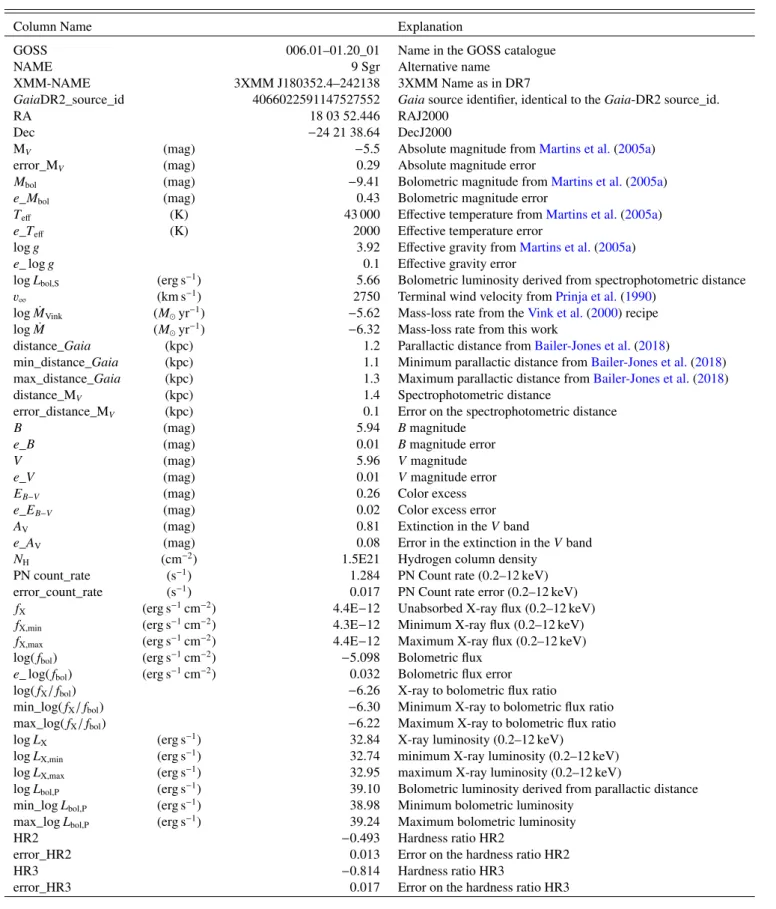
Table 1. An example of entry to the GOSXMM catalog and column descriptions.
Column Name Explanation
GOSS 006.01–01.20_01 Name in the GOSS catalogue
NAME 9 Sgr Alternative name
XMM-NAME 3XMM J180352.4–242138 3XMM Name as in DR7
GaiaDR2_source_id 4066022591147527552 Gaiasource identifier, identical to the Gaia-DR2 source_id.
RA 18 03 52.446 RAJ2000
Dec −24 21 38.64 DecJ2000
MV (mag) −5.5 Absolute magnitude fromMartins et al.(2005a)
error_MV (mag) 0.29 Absolute magnitude error
Mbol (mag) −9.41 Bolometric magnitude fromMartins et al.(2005a)
e_Mbol (mag) 0.43 Bolometric magnitude error
Teff (K) 43 000 Effective temperature fromMartins et al.(2005a)
e_Teff (K) 2000 Effective temperature error
log g 3.92 Effective gravity fromMartins et al.(2005a)
e_ log g 0.1 Effective gravity error
log Lbol,S (erg s−1) 5.66 Bolometric luminosity derived from spectrophotometric distance
3∞ (km s−1) 2750 Terminal wind velocity fromPrinja et al.(1990)
log ˙MVink (M yr−1) −5.62 Mass-loss rate from theVink et al.(2000) recipe
log ˙M (M yr−1) −6.32 Mass-loss rate from this work
distance_Gaia (kpc) 1.2 Parallactic distance fromBailer-Jones et al.(2018)
min_distance_Gaia (kpc) 1.1 Minimum parallactic distance fromBailer-Jones et al.(2018)
max_distance_Gaia (kpc) 1.3 Maximum parallactic distance fromBailer-Jones et al.(2018)
distance_MV (kpc) 1.4 Spectrophotometric distance
error_distance_MV (kpc) 0.1 Error on the spectrophotometric distance
B (mag) 5.94 Bmagnitude
e_B (mag) 0.01 Bmagnitude error
V (mag) 5.96 Vmagnitude
e_V (mag) 0.01 Vmagnitude error
EB−V (mag) 0.26 Color excess
e_EB−V (mag) 0.02 Color excess error
AV (mag) 0.81 Extinction in the V band
e_AV (mag) 0.08 Error in the extinction in the V band
NH (cm−2) 1.5E21 Hydrogen column density
PN count_rate (s−1) 1.284 PN Count rate (0.2–12 keV)
error_count_rate (s−1) 0.017 PN Count rate error (0.2–12 keV)
fX (erg s−1cm−2) 4.4E−12 Unabsorbed X-ray flux (0.2–12 keV)
fX,min (erg s−1cm−2) 4.3E−12 Minimum X-ray flux (0.2–12 keV)
fX,max (erg s−1cm−2) 4.4E−12 Maximum X-ray flux (0.2–12 keV)
log( fbol) (erg s−1cm−2) −5.098 Bolometric flux
e_ log( fbol) (erg s−1cm−2) 0.032 Bolometric flux error
log( fX/ fbol) −6.26 X-ray to bolometric flux ratio
min_log( fX/ fbol) −6.30 Minimum X-ray to bolometric flux ratio
max_log( fX/ fbol) −6.22 Maximum X-ray to bolometric flux ratio
log LX (erg s−1) 32.84 X-ray luminosity (0.2–12 keV)
log LX,min (erg s−1) 32.74 minimum X-ray luminosity (0.2–12 keV)
log LX,max (erg s−1) 32.95 maximum X-ray luminosity (0.2–12 keV)
log Lbol,P (erg s−1) 39.10 Bolometric luminosity derived from parallactic distance
min_log Lbol,P (erg s−1) 38.98 Minimum bolometric luminosity
max_log Lbol,P (erg s−1) 39.24 Maximum bolometric luminosity
HR2 −0.493 Hardness ratio HR2
error_HR2 0.013 Error on the hardness ratio HR2
HR3 −0.814 Hardness ratio HR3
error_HR3 0.017 Error on the hardness ratio HR3
discarding these objects, our final sample contains 135 stars from the GOSS uniquely associated with a 3XMM-DR7 X-ray source. As a next step we collected the optical and infrared pho-tometry for our sample stars. Our sample catalog was cross-matched with the GSC2.3.2 and the 2MASS Point Source Catalogs (2MASS-PSC). The former is an all sky catalog based
on the all-sky photographic surveys from the Palomar and UK Schmidt telescopes (DSS), while the latter is an all sky survey covering approximately the 4 to 16 magnitude range in three bands (J, H and Ks;Cutri et al. 2003). Except for HD 93128, all our sample stars have counterparts within 100 in the GSC2.3.2 and the 2MASS-PSC catalogs.
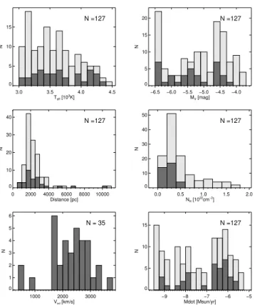
3.0 3.5 4.0 4.5 Teff [10 3 K] 0 5 10 15 N N =127 −6.5 −6.0 −5.5 −5.0 −4.5 −4.0 MV [mag] 0 5 10 15 20 N N =127 0 2000 4000 6000 8000 10000 Distance [pc] 0 10 20 30 40 N N =127 0.0 0.5 1.0 1.5 2.0 NH [10 22cm−2] 0 10 20 30 40 50 N N =127 1000 2000 3000 Vinf [km/s] 0 1 2 3 4 5 6 N N = 35 −9 −8 −7 −6 −5 Mdot [Msun/yr] 0 5 10 15 N N =127
Fig. 1.Histograms showing distributions of stellar parameters for
O-stars in our catalog. From left to right and from top to bottom: effective temperatures, absolute magnitudes, parallactic distances, neutral hydro-gen column densities, stellar wind velocities, and mass-loss rates for the whole sample (127 O stars shown in light gray), and for stars with known terminal velocities (35 stars shown in dark gray).
We exclude HD 93128 from the follow up study since it is located in a crowded field and its photometry is not reli-able, as well as the known high-mass X-ray binaries HD 153919 and LM Vel (Liu et al. 2006;Martínez-Núñez et al. 2017). This reduces our sample to 132 O stars detected with the XMM-NewtonPN camera and uniquely identified.
The full sample of our stars is presented in a table that is accessible in electronic form via the VizieR database2. Table1
shows an example of the parameters provided for each star in our catalog, which includes distances, X-ray, and stellar properties.
3. Stellar parameters
All our sample stars have well determined spectral types. This provides the basis for assigning fundamental parameters to each object. To estimate stellar wind parameters we use an empiric approach. We collect stellar wind parameters from the most recent literature for a sub-sample of our objects, and extrapo-late them to the rest of our sample stars. Figure 1 shows the distribution of the effective temperatures, absolute magnitudes, distances, neutral hydrogen column densities, stellar wind veloc-ities, and mass-loss rates for our sample stars.
3.1. Fundamental stellar parameters
Stellar effective temperatures, log(g), masses, radii and abso-lute magnitudes are assigned to each sample star according to its spectral type using the calibrations from Martins et al.
2 Ochsenbein et al.(2000).
(2005a). Since in this work the tabulated values are limited to luminosity classes V, III, and I, the values for luminos-ity classes IV and II were interpolated. For luminosluminos-ity classes Ia, Ib, and Iab, we assumed absolute magnitudes and e ffec-tive temperatures of supergiant stars. The peak in the abso-lute magnitude distribution seen in Fig. 1 at about −6.4 mag corresponds to O supergiant stars. To estimate errors on stel-lar parameters we assumed an uncertainty on the spectral subtype of ±1, we then determined the corresponding stel-lar parameters and fixed errors to the maximum difference between these determined stellar parameters; for example, σTeff,SpT= max(|Teff ,SpT− Teff ,SpT−1|, |Teff ,SpT− Teff ,SpT+1|). For estimat-ing σlog(g) we performed a similar analysis but assumestimat-ing an uncertainty on the luminosity class of one subclass.
Among the sample of O stars studied here, 38 sources are known to be spectroscopic binaries (Sota et al. 2014). For those cases we display the spectral type of the primary stars. Three sources are known to be magnetic: θ1Ori, HD 57682, and CPD -59 2629 (Donati et al. 2002; Grunhut et al. 2009; Nazé et al. 2014).
3.2. Extinction
Extinction was calculated using color excesses EB−V, EJ−Ks, and
EH−Ks in the optical and in the infrared. The intrinsic colors are
from Martins & Plez (2006). In the optical we calculated the extinction using the relation AV= RV× EB−V with RV= 3.1. In the infrared we used the extinction relations AK= 0.67 × EJ−Ks and AK= 1.82 × EH−KsfromIndebetouw et al.(2005). Then, the
extinction relation AK= 0.114 × AV (Cardelli et al. 1989) pro-vides an alternative way to estimate AV.
For a set of O stars in common with Jenkins (2009) we compared the color excess EB−V and found that, in general, the values we derive here agree well withJenkins(2009). We also compared the optical excesses obtained from the infrared colors. Although we find a good general agreement, the scatter is larger than when using optical colors only. Therefore to estimate the extinction for our program stars we use EB−V as derived from optical photometry.
There are various relations in the literature that link the neu-tral hydrogen column density to the color excess, which range from NH ∼ 1 × 10²¹× EB−Vcm−2to NH ∼ 9 × 10²¹× EB−Vcm−2 (Predehl & Schmitt 1995;Gudennavar et al. 2012;Liszt 2014). In this work we adopt NH= 5.6×10²¹× EB−Vcm−2(Bohlin et al. 1978). In Sect.4.1we consider in detail how this choice affects the estimates of X-ray fluxes of our sample stars.
For two objects (υ Ori and 15 Mon A) the estimated NH is very low. We set NHfor both stars equal to a minimum value of 1018cm−2.
3.3. Distance
The distances to our sample stars were estimated by using both the spectrophotometric and the parallactic methods.
We started by estimating distances from the absolute visual magnitudes derived using bolometric corrections and the pho-tometry of our program stars. The V magnitudes were corrected for the extinction (see Sect. 3.2) and the errors on the spec-trophotometric distances were derived by propagating the errors on magnitudes and extinction.
As a next step, we searched the extended Gaia DR2 cata-log (Bailer-Jones et al. 2018), and found that the parallactic dis-tances are estimated for 127 of our sample stars. These were compared with the spectrophotometric distances we derived.
Reassuringly, the spectrophotometric distances agree well with the parallactic ones. Therefore, in the following we use the Gaia DR2 parallactic distances.
While most of the GOSS sources are within 4 kpc, six sources are estimated to be at larger distances: CPD -59 2600 (estimated distance d = 4.9 kpc) is a member of the open cluster Cl Trumpler 16 for which distances in the literature range from 2 to 5.4 kpc (Mel’Nik & Dambis 2009;Pandey et al. 2010). HD 168076 AB (estimated distance d = 5.1 kpc), is a member of the open cluster M 16 at a distance of 1.7 kpc (Kharchenko et al. 2005). HD 159176 (estimated distance d = 6.6 kpc) and HD 93403 (estimated distance d = 10.2 kpc) are found at distances of 1 and 2.4 kpc, respectively, according to Megier et al. (2009). Finally, for LS 4067 AB (estimated dis-tance d = 10.7 kpc) and ALS 18 769 (estimated distance d = 5.5 kpc), we found no distances in the literature.
3.4. Terminal wind velocities and mass-loss rates
The O star winds are radiatively driven (Castor et al. 1975). While grasping the fundamental physics, currently the stel-lar wind theory has limited predictive power. At present, it is not yet possible to theoretically calibrate stellar wind parame-ters in dependence on spectral types. In this situation, different approaches to estimating wind parameters for a large sample of O stars are possible. First, a full multi-wavelength spectroscopic analysis of each star in a sample could yield their stellar and wind properties. This method is impractical due to, for example, observational challenges. Besides, any stellar atmosphere model used for spectral analysis has its own limitations. Second, the fundamental stellar parameters could be used as input for the-oretical recipes predicting wind velocities and mass-loss rates. This is the easiest and therefore most commonly used option – convenient routines are publicly available (Vink et al. 2000). In Table 1 we list the theoretical mass-loss rates for each star in our sample (log ˙MVink). However, there are notable discrepan-cies between the empirically measured mass-loss rates and those predicted by the theoretical recipes (e.g.,Fullerton et al. 2006). Especially dramatic is the situation for late O-dwarfs, where the models fail (Muijres et al. 2012). Such stars constitute a signif-icant part of our sample. Third, a semi-empirical approach that builds on existing measurements is a practical way to estimate wind parameters for a large number of stars. From UV spec-troscopy, stellar wind velocities are securely measured for 35 stars of our sample. Furthermore, recent spectroscopic analyses using sophisticated stellar atmosphere models were performed for 25 stars in our sample (see Table2). Importantly, these stars belong to different spectral types and were analyzed with differ-ent independdiffer-ent stellar atmosphere models. Hence, the number of empirically well studied stars is sufficiently large to establish an empirical calibration of wind properties that show a dency on spectral type. We choose this option to study the depen-dence of X-ray luminosity on stellar wind parameters.
Using UV spectra of resonance lines obtained by the Inter-national Ultraviolet Explorer,Prinja et al.(1990) measured the terminal velocity in a large number of OB-type star winds3;
among them 35 belong to our sample. Their wind veloci-ties are typically above ∼1000 km s−1. Winds of two stars, HD 93521 (3∞∼ 490 km s−1) and θ1Ori (3∞∼ 580 km s−1), are unusually slow. Another object with a comparably slow wind is HD 152408 (3∞= 955 km s−1). Interestingly, while θ1Or is a 3 We note that the errors on the velocity measurements are not provided byPrinja et al.(1990).
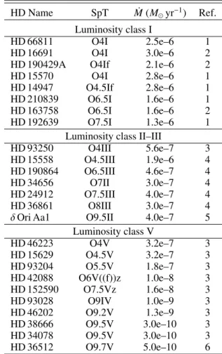
Table 2. Stellar mass-loss rates of O type stars collected from the literature.
HD Name SpT M˙ (M yr−1) Ref.
Luminosity class I
HD 66811 O4I 2.5e–6 1
HD 16691 O4I 3.0e–6 2
HD 190429A O4If 2.1e–6 2
HD 15570 O4I 2.8e–6 1
HD 14947 O4.5If 2.8e–6 1
HD 210839 O6.5I 1.6e–6 1
HD 163758 O6.5I 1.6e–6 2
HD 192639 O7.5I 1.3e–6 1
Luminosity class II–III
HD 93250 O4III 5.6e–7 3 HD 15558 O4.5III 1.9e–6 4 HD 190864 O6.5III 4.6e–7 4 HD 34656 O7II 3.0e–7 4 HD 24912 O7.5III 4.0e–7 4 HD 36861 O8III 3.0e–7 4
δ Ori Aa1 O9.5II 4.0e–7 5
Luminosity class V HD 46223 O4V 3.2e–7 3 HD 15629 O4.5V 3.2e–7 3 HD 93204 O5.5V 1.8e–7 3 HD 42088 O6V((f))z 1.0e–8 3 HD 152590 O7.5Vz 1.6e–8 3 HD 93028 O9IV 1.0e–9 3 HD 46202 O9.2V 1.3e–9 3 HD 38666 O9.5V 3.0e–10 3 HD 34078 O9.5V 3.0e–10 3 HD 36512 O9.7V 5.0e–10 6
Notes. An interested reader is strongly encouraged to consult original papers for details of the spectroscopic analyses.
References. (1) Šurlan et al. (2013); (2) Bouret et al. (2012); (3)
Martins et al.(2005a); (4)Repolust et al.(2004), note that the mass-loss
rates in the table are reduced by a facor of 3; (5)Shenar et al.(2015);
(6)Shenar et al.(2017).
well-known magnetic star, the search for magnetic fields in HD 93521 and HD 152408 did not reveal any (Grunhut et al. 2017;Schöller et al. 2017).
As illustrated in Fig.2, terminal velocity decreases with stel-lar spectral type since stars with lower effective temperatures tend to have lower escape velocities (Prinja et al. 1990). While the stellar wind theory predicts a relationship between the termi-nal velocity and the photospheric escape velocity (Abbott 1978; Lamers & Cassinelli 1999), the scatter seen in Fig.2implies that the situation in real objects may be more complicated, further justifying our empirical approach.
Although only 35 stars have measured terminal velocities, they cover the whole range of possible stellar parameters (see Fig.1), and therefore can be taken as representative of the whole sample.
While stellar wind velocities could be directly measured from UV spectra, measuring mass-loss rates typically requires the model fitting of spectral lines. The errors on the mea-sured mass-loss rates are largely systematic, reflecting the limitations of the applied models. Presently, the most sophisti-cated stellar atmosphere models do not rely on the assumption of local-thermodynamical equilibrium (LTE; i.e., are non-LTE), include line-blanketing, and account for wind clumping (e.g.,
O4 O5 O6 O7 O8 O9 Spectral subtype 0 1000 2000 3000 4000 Vinf [km/s] I,II III IV V
Fig. 2.Terminal wind velocities (fromPrinja et al. 1990) as a function
of the spectral type for O stars of different luminosity classes (see leg-end, the asterisk denotes a known magnetic star).
Hillier & Miller 1998; Hamann & Gräfener 2003; Puls et al. 2005).
We collected literature where the mass-loss rates of our sam-ple stars are obtained from spectroscopic analyses done with advanced model atmospheres. To the best of our knowledge, we found such analyses for 25 O stars in our sample. Each of these models has its own way of describing the effects of wind clumping. The mass-loss rates are compiled in Table2and are the face values from the corresponding papers (except for lumi-nosity class II-III; see discussion below).
Among the main problems affecting empirical measurements of mass-loss rates in O stars is stellar wind clumping. Signifi-cant effort has been dedicated to evaluating the effects of wind inhomogeneity on spectral analysis and to improve model stel-lar atmospheres (see e.g., Oskinova et al. 2016). The current understanding is that the in case of O supergiants, the theoret-ical recipes (Vink et al. 2000) predict mass-loss rates that are ∼1.5−3 times higher than those obtained from spectroscopic analyses that include the effects of optically thin (“microclump-ing”) as well as optically thick clumping (“macroclumping”; e.g., Oskinova et al. 2007; Sundqvist et al. 2011; Šurlan et al. 2012;Shenar et al. 2015).
Bouret et al.(2012) presented measurements of wind param-eters in a sample of eight Galactic O supergiants. They neglected macroclumping (i.e., it was explicitly assumed that all clumps are optically thin). In order to achieve consistent fits of lines in the optical and UV, quite small clump volume filling factors were adopted (of about 0.05; see the original paper for exact defini-tions and details of the spectral analysis). On the other hand, Šurlan et al. (2013) used the 3D Monte-Carlo radiative trans-fer model to measure mass-loss rates for five Galactic O super-giants. The mass-loss rates they derived are systematically higher by a factor of two compared to those of Bouret et al. (2012). Šurlan et al. (2013) emphasized that an adequate treatment of the line formation in inhomogeneous winds is a prerequisite for interpreting O-star spectra and determining mass-loss rates. They showed that mass-loss rates of O-type supergiants derived using macroclumping techniques are lower by a factor of 1.3– 2.6 than the mass-loss obtained from the theoretical recipes by Vink et al.(2000). Therefore, comparing the results obtained by different models with the results of the theoretical recipes, we con-clude that the spectroscopically derived mass-loss rates of O-type supergiants are accurate within a factor of approximately three.
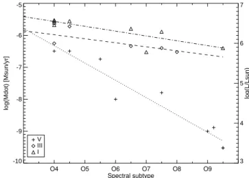
O4 O5 O6 O7 O8 O9 Spectral subtype -10 -9 -8 -7 -6 -5 log(Mdot) [Msun/yr] 3 4 5 6 7 log(L/Lsun) I III V
Fig. 3.Empirically derived mass-loss rates as a function of the spectral
type for O stars of luminosity classes I, III, and V (see legend). Lines show linear fits for each luminosity class. The mass-loss rates of giants and supergiants are uncertain within a factor of 2–3, i.e.,∆ log ˙M ≈ 0.3 − 0.5.
To our knowledge, only a few Galactic O-type giants have been analyzed by advanced clumped stellar atmosphere models (Martins et al. 2005b;Shenar et al. 2015). On the other hand, a significant number of O-type giants were included in the study of Repolust et al.(2004), who measured mass-loss rates using optical spectra and presented the results without correcting for clumping effects. As they note, these values tend to overpredict the real mass-loss rates. To correct the mass-loss rates in giant stars, we note that Oskinova et al. (2007) have shown that the emission in Hα line is not affected by macroclumping even in the dense winds of O supergiants, and therefore can be used as a good mass-loss rate indicator. However, the derived mass-loss rates still have to be corrected because of optically thin clump-ing. Adopting a conservative value of 0.1 for the volume filling factor, the O-giant mass-loss rates fromRepolust et al. (2004) are reduced by a factor of three. The resulting mass-loss rates are given in Table2and Fig.3.
To illustrate the uncertainties associated with the mass-loss measurements and justify our approach, it is useful to con-sider an example: the star HD 93250 is classified as O3V((f)) in Repolust et al.(2004), who obtained its mass-loss rate log ˙M = −5.46+0.11−0.16. Assuming a filling factor of 0.1, the mass-loss rate should be reduced to log ˙M= −5.9.Martins et al.(2005b) clas-sify HD 93250 as O3.5V((f+)). Using clumped models with a filling factor of 0.01, they measure its mass-loss rate as log ˙M= −6.25 ± 0.7. On the other hand, the theoretical mass-loss rate for this star is an order of magnitude higher, log ˙MVink= −5.25. In GOSS, the star is re-classified as O4III. Correspondingly, the theoretical mass-loss rate is log ˙MVink = −5.42. This example illustrates the large discrepancy between theoretical and empiric mass-loss rates, but it shows that the empirical measurements agree within a factor of two to three when clumping is taken into account. This example also illustrates that the errors are largely dominated by the systematic differences between the models. Furthermore, each atmosphere model has errors on mass-loss rates that are due to the errors on the fundamen-tal stellar parameters, distance, and the adopted description of clumping.
The mass-loss rates of O-type dwarfs are much less certain compared to giants and supergiants. Still, the empirically derived mass-loss rates of low-luminosity O dwarfs are orders of
mag-nitude lower than predicted by theoretical recipes. This problem is often referred to as “the weak wind problem” (Martins et al. 2005b). It is interesting to note that nearly all solutions sug-gested to resolve the weak-wind problem in O stars invoke X-rays (Huenemoerder et al. 2012, and references therein). The empirically measured mass-loss rates of well-studied Galactic O-dwarfs are given in Table2. The strong dependence of their mass-loss rate on the spectral type is clearly seen in Fig.3which shows empiric mass-loss rates as a function of spectral type for each luminosity class. It is interesting to note that the depen-dence of mass-loss rate on spectral subtype is much more pro-nounced in dwarf stars than in supergiants.
We performed a linear fit to the recent empiric ˙Mestimates (as described above) and obtained the following scaling rela-tions,
log( ˙M[M yr−1])= −4.2 − 0.5 × SpT for OV stars, (1) log( ˙M[M yr−1])= −5.5 − 0.1 × SpT for OIII stars, (2) log( ˙M[M yr−1])= −5.0 − 0.2 × SpT for OI stars, (3) where “SpT” denotes a corresponding numeric value of a spec-tral subtype; for example, for an O4I star, the value of SpT is 4. Keeping in mind the significant uncertainties in mass-loss measurements, these empiric relations were used to assign the mass-loss rates to the O stars in this study.
4. X-ray parameters
4.1. X-ray fluxes
The 3XMM-DR7 catalog provides count rates in the 0.2–12 keV energy band for each source. To calculate X-ray fluxes on this basis, one needs to establish the energy count rate to flux conver-sion factor (ECF). For this purpose we used the Portable, Inter-active Multi-Mission Simulator (PIMMS). The intrinsic X-ray spectrum emitted by an O-type star was approximated by a col-lisional plasma model, apec (Smith et al. 2001), with solar abun-dances and single temperature kT = 0.35 keV, which is typical for single X-ray emitting O stars (Nazé et al. 2011). For each source in our sample, we calculated unabsorbed X-ray fluxes from the mean PN count rate of all detections. The upper and lower values for the X-ray fluxes based on the mean errors of the count rates were used to estimate the errors of the fluxes. The fluxes were corrected for interstellar absorption using the NH values calculated in Sect.3.2. All the X-ray observations were carried out with medium or thick filters meaning that opti-cal loading should not be an issue. Nevertheless, as a san-ity check, we investigated the summary source detection flag SC_SUM_FLAG and confirmed that no sources in our catalog were flagged for suspected optical loading. As a following step, X-ray luminosities were computed for the distances calculated as described in Sect. 3.3. All stars in our sample have X-ray luminosities in the range 1031−34erg s−1, for either spectropho-tometric or parallactic distance estimates.
Among our sample stars, 60 objects have been observed by XMM-Newton only once. The rest of the sources have been observed and detected 3–4 times on average, and up to 11 times, with individual exposure times ranging from 3 to 100 ks. The unabsorbed fluxes were calculated using the average value of the count rates among all detections for each source. Therefore the fluxes and luminosities presented in this catalog characterize steady X-ray emission of O stars.
O-type stars show typical X-ray variability on the level of ∼10% (e.g.,Oskinova et al. 2001;Nazé et al. 2013;Massa et al. 2014). Time series were automatically extracted by the XMM-Newtonpipeline for 108 out of the 132 O stars we study here. Seven of the stars are classified in the 3XMM-DR7 catalog as variable based on a χ2 variability test: θ1Ori C, HD 193322A, HD 152218, σ Ori AB, HD 97434, ζ Pup, and HD 93129A. An analysis of their X-ray variability is beyond the scope of this paper.
Besides count rates, the 3XMM-DR7 catalog also provides X-ray fluxes for all objects. Comparing them with the fluxes we derived for our sample stars, we find a mean difference in the flux ratio between the XMM-Newton catalog and our derived val-ues of ≈ 1.65. This difference is due to 1) the different adopted X-ray spectral models; the 3XMM-DR7 fluxes are calculated under assumption of a power-law type X-ray spectrum, while we use a thermal plasma model; and 2) the more accurate interstel-lar neutral hydrogen densities towards O stars which we derive in this study.
To place an upper limit on the X-ray luminosity of an O-star which was observed but not detected by XMM-Newton, we built the cumulative distribution function of X-ray fluxes of all sources detected within the same field of view as listed in 3XMM-DR7 catalog. The upper flux limit to a non-detected O star could then be calculated as the flux correction factor 1.65 multiplied by the flux at which 90% of other field sources are detected.
We searched for non-detections and placed upper limits on their X-ray flux. Firstly we searched for O stars within 90000of the center of any XMM-Newton observation, that is, within the field of view. We ensured that the optical positions were within X-ray images, that is, not falling into gaps or outside of X-ray image boundaries (especially for observations performed not in the full window model). Nine O-type stars were observed but are not detected by XMM-Newton.
O stars not detected in X-rays have late spectral subtype in the range O6–O9.5, cover all luminosity classes and have upper X-ray to bolometric flux ratio close to −7. Since the number of non-detected stars is small, we do not expect the distribution of log(LX/Lbol) (see Sect.4.2) to be biased towards high X-ray to bolometric flux ratio.
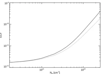
The choice of the plasma temperature and NH affects the calculation of the ECFs and, consequently, the estimated X-ray fluxes. To investigate how robust our derived X-ray luminosities are, we calculated the ECFs for two different plasma tempera-tures, kT = 0.35 keV and kT = 0.5 keV, and for a wide range of NHvalues. As illustrated in Fig.4, a different choice of the plasma temperature in a plausible range leads to an only slightly different ECF. On the other hand, the ECF’s dependence on the NHincreases for larger NHvalues. The average NHof our sample stars is 7 × 1021cm−2(see Fig.1). As can be seen from Fig.4, changing this value by a factor 1.5 results in variation of the ECF by a factor of two. Hence, the ca lculated X-ray fluxes depend mainly on the adopted values of NH.
There are 34 stars in common between ours andNazé(2009) catalogs. The fluxes we obtained for these stars are a factor of two higher, chiefly because we adopted a different relation between EB−Vand NHin our study.
4.2. Correlation between X-ray and bolometric luminosity of O-type stars
Considering the relation between X-ray and bolometric fluxes, log( fX/ fbol), allows us to ignore the problems associated
1021 1022 NH [cm -2] 10-12 10-11 10-10 10-9 ECF
Fig. 4.ECF calculated assuming an APEC model with solar abundance
and temperature of 0.35 keV (solid line) and for 0.5 keV (dotted line) as a function of NH.
with the uncertainties in distances. The bolometric fluxes are calculated according to spectral types of our sample stars as
log( fbol)= −4.6 − (V − AV+ BCV)/2.5. (4)
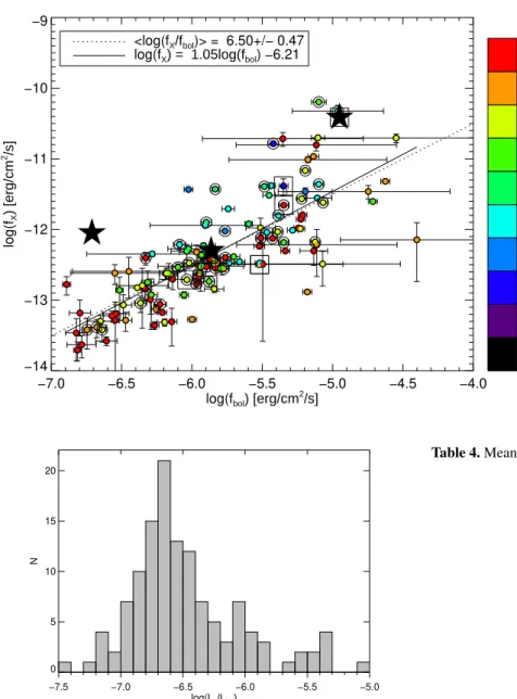
Figure5displays the log( fX/ fbol) relation for the full sam-ple, independent on their luminosity class. Confirming previous studies, we find that the X-ray fluxes scale with the bolometric fluxes. The linear regression fit yields the correlation
log( fX)= −6.21 + 1.05 × log( fbol). (5)
This result is obtained for the total energy band of the XMM-NewtonPN camera (0.2–12 keV). For completeness we include in Appendix Aa similar analysis carried out for two different energy bands (a soft and a hard one).
The bolometric luminosities, Lbol, were derived in two ways. The distance-independent bolometric luminosities are based on spectral type (Martins et al. 2005a). The distance-dependent luminosities (Lbol = 4πd2fbol) are based on bolometric fluxes as obtained using Eq. (5) and Gaia DR2 distances (these luminosi-ties are included in Table1). There is good agreement between bolometric luminosities derived by different methods. We use the distance dependent luminosity since it eliminates distance dependence in log(LX/Lbol).
Figure 6 shows the log(LX/Lbol) distribution for all our sample stars. The log(LX/Lbol) distribution is non-Gaussian, with a peak at around −6.7 and minimum and maximum val-ues at around −7.5 and −5.0 respectively, corroborating previ-ous results based on ROSAT data (Berghoefer et al. 1997). The impact of errors is discussed in AppendixB. As can be seen from Fig.6 the distribution shows a tail towards high values. Bina-rity could result in an increased X-ray flux, for example, due to wind-wind collisions. In the following sections we discuss the dependence of log(LX/Lbol) on luminosity class, spectral type, and binarity.
Although the log(LX/Lbol) distribution is non-Gaussian, we computed average values for log( fX/ fbol) for all stars as a func-tion of the spectral type, for single and binary stars and for two different ranges of spectral types. The results are presented in Table4.
4.2.1. The dependence of log(LX/Lbol) on luminosity class
The log( fX/ fbol) relation for different luminosity classes is shown in Fig.7. The correlation coefficients between X-ray and bolometric fluxes and the 1−σ confidence intervals of the coef-ficients of the linear fits are given in Table3. To measure the strength of the linear correlation, we calculated the Pearson cor-relation coefficient R. This coefficient can take values between 1 and −1. Values close to 1 or −1 reflect a strong positive or neg-ative linear correlation between the two variables, while values close to 0 indicate no relationship.
Dwarfs and giant O stars show a very strong correlation between log( fX) and log( fbol). The O6 IV star ALS 15108 has unusually high log( fX) and log( fbol). We investigated this star in more detail, and found that it has a very high reddening (EB−V ∼ 3.1). The star belongs to the Cygnus OB2 association. The extinction is known to be large in the area. It is likely that we overestimate the neutral hydrogen column density towards this star, leading to its unusually high X-ray luminosity.
The correlation between the X-ray and the bolometric for O supergiants is only moderate4. Despite the relatively small num-ber of O-supergiants in our study, one can see that confirmed spectroscopic binary supergiants have approximately constant bolometric flux (log( fbol) ∼ −5.5), while their X-ray fluxes span over three orders of magnitude (Fig.7).
The log(LX/Lbol) distribution depends on the luminosity class, as illustrated in Fig.8. For dwarf and giant stars the dis-tribution peaks at around −6.6, shifting towards smaller values, −6.8, for supergiant stars. Mean values are −6.6±0.4, −6.5±0.4, and −6.4±0.6 for dwarf, giant, and supergiant stars, respectively. Interestingly, all these averages are above the canonical value of −7. It is important to keep in mind that the log(LX/Lbol) distri-bution is non-Gaussian.
To study the dependence of the log(LX/Lbol) distribution on spectral type, we divided our sample into two groups – early O stars with spectral subtypes in the range O2–O6, and late O stars with spectral subtypes from O6 to O9.5. The log(LX/Lbol) distribution peaks around −6.4 for early O-type stars, and shifts towards lower values close to −6.6 for later spectral types. The mean values are −6.3 ± 0.5 and −6.6 ± 0.4 for early and late spectral types, respectively.
4.2.2. log(LX/Lbol) dependence on binarity
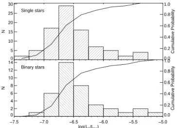
The distribution of log(LX/Lbol) for confirmed binaries is very similar to that of single stars (see Fig.10). Both distributions peak at log(LX/Lbol) ∼ −6.6 and the mean values are −6.6 ± 0.5 and −6.4 ± 0.5 for single and binary stars, respectively. This cor-roborates the results of previous studies (Sciortino et al. 1990; Oskinova 2005; Nazé 2009). Most likely, the true fraction of binaries in our sample is significantly higher than those of the already confirmed binaries, and the list of punitively single stars is very likely contaminated by binaries. A thorough analysis of the confirmed single star sample and confirmed colliding wind binaries is beyond the scope of this paper.
4.3. X-ray hardness-ratios
Among other parameters, the 3XMM-DR7 catalog provides hardness ratios (HR) describing the difference in count rates 4 Interestingly, the weak or absent correlation between X-ray and bolo-metric luminosity was previously noticed in another class of massive stars with dense and fast winds, namely Wolf-Rayet stars (Ignace et al.
−7.0 −6.5 −6.0 −5.5 −5.0 −4.5 −4.0 log(fbol) [erg/cm
2 /s] −14 −13 −12 −11 −10 −9 log(f X ) [erg/cm 2 /s] <log(fX/fbol)> = 6.50+/− 0.47
log(fX) = 1.05log(fbol) −6.21
0
1
2
3
4
5
6
7
8
9
Fig. 5. X-ray flux vs. bolometric flux for O
stars of all luminosity classes and as a function of the spectral subtype (color-coded with ear-lier subtypes being bluer, and the later subtypes being redder). Known spectroscopic binaries are highlighted with a ring around the solid cir-cle, magnetic O stars are represented by aster-isks, and stars flagged as variable are shown with a squared symbol. The linear fit log( fX)= a+ b × log( fbol) and the mean log( fX/ fbol) value are shown as solid and dotted lines, respectively (see text for details).
−7.5 −7.0 −6.5 −6.0 −5.5 −5.0 log(LX/Lbol) 0 5 10 15 20 N
Fig. 6.Distribution of the X-ray to bolometric luminosity ratio for all
the stars in the sample.
Table 3. Number of O stars, correlation coefficient R (see text for its definition), and fit coefficients for log( fX) = a + b × log( fbol).
Lum. Class # R a b All 127 0.78 −6.21 ± 0.44 1.05 ± 0.08 V 60 0.80 −7.05 ± 0.54 0.92 ± 0.09 IV 14 0.83 −7.92 ± 0.94 0.78 ± 0.16 V+IV 74 0.80 −7.15 ± 0.47 0.90 ± 0.08 III 21 0.89 −3.91 ± 1.03 1.45 ± 0.18 I+II 30 0.55 −6.19 ± 1.63 1.04 ± 0.30
between two consecutive bands, defined as HR= count_ratei+1− count_ratei
count_ratei+ count_ratei+1
· (6)
In other words, the HR gives a rough idea of the slope of the X-ray spectrum; for example, HR= 0 would be a flat spectrum, HR > 0 implies the source emits more photons in the harder band, and HR < 0 tells us the source emits more photons in the
Table 4. Mean log( fX/ fbol).
Lum. Class log( fX/ fbol)
All −6.50 ± 0.47 V −6.56 ± 0.39 IV −6.61 ± 0.25 V+IV −6.57 ± 0.37 III −6.51 ± 0.42 I+II −6.40 ± 0.62 SpT early −6.23 ± 0.44 SpT late −6.62 ± 0.43 Single −6.54 ± 0.47 Binaries −6.41 ± 0.46
softer band. The HR value 1 or −1 in 3XMM-DR7 means the source was not detected in either band.
We calculate the mean PN hardness ratios HR2 and HR3 that describe emission in the energy bands 2 and 3, and 3 and 4, and cover the energy ranges 0.5–1.0, 1.0–2.0, and 2.0–4.5 keV, respectively.
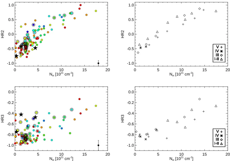
Figure11shows the relation between HRs and NHlimited to sources with errors on HRs lower than 0.3. One can see that, as expected, HR2 increases with NH. There are only a few sources with high HR2 and HR3 at a relatively low NH, these are intrin-sically hard X-ray sources. We computed mean HR in bins of similar NHfor different luminosity classes, and found that super-giant stars have higher HRs at the same NH, as can be seen in particular in the HR2 (right upper panel of Fig.11) but also in the HR3. This shows that supergiant stars have systematically harder spectra than dwarfs.
5. Correlations between X-ray and wind parameters
In this section we investigate the correlations between X-ray luminosity and stellar wind parameters for different spec-tral types and luminosity classes. As explained in detail in Sect.3.4, the stellar wind velocities were measured from the UV
−8 −7 −6 −5 −4 −3 log(fbol) [erg/cm
2/s] −14 −13 −12 −11 −10 −9 log(f X ) [erg/cm 2/s] <log(fX/fbol)> = −6.57 <log(fX/fbol)> = −6.57
log(fX) = 0.90log(fbol) −7.15
log(fX) = 0.90log(fbol) −7.15
V, IV
−8 −7 −6 −5 −4 −3
log(fbol) [erg/cm
2/s] −14 −13 −12 −11 −10 −9 log(f X ) [erg/cm 2/s] <log(fX/fbol)> = −6.51 <log(fX/fbol)> = −6.51
log(fX) = 1.45log(fbol) −3.91
log(fX) = 1.45log(fbol) −3.91
III
−8 −7 −6 −5 −4 −3
log(fbol) [erg/cm
2/s] −14 −13 −12 −11 −10 −9 log(f X ) [erg/cm 2 /s] <log(fX/fbol)> = −6.40 <log(fX/fbol)> = −6.40
log(fX) = 1.04log(fbol) −6.19
log(fX) = 1.04log(fbol) −6.19
I, II
37.5 38.0 38.5 39.0 39.5 40.0 40.5 41.0
log(Lbol) [erg/s]
30 31 32 33 34 35 36 log(L X ) [erg/s] <log(LX/Lbol)> = -6.57 <log(LX/Lbol)> = -6.57
log(LX/Lsun) = 0.95log(Lbol/Lsun) -6.31
log(LX/Lsun) = 0.95log(Lbol/Lsun) -6.31
V, IV
37.5 38.0 38.5 39.0 39.5 40.0 40.5 41.0
log(Lbol) [erg/s]
30 32 34 36 log(L X ) [erg/s] <log(LX/Lbol)> = -6.51 <log(LX/Lbol)> = -6.51
log(LX/Lsun) = 1.42log(Lbol/Lsun) -8.78
log(LX/Lsun) = 1.42log(Lbol/Lsun) -8.78
III
37.5 38.0 38.5 39.0 39.5 40.0 40.5 41.0
log(Lbol) [erg/s]
30 32 34 36 log(L X ) [erg/s] <log(LX/Lbol)> = -6.40 <log(LX/Lbol)> = -6.40
log(LX/Lsun) = 1.33log(Lbol/Lsun) -8.25
log(LX/Lsun) = 1.33log(Lbol/Lsun) -8.25
I, II
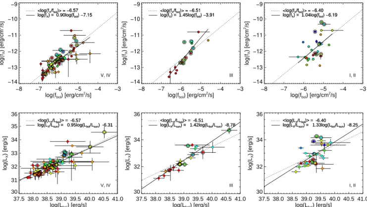
Fig. 7.log( fX/ fbol) (top row) and log(LX/Lbol) (bottom row) relation for O stars of different luminosity classes (V, III, and I from left to right
panels). Known spectroscopic binaries are highlighted with a ring around the solid circle, and spectral types are color coded as in Fig.5. The linear fits log( fX)= a + b × log( fbol) and the mean log( fX/ fbol) values for each case are shown as solid and dotted lines, respectively (see text for details). For O supergiants, the correlations are weak, while they are significant for O dwarf and giant stars (see Table3).
0 5 10 15 20 25 N 0.0 0.2 0.4 0.6 0.8 1.0 Cumulative Probability V, IV 0 2 4 6 N 0.0 0.2 0.4 0.6 0.8 1.0 Cumulative Probability III −7.5 −7.0 −6.5 −6.0 −5.5 −5.0 log(LX/Lbol) 0 1 2 3 4 5 6 N 0.0 0.2 0.4 0.6 0.8 1.0 Cumulative Probability I, II
Fig. 8. log(LX/Lbol) histogram and cumulative distribution function
for dwarfs (top panel), giants (middle panel), and supergiants (bottom panel).
spectra only for 35 stars in our sample. The wind velocities show a general trend of decreasing for later spectral types (see Fig.2), however with a significant scatter. The scatter is also obvious in Fig. 3 which shows the dependence of mass-loss rates on
0 2 4 6 8 10 12 14 N 0.0 0.2 0.4 0.6 0.8 1.0 Cumulative Probability SpT <=6 −7.5 −7.0 −6.5 −6.0 −5.5 −5.0 log(LX/Lbol) 0 10 20 30 N 0.0 0.2 0.4 0.6 0.8 1.0 Cumulative Probability SpT >6
Fig. 9.log(LX/Lbol) histogram and cumulative distribution function for
early O2–O6 subtypes (top panel) and late O6–O9.5 subtypes (bottom panel).
spectral subtype for stars of different luminosity classes. The uncertainty on empirically derived mass-loss rates is about a fac-tor of three. The errors on wind velocities and mass-loss rates propagate to other wind parameters, such as wind kinetic energy and momentum.
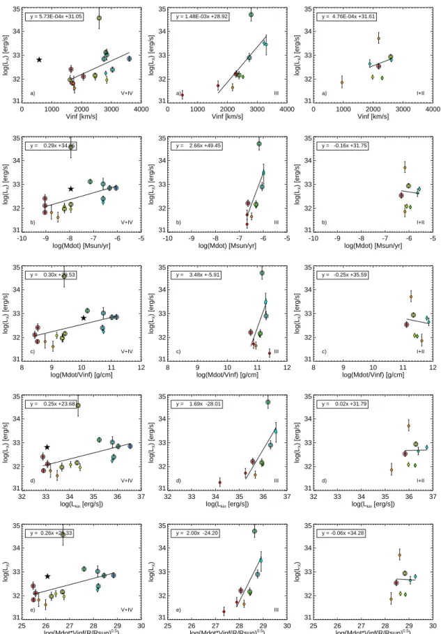
In Fig.12the correlation between X-ray luminosity and wind parameters is shown. To reduce the errors, only the stars with wind velocities empirically measured from the UV spectra are included in this figure. Hence the upper row in Fig.12displays only the measured quantities of the X-ray luminosities and wind velocities for a sub-sample of O stars.
0 5 10 15 20 25 30 N 0.0 0.2 0.4 0.6 0.8 1.0 Cumulative Probability Single stars −7.5 −7.0 −6.5 −6.0 −5.5 −5.0 log(LX/Lbol) 0 2 4 6 8 10 12 14 N 0.0 0.2 0.4 0.6 0.8 1.0 Cumulative Probability Binary stars
Fig. 10.log(LX/Lbol) histogram and cumulative distribution function for
putative single stars (top panel), and in binaries (bottom panel).
The linear fits were performed without taking into account the magnetic stars, and also omitting HD 93521, given its unusually slow wind. We note that there are three other pecu-liar systems with rather low LX and low stellar wind density: HD 14633 (ON8.5V), BN Gem (O8:V, the lowest X-ray lumi-nosity among the whole sample stars), and HD 15137 (O9.5II-III). Results of the linear fits are given in Table 5; the errors in the coefficients correspond to the 1-σ confidence interval.
The correlation between X-ray luminosity and wind velocity is seen for dwarf and giant stars, but is absent for supergiants. As can be seen in Fig.12, for dwarf and giant stars the X-ray lumi-nosities increase as winds increase in speed. Despite relatively large scatter (in particular for dwarfs) which is largely induced by binaries with their higher X-ray luminosities, the overall cor-relation is weak for dwarfs and strong for giant stars. For single stars this correlation implies that stars with later spectral types, that is, stars with lower effective temperatures and lower 3∞, have lower X-ray luminosities. The situation is different for super-giants, where only very weak or no correlation between X-ray luminosity and terminal velocity is found. This may reflect the reality or be simply due to the small number of supergiants with measured 3∞.
Since the wind velocities and X-ray luminosities are empiric measurements, the detected correlations (or their absence) are physical and not induced by systematic errors. This gives us confidence to search for correlations between X-ray luminosi-ties and other wind parameters.
Since spectral types are known for all stars in our sample we can estimate their mass-loss rates using the SpT– ˙M scaling relations Eqs. (1)–(3) derived in Sect.3.4. As can be seen from Fig.12and Table5, the X-ray luminosities show weak correla-tion with mass-loss rate for main sequence and giant stars, while there is basically no correlation for supergiants.
The correlation is also present when considering spectral types within each luminosity class – later spectral subtypes tend to have lower mass-loss rates and lower X-ray luminosities than early spectral subtypes.
As a next step we investigate the scaling of X-ray luminosity with global parameters describing stellar winds, such as the wind kinetic luminosity Lkin= 12M ×3∞˙
2[erg s−1], the density estima-tor Nl =
˙ M 3∞ [g cm
−1], and the modified stellar wind momentum,
D = ˙M × 3∞ × qR∗
R , defined according to Kudritzki & Puls
(2000). Reflecting the scaling of X-ray luminosity with mass-loss rate and wind velocity, the giant O stars show strong correlations with wind parameters, while dwarfs show only weak correlations and no correlation is seen in O supergiants.
The X-ray luminosity of late O-type dwarfs (exhibiting the weak wind problem; see Sect.3.4) is a few percent of the stellar wind kinetic luminosity (see Fig.12). This fraction drops for ear-lier spectral subtypes and for giants and supergiants; for exam-ple, in the latter case LX < 10−3Lkin. The trend showing larger X-ray output from O stars with weaker winds has already been reported (e.g.,Oskinova et al. 2006).
The density parameter Nlis a proxy for the mean wind den-sity, and determines the shock cooling length (see Eq. (14) and its discussion inHillier et al. 1993).Owocki et al.(2013) noticed that for radiative shocks one can expect that LX ∝ ( ˙M/3∞)1−m. Using the theoretically expected scaling between mass-loss rates and bolometric luminosities, they suggested that if the expo-nent m ≈ 0.4 the observed scaling between LXand Lbol can be reproduced.
We test this suggestion using our empiric approach. As can be seen from Fig.12and Table5, for the total ensemble of O stars, the correlation between log(LX) and log Nlis very weak. Only giants show a significant correlation which is different from the one expected theoretically.
Considering the modified wind momentum, we notice simi-lar trends as for other wind parameters – a significant correlation is observed for dwarfs and giants, while no correlation is seen for supergiant stars in Fig.12. The analysis byMokiem et al.(2007) confirmed theoretical expectations that modified wind momenta do not depend on stellar luminosity class (when not account-ing for the weak wind star problem). In this study we choose the empiric approach, and for low-luminosity dwarfs we adopt empiric mass-loss rates which are significantly lower that those predicted theoretically. Figure12shows that the scaling relations between X-ray luminosity and wind parameters are quite di ffer-ent for different luminosity classes.
To measure the strength of the correlation between X-ray luminosity and wind parameters we calculated the Pearson cor-relation coefficients. We also used a non-parametric method, in particular we calculated the Spearman’s rank correlation coef-ficient ρ. The Spearman coefficient can take values between 1 and −1. Values close to 1 or –1 reflect a strong positive or negative monotonic correlation (not necessarily a linear corre-lation such as for the Pearson coefficient) between the two vari-ables, while values close to 0 indicate no relationship. Results are listed in Table5. Values obtained for R and ρ suggest that the X-ray luminosity of supergiant stars is not correlated with wind parameters. We provide linear fits between X-ray luminos-ity and wind parameters for each luminosluminos-ity class in Table5. For supergiant stars, fitting the X-ray luminosity to a constant gives log(LX)= 32.68 ± 0.21.
This raises the key question on the origin of the LX–Lbol cor-rection for O-stars – is the X-ray luminosity determined by fun-damental stellar parameters or by wind strength? – a problem analogous to the question “which came first, the chicken or the egg?”. In the former case, X-rays could be associated with small-scale magnetic fields on the stellar photosphere (Oskinova et al. 2011, and references therein), which in turn depend on sub-surface structure (Cantiello & Braithwaite 2011; Urpin 2017). The latter case is the well accepted scenario of X-ray generation by strong shocks in stellar winds resulting from the line driven instability (Feldmeier et al. 1997).
0 5 10 15 20 NH [10 21 cm-2] -1.0 -0.5 0.0 0.5 1.0 HR2 0 5 10 15 20 NH [10 21 cm-2] -1.0 -0.5 0.0 0.5 1.0 HR2 I-II III IV V I-II III IV V I-II III IV V I-II III IV V I-II III IV V I-II III IV V I-II III IV V I-II III IV V I-II III IV V I-II III IV V I-II III IV V I-II III IV V I-II III IV V I-II III IV V 0 5 10 15 20 NH [10 21 cm-2 ] -1.0 -0.8 -0.6 -0.4 -0.2 0.0 HR3 0 5 10 15 20 NH [10 21 cm-2 ] -1.0 -0.8 -0.6 -0.4 -0.2 0.0 HR3 I-II III IV V I-II III IV V I-II III IV V I-II III IV V I-II III IV V I-II III IV V I-II III IV V I-II III IV V I-II III IV V I-II III IV V I-II III IV V I-II III IV V I-II III IV V I-II III IV V
Fig. 11.Hardness ratios HR2 (top panels) and HR3 (bottom panels) as a function of NH. In the left panels symbols have been colored according to
the spectral type as in Fig.5and mean error in the HR is indicated in the lower right corner of the plot. In the right panels, mean HRs have been calculated per bin of NHand different luminosity classes; different symbols stand for different luminosity classes as indicated in the legend.
As mentioned earlier, these results are based on a lim-ited sample of 35 stars with measured stellar wind veloci-ties. Although these wind velocities are decreasing towards later spectral subtypes, there is a significant scatter at each spectral subtype, a scatter also present in the dependence of mass-loss rates on spectral subtype for stars of different lumi-nosity classes. Errors on wind velocities and mass-loss rates propagate to other wind parameters, such as wind kinetic energy and momentum. A larger sample of stars with measured wind velocities and mass-loss rates would help to better constrain the correlations between X-ray luminosity and stellar wind parameters.
For completeness, in AppendixCwe show the correlations between bolometric luminosity and stellar wind parameters.
6. Summary and conclusions
The spectroscopic sample of Galactic O stars, GOSS (Sota et al. 2014;Maíz Apellániz et al. 2016), was used to investigate, in a homogeneous and consistent way, the X-ray emission from O stars. We found that 127 stars from GOSS have an unambigu-ous counterpart in the 3XMM-DR7 catalog of X-ray sources and are associated to a Gaia-DR2 source. The stellar param-eters of O stars were obtained using spectral calibrations pre-sented byMartins et al. (2005a). Mass-loss rates of O stars of different spectral types and luminosity classes were compiled
from the literature and used to derive an empirical spectral-type mass-loss rate relation. From this empirical relation we derived mass-loss rates for all our sample stars. Terminal velocities from Prinja et al.(1990) are available for a subsample of 35 of these stars. For this subsample of O stars, wind parameters (kinetic luminosity, momentum and density) were estimated based on the empirically derived mass-loss rates and the measured terminal velocities.
Interstellar extinction was estimated on the basis of optical photometry available for all our sample stars. The stellar dis-tances were estimated on the basis of stellar photometry as well using Gaia DR2. The X-ray hardness ratios and fluxes were cal-culated from count rates provided in the 3XMM-DR7 catalog, while X-ray luminosities are based on dereddened fluxes and GaiaDR2 parallactic distances.
We confirm that X-ray luminosities of dwarf and giant O stars correlate with their bolometric luminosities. For the sub-sample of O dwarf and giant stars with known terminal veloci-ties we find that their X-ray luminosiveloci-ties are correlated with their key wind parameters, such as terminal velocity, mass-loss rate, wind kinetic energy, and wind momentum. However, these cor-relations break down for supergiant stars. Furthermore, O super-giants have systematically harder X-ray spectra than dwarf and giant stars at any given interstellar extinction. We show that the distribution of log(LX/Lbol) in our sample is non-Gaussian, with the peak of the distribution at log(LX/Lbol) ≈ −6.6, minimum value log(LX/Lbol) ≈ −7.5, and a longer tail towards higher
0 1000 2000 3000 4000 Vinf [km/s] 31 32 33 34 35 log(L X ) [erg/s] y = 5.73E-04x +31.05 V+IV a) 0 1000 2000 3000 4000 Vinf [km/s] 31 32 33 34 35 log(L X ) [erg/s] y = 1.48E-03x +28.92 III a) 0 1000 2000 3000 4000 Vinf [km/s] 31 32 33 34 35 log(L X ) [erg/s] y = 4.76E-04x +31.61 I+II a) -10 -9 -8 -7 -6 -5 log(Mdot) [Msun/yr] 31 32 33 34 35 log(L X ) [erg/s] y = 0.29x +34.65 V+IV b) -10 -9 -8 -7 -6 -5 log(Mdot) [Msun/yr] 31 32 33 34 35 log(L X ) [erg/s] y = 2.66x +49.45 III b) -10 -9 -8 -7 -6 -5 log(Mdot) [Msun/yr] 31 32 33 34 35 log(L X ) [erg/s] y = -0.16x +31.75 I+II b) 8 9 10 11 12 log(Mdot/Vinf) [g/cm] 31 32 33 34 35 log(L X ) [erg/s] y = 0.30x +29.53 V+IV c) 8 9 10 11 12 log(Mdot/Vinf) [g/cm] 31 32 33 34 35 log(L X ) [erg/s] y = 3.48x +-5.91 III c) 8 9 10 11 12 log(Mdot/Vinf) [g/cm] 31 32 33 34 35 log(L X ) [erg/s] y = -0.25x +35.59 I+II c) 32 33 34 35 36 37 log(Lkin [erg/s])
31 32 33 34 35 log(L X ) [erg/s] y = 0.25x +23.68 V+IV d) 32 33 34 35 36 37 log(Lkin [erg/s])
31 32 33 34 35 log(L X ) [erg/s] y = 1.69x -28.01 III d) 32 33 34 35 36 37 log(Lkin [erg/s])
31 32 33 34 35 log(L X ) [erg/s] y = 0.02x +31.79 I+II d) 25 26 27 28 29 30 log(Mdot*Vinf(R/Rsun)0.5) 31 32 33 34 35 log(L X ) y = 0.26x +25.33 V+IV e) 25 26 27 28 29 30 log(Mdot*Vinf(R/Rsun)0.5) 31 32 33 34 35 log(L X ) y = 2.00x -24.20 III e) 25 26 27 28 29 30 log(Mdot*Vinf(R/Rsun)0.5) 31 32 33 34 35 log(L X ) y = -0.06x +34.28
Fig. 12.X-ray luminosity as a function of wind parameters. Only the stars with wind velocities measured from the UV spectra are shown. The
mass-loss rates are uncertain within a factor of 2–3 due to systematic errors, i.e.,∆ log ˙M ≈0.3−0.5 (see Sect.3.4for a discussion on errors). From left to right columns: results for dwarfs, giants, and supergiants. First row from the top: correlations with wind terminal velocity; second row from the top: dependence on mass-loss rate calculated using the empirical SpT– ˙Mrelations derived in Sect.3.4; middle row: dependence on wind density; fourth row from the top: dependence on wind kinetic luminosity; bottom row: dependence of X-ray luminosity on modified stellar wind momentum. The color coding of different spectral subtypes is the same as in Fig.5. Linear fits are shown with a line.