HAL Id: hal-00508680
https://hal.archives-ouvertes.fr/hal-00508680
Submitted on 5 Aug 2010
HAL is a multi-disciplinary open access
archive for the deposit and dissemination of
sci-entific research documents, whether they are
pub-lished or not. The documents may come from
teaching and research institutions in France or
abroad, or from public or private research centers.
L’archive ouverte pluridisciplinaire HAL, est
destinée au dépôt et à la diffusion de documents
scientifiques de niveau recherche, publiés ou non,
émanant des établissements d’enseignement et de
recherche français ou étrangers, des laboratoires
publics ou privés.
A new data-based modelling method for identifying
parsimonious nonlinear rainfall/flow models
Vincent Laurain, Marion Gilson, Sylvain Payraudeau, Caroline Grégoire,
Hugues Garnier
To cite this version:
Vincent Laurain, Marion Gilson, Sylvain Payraudeau, Caroline Grégoire, Hugues Garnier. A new
data-based modelling method for identifying parsimonious nonlinear rainfall/flow models.
Interna-tional Congress on Environmental Modelling and Software, IEMSS 2010, Jul 2010, Ottawa, Canada.
pp.CDROM. �hal-00508680�
Modelling for Environment’s Sake, Fifth Biennial Meeting, Ottawa, Canada David A. Swayne, Wanhong Yang, A. A. Voinov, A. Rizzoli, T. Filatova (Eds.) http://www.iemss.org/iemss2010/index.php?n=Main.Proceedings
A new data-based modelling method for
identifying parsimonious nonlinear rainfall/flow
models
V. Lauraina, M. Gilsona, S. Payraudeaub, C. Gr´egoireband H. Garniera
aCentre de Recherche en Automatique de Nancy (CRAN), Nancy-Universit´e, CNRS, BP 70239, 54506 Vandoeuvre-les-Nancy Cedex, France ([email protected]) bLaboratoire d’Hydrologie et de G´eochimie de Strasbourg ,Universit´e de Strasbourg/ENGEES,
CNRS UMR 7517, 1 quai Koch BP. 61039 F, 67 070 Strasbourg Cedex, France
Abstract: The identification of rainfall/runoff relationship is a challenging issue, mainly because
of the complexity to find a suitable model for a whole given catchment. Conceptual hydrological models fail to describe correctly the dynamic changes of the system for different rainfall events (e.g. intensity or duration). However, the need for such relationship grows with the water pol-lution increase in agricultural regions. Lately, a well-known type of model in the control field appears to be a suitable candidate for water processes identification: the Linear Parameter Vary-ing (LPV) models. This paper depicts a novel refined instrumental variable based method for the identification of Input/Output LPV models and this algorithm is applied to identify a parsimonious nonlinear rainfall/flow model of a 42 ha vineyard catchment located in Alsace, France.
Keywords: data-based modelling, linear parameter varying models, refined instrumental variable,
rainfall, runoff, vineyard
1 INTRODUCTION
This work is inscribed in the data-based mechanistic (DBM) framework which delivers some stochastic solution to the “top-down ” modelling methods at the catchment scale. The aim is to deliver a parsimonious model which avoids the identifiability issues linked with the high number of parameters in conceptual models (Mambretti and Paoletti (1996); Previdi et al. (1999),Young (2003)). Nonetheless, the obtained model can be classified as hybrid metric–conceptual model as it is optimized given some set of measured data, but the model set is defined based on some conceptual assumptions. The far-end goal is to deliver a solution for the simulation of the rain-fall/pollutant relationship at the catchment scale for intelligent environmental decision support. In aiming at solving this challenging problem, a solution for rainfall/runoff modelling is proposed as a preliminary work.
The identification of rainfall/runoff relationship is a challenging issue, mainly because of the com-plexity to find a suitable model for a whole given catchment (Beven (2000)). The need for such relationship grows with the size of drainage networks in urban catchments or with the water pollu-tion increase in agricultural regions. In rural catchments, there is a high spatio-temporal variability of the soil property whether it lies in the vegetation, in the soil type or evapotranspiration (Young and Garnier (2006)) and there is a high difference between the total and efficient rainfall. In this case, linear models most often completely fail in delivering a satisfying rainfall/flow relationship. The use of nonlinear models requires the choice for a nonlinearity. Some nonparametric meth-ods for estimating these nonlinearities such as state dependent parameters (SDP) were introduced (Young and Garnier (2006)). Lately, a well-known type of model in the control field appears to be a suitable candidate for water processes identification (Previdi and Lovera (2009)): the Linear
V. Laurain et al. / A new data-based modelling method for identifying parsimonious nonlinear rainfall/flow models
Parameter Varying (LPV) models. LPV models depend on so-called scheduling variables and a
challenging issue is to define which variables the system depends on.
The main contribution of this paper lies in the use of a recently developed refined instrumen-tal variable (RIV) based method for the identification of Input/Output LPV models with colored ARMA-type added noise for the estimation of the rainfall/runoff relationship in rural catchments. This method produces consistent estimates even when the noise assumption is not fulfilled, which is a strong feature for stochastic optimization based methods. The paper is organized as follows. In Section 2, the main issues for applying data-based identification methods in environmental framework are given. Then, in Section 3, a new LPV identification method based on the refined instrumental variable algorithm introduced in Laurain et al. (2010) is fully detailed. Finally, in Section 4, the full identification process and the model used for rainfall/flow modeling is given while the performance of the presented algorithm are depicted using a data set coming from a 42 ha vineyard catchment located in Alsace, France (Gr´egoire et al. (2010)).
2 ISSUES IN ENVIRONMENTAL DATA-BASED MODELLING
When considering data-based modelling of dynamic systems, most of the optimization methods are based on stochastic optimization methods. Nonetheless, a suited optimization method has to be developed with respect to the field of application considered. In the present context, the fol-lowing features have to be taken into consideration. Most environmental models derive from the first principle of physics. These models are therefore naturally expressed in terms of differential equations which are equivalent to continuous-time transfer functions in the Control community. Therefore, the first issue is the ability to identify a model under its transfer function form which offers the ability to interpret a posteriori the data-based model in physical or ecological terms: data-based mechanistic modelling (Young and Beven (1994)).
The second concern when dealing with environmental data is the inability to control the input and to only be able to measure it. This leads to a so-called Error-In-Variables (EIV) identifi-cation problem. However, the methods developed so far concerning EIV problems need strong hypothesis and knowledge about the noise model (Thil et al. (2009)). In a more general way, speaking about stochastic optimization implies a stochastic representation of the measurement noise. However, the usual gaussian noise assumption is not verified in these rural catchments. When measuring flow, the measurement noise presents complicated characteristics such as non stationarity. For example, the noise variance increases with the flow whereas the variance be-comes null when no flow is measured. During strong rainfall events, some transported particules remain in the channel of the flowmeter, luring him into measuring inexistent flow.
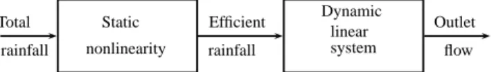
The final challenge concerning rainfall/runoff relationship is to determine the non-linearity of the studied system. The common approximation of conceptual models for rainfall/flow relationship is the Hammerstein structure as presented in Fig 1. In order to estimate such models, the SDP models introduced in Young and Beven (1994) are combined to a fixed interval smoothing filter in order to determine the non-linearity form. This method is very powerful as it is a non-parametric method which does not need the knowledge about the dynamic of the system. The state
depen-Total rainfall Efficient rainfall Outlet flow Static nonlinearity Dynamic linear system
Figure 1: Hammerstein model for rainfall/flow relationship
dant parameter models are similar from a general point of view to LPV models which are widely used in the control theory. These models rely on models in which the parameters depend on a state of the system or a external variable. Nonetheless, the SDP models were mainly restrained so far to Hammerstein structures (Young (2003)) but the relevance of full LPV models for rainfall/flow modeling in urban catchments can be found in Previdi and Lovera (2009). However, until recently (Laurain et al. (2010)), the accurate identification of such models for LPV Output Error (OE) model was not clearly defined in the literature. Therefore, the next section introduces the method from (Laurain et al. (2010)) and the type of model it can be applied to.
3 ESTIMATION OFLPVOUTPUTERRORMODELS
Would the system be linear, a method dealing robustly with the noise conditions depicted in the previous section is the Simplified Refined Instrumental Variable (SRIV) method proposed in Young and Jakeman (1980). Moreover, this method was extended to non-linear models (Laurain et al. (2008)). This section exposes the extension of the SRIV method to LPV-OE models: the LPV-SRIV method. In the LPV case, most of the methods developed for Input/output (IO) mod-els based identification are derived under a linear regression form (Wei and Del Re (2006); Giarr´e et al. (2006); Butcher et al. (2008)). By using the concepts of the Linear Time Invariant (LTI) prediction error framework, recursive least squares (LS) and instrumental variable (IV) methods have been also introduced (Giarr´e et al. (2006); Butcher et al. (2008)). A discussion about the performances and robustness of these algorithms compared to the one introduced in this paper can be found in Laurain et al. (2010).
3.1 LPV output error models
The considered models in this application are given as:
M (
A(pk, q−1)χ(tk) = B(pk, q−1)u(tk−d)
y(tk) = χ(tk) + e(tk)
(1) whered is the delay, χ is the noise-free output, u is the input, e is the additive noise with bounded
spectral density,y is the noisy output of the system and q is the time-shift operator, i.e. q−iu(t k) =
u(tk−i). p are the so-called scheduling variables. For LTI systems, the coefficients of A and B
are constant in time while they are time-varying depending onp for LPV models. A(pk, q−1) and
B(pk, q−1) are polynomials in q−1of degreenaandnbrespectively:
A(pk, q−1) = 1 + na
X
i=1
ai(pk)q−iwith ai(pk) = ai,0+ nα X l=1 ai,lfl(pk) i = 1, . . . , na (2) B(pk, q−1) = nb X j=0 bj(pk)q−iwith bj(pk) = bj,0+ nβ X l=1 bj,lgl(pk) j = 0, . . . , nb. (3)
In this parametrization,{fl}nl=1α and{gl}nl=1β are functions ofp, with static dependence, allowing
the identifiability of the model (pairwise orthogonal functions for example). It can be noticed that the knowledge of{ai,l}ni=1,l=1a,nα and{bj,l}nj=0,l=0b,nβ ensures the knowledge of the full model.
Therefore, these model parameters are stacked columnwise in the parameter vectorρ, ρ=£ a1 . . . an
a b0 . . . bnb
¤⊤
∈ Rnρ, n
ρ= na(nα+ 1) + (nb+ 1)(nβ+ 1)
ai=£ ai,0 ai,1 . . . ai,n
α ¤ ∈ Rnα+1and b j = £ bj,0 bj,1 . . . bj,nβ ¤ ∈ Rnβ+1.
The model defined by equations (1),(2) and (3) is denoted as LPV-OE.
3.2 Identification problem statement
For models given in (1) and assuming that:
• the scheduling variables p are known a priori, • the functions {fl}nl=1α and{gl}nl=1β are known a priori,
• the orders na,nb,nα,nβandd are known a priori,
the identification problem can then be stated as follows: given the total rainfall datau and the
outlet flow datay sampled at times tkk= 1..N , estimate the associated parameter vector ρ. 3.3 Reformulation of the model
A way to solve the LPV identification problem is to rewrite the signal relations of (1) into the following form (Laurain et al. (2010)):
Mρ χ(tk) + na X i=1 ai,0χ(tk−i) | {z } F(q−1)χ(tk) + na X i=1 nα X l=1 ai,lfl(pk)χ(tk−i) | {z } χi,l(tk) = nb X j=0 nβ X l=0 bj,lgl(pk)u(tk−d−j | {z } ) uj,l(tk) y(tk) = χ(tk) + e(tk)
V. Laurain et al. / A new data-based modelling method for identifying parsimonious nonlinear rainfall/flow models
(4) whereF(q−1) = 1 +Pna
i=1ai,0q−i. Note that in this way, the LPV-OE model is rewritten as a Multiple-Input Single-Output (MISO) system with(nb+ 1)(nβ+ 1) + nanαinputs{χi,l}ni=1,l=1a,nα
and{uj,l}nj=0,l=0b,nβ . Given the fact that the polynomial operator commutes in this representation
(F(q−1) does not depend on p
k), (4) can be rewritten as y(tk) = − na X i=1 nα X l=1 ai,l F(q−1)χi,l(tk) + nb X j=0 nβ X l=0 bj,l F(q−1)uj,l(tk) + H(q)e(tk), (5)
which is a LTI representation.
3.4 LPV-SRIV algorithm
In this section a detailed RIV based algorithm is described. The choice for such method can be justified by the facts that in the LTI case, RIV methods lead to statistically optimal estimates if the noise model is correct (S¨oderstr¨om and Stoica (1983)) and provides consistent estimates in case the noise assumption is not fulfilled. This feature is necessary in the present context due to the noise particularity given in Section 2. Any theoretical justification about the LPV-SRIV algorithm can be found in Laurain et al. (2010) but due to space restrictions, only the algorithm is detailed here:
LPV-SRIV algorithm:
Step 1: Use a traditional LS method to obtainρˆ(0)). Set τ = 0.
Step 2: Compute an estimate ofχ(tk) by simulating the auxiliary model:
A(pk, q−1,ρˆ(τ )) ˆχ(tk) = B(pk, q−1,ρˆ(τ ))u(tk−d)
based on the estimated parameters ρˆ(τ ) of the previous iteration. Deduce the output terms
{ ˆχi,l(tk)}ni=1,l=0a,nα as given in (4) using the modelMρˆ(τ ).
Step 3: Compute the estimated filter ˆQ(q−1,ρˆ(τ )) = 1
F(q−1,ρˆ(τ )) and filter the signals
{uj,l(tk)}nj=0,l=0b,nβ , y(tk) and {χi,l(tk)}i=1,l=0na,nα using Q(q−1,ρˆ(τ )) to obtain {uj,lf (tk)}nj=0,l=0b,nβ ,
yf(tk) and {χfi,l(tk)}ni=1,l=0a,nα respectively.
Step 4: Build the filtered estimated regressorϕˆf(tk) and the so called filtered instrument ˆζf(tk)
defined as: ˆ ϕf(tk) =£ −yf(tk−1) . . . −yf(tk−na) − ˆχ f 1,1(tk) . . . − ˆχfna,nα(tk) u f 0,0(tk) . . . ufnb,nβ(tk) ¤⊤ ˆ ζf(tk) =£ −ˆχf(tk−1) . . . − ˆχf(tk−na) − ˆχ f 1,1(tk) . . . − ˆχfna,nα(tk) u f 0,0(tk) . . . ufnb,nβ(tk) ¤⊤
Note that in IV based identification methods, the optimal choice for the instrument is the noise-free version of the regressorϕ(tk) (S¨oderstr¨om and Stoica (1983).
Step 5: The solution of the IV estimation equations can be stated as:
ˆ ρ(τ +1)(N ) = "N X k=1 ˆ ζf(tk) ˆϕ⊤f (tk) #−1 N X k=1 ˆ ζf(tk)yf(tk)
whereρˆ(τ +1)(N ) is the IV estimate of the process model associated parameter vector at iteration τ+ 1 based on the prefiltered input/output data.
Step 6: Ifρ(τ +1)has converged or the maximum number of iterations is reached, then stop, else
increaseτ by1 and go back to Step 2.
4 IDENTIFICATION OF A RAINFALL/RUNOFF RELATIONSHIP IN A RURAL CATCHMENT
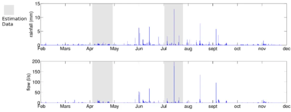
Given the total rainfall datau and the outlet flow data y sampled at times tk,k= 1, . . . , N , the
goal is to estimate the rainfall/runoff relationship. In the given case, the sample time is 6 minutes, the flow unit is l/s and the rainfall is expressed in mm. The data measured during the year 2008 are shown in Fig 2.
Figure 2: Rainfall and flow data for the Hohrain catchment (Alsace, France) during 2008
4.1 Catchment description
The studied Hohrain catchment area is located in the Alsatian vineyard (Eastern part of France, latitude 47579 N; longitude 007173 E; altitude 284 m). The area of the catchment is 42 hectares. Exceptional annual precipitations maximally reached 867 mm (1999) and minimally 361 mm (1953). The average annual rainfall calculated since 1946 is 600 mm. The mean slope of the catchment is 15%. Geologically, W¨urm loamy loess and Oligocene clayey conglomerates and marls, as well as compact calcareous substrate largely dominate in the upper and lower parts of the catchment, respectively. The main soil type is mostly calcareous clay loams with medium infiltration capacity. 68% of the hydraulic catchment are covered by vineyards (Figure 3). The land use shows a gradient from mostly forested areas and partly orchard at the upstream of the basin to agricultural and vineyard areas nearer to the outlet. With more than 120 farming plots, it should be noted that the road network is dense, mostly impervious and represents about 6% of the area of catchment. The catchment can be qualified as dry catchment with no permanent flow (Gr´egoire et al. (2010)). The hydrological functioning can be summarized in three steps: i) first of all no river network is observed and no discharge occurs without rainfall, ii) then, from a total rainfall depth of 4 mm only the road network contributes to the discharge, iii) finally, over a total rainfall depth of 8 mm, the number of fields contributing to the discharge increases with both intensity and total rainfall depth. The catchment is depicted in Fig. 3.
V. Laurain et al. / A new data-based modelling method for identifying parsimonious nonlinear rainfall/flow models
4.2 Preliminary study
Over the70000 samples acquired, only 5000 are greater than 0.3 l/s and are relevant for the
iden-tification process. The dataset has to be split into ideniden-tification data (on which the ideniden-tification algorithm will be run) and validation data. The identification data needs to include the widest possible dynamic range and therefore needs to incorporate both low rainfall events and strong rainfall events. Consequently, the chosen identification data are exposed in Fig. 2 and all the whole dataset is used for the validation of the estimated model. The accuracy of the estimated models is computed using the NASH coefficient defined as (Nash and Stucliffe (1970)):
N ASH= 1 − kˆy(tk) − y(tk)k
var(y(tk))
. (6)
According to section 3.2, a preliminary study is needed in order to determine i)the choice of the scheduling variables, ii) the pure delay of the system and iii) the orders of the system. Trying to optimize all three choices simultaneously is an impossible goal considering all possible combina-tions of scheduling variables. Therefore, the choice of the delay and of the orders will be treated separated from the choice of the scheduling variables.
Order determination: The choice of orders is driven using the assumption that the best LPV
model and the best linear model have the same ordersnbandnaand delayd. This is mainly
mo-tivated by the fact that the linear model is a truncation of a more precise LPV model (fornα= 0
andnβ= 0).
Both the orders and the delay of the model are computed in an automated manner by identifying linear models and minimizing the Young’s Information Criterion (YIC) defined as (Young and Jakeman (1980)):
Y IC= logvar(ˆy(tk) − y(tk))
var(y(tk)) + log 1 nθ nθ X i=1 ˆ πii ˆ ρi (7)
where πii is theith, ithelement of the covariance matrixPρ associated toρ. The method usedˆ
is the LPV-SRIV algorithm wherenα = 0 and nβ = 0 which is equivalent to the SRIV method
(Garnier and Wang (2008)). Minimizing the YIC criterion is equivalent to jointly minimize the
NASH coefficient on the one hand and the order of the system on the other hand. The results
obtained for this catchment arenb= 1, na= 1 and d = 1.
Scheduling variables determination: The final task of the preliminary study is the definition of
the scheduling variables pi(tk). The expert knowledge states that the system behavior changes
with the moisture of the catchment. Nonetheless, such measure is unaccessible in practice and in the presented example, the only accessible data are the total rainfall and the outlet flow. Concern-ing the determination of these schedulConcern-ing variables, most of the work presented here is largely inspired by the recent work of P. Young. In Young (2002), the authors propose a Hammerstein structure (see Fig. 1) where the non-linearity depends on the measured flow in a forecasting con-text: this hypothesis reflects the fair assumption that the outlet flow is well correlated with the moisture of the catchment. More recently ( Young (2003) see and the prior references therein), P. Young proposed a model for simulation in which the nonlinearity depends on output of a lin-ear tank model obtained from the data with some successful interpretation capability. Therefore, based on the same correlation assumption as in Young (2003) and expert knowledge, two schedul-ing variables are proposed to represent as closely as possible the moisture of the field are:
• the outlet flow ˆyL(tk) simulated using a linear model estimated from the data using SRIV
algorithm and(1 + a0q−1)ˆyL(tk) = b0q−1u(tk).
• The sum of the past rainfall ¯u(tk) =P ∆
i=0u(tk−i). ∆ is chosen as the minimum number
of samples maximizing theN ASH coefficient for the LPV model. In this application it is
set to 20 samples or 2 hours.
As a conclusion of this preliminary study, the LPV model considered (LPV-OE) is given by (1) where:
(
A(ˆyL(tk), ¯u(tk), q−1) = 1 +(a1,0+a1,1yˆL(tk)+a1,2u(t¯ k))q−1
B(ˆyL(tk), ¯u(tk), q−1) = (b1,0+ b1,1yˆL(tk) + b1,2u(t¯ k))q−1.
4.3 Results
In this section, the results exposed will focus in showing i) the relevance of the LPV model and ii) the relevance of using a consistent method for unknown noise structure. Therefore, the presented algorithm will be compared to LS based methods which assume Auto Regressive models with
eXogenous inputs (ARX) where the noise has the same dynamic as the system, whether it is a
linear model (ARX),
(1 + a0q−1)y(tk) = b0q−1u(tk) + e(tk), (9)
or a LPV model (LPV-ARX)
A(ˆyL(tk), ¯u(tk), q−1)y(tk) = B(ˆyL(tk), ¯u(tk), q−1)u(tk) + e(tk). (10)
These models are not realistic in practical applications, but they remain widely used because of their simple algorithmic. On the other side, they are so far the only alternative to IV methods when estimating LPV models. The ARX models are estimated using LS methods while the Lin-ear/LPV OE models are estimated using the presented SRIV/LPV-SRIV algorithm. The different
NASH coefficients computed on the validation dataset from the linear ARX and OE1models are
N ASHARX = 0.54 and N ASHOE = 0.63 respectively. Both linear models are unable to
ac-curately fit the data as they cannot model the change of dynamics in the system according to the amount of rain. Nonetheless, the algorithm used for parameter estimation indubitably plays an important role as the model estimated using the SRIV method fits the data much better than the one stemming from the least squares technique.
When estimating the LPV-OE model, using the presented algorithm, the computedN ASH
coef-ficient isN ASHLP V −OE = 0.84. Concerning the LPV-ARX model, the LS method was unable
to provide a stable model and therefore the results are not valid.
Fig. 4(b) and 4(a) show the response of the estimated LPV-OE model and linear OE model for an important rainfall (used for the estimation) and a small rainfall (not used for the estimation) events respectively. It can be seen that the results corroborate the assumption that the chosen scheduling variables represent well the moisture of the catchment.
100 200 300 400 500 0 2 4 6 8 10 12 14 16 18 time (min) flow (l/s) Measured flow Linear Simulation LPV Simulation
(a) Small rainfall event
20 40 60 80 100 120 20 40 60 80 100 120 140 160 180 time (min) flow (l/s) Measured flow Linear Simulation LPV Simulation
(b) Important rainfall event
Figure 4: Comparison of linear and LPV models
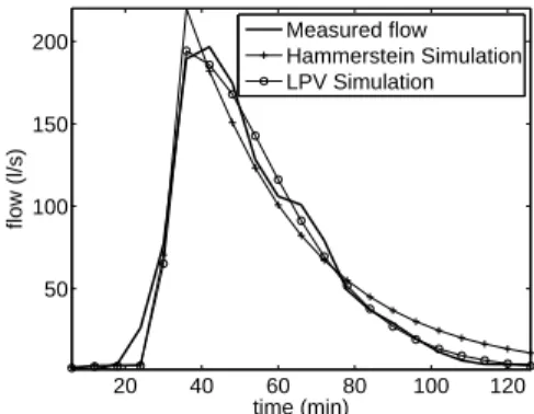
Moreover, the presented model is compared to the nonlinear model proposed in Young (2003) which can be parented to an advanced Hammerstein model. On the validation set, theN ASH
coefficient obtained for this Hammerstein model isN ASHHamm= 0.835. One of the advantage
in using a full LPV model over an Hammerstein structure can be depicted in Fig. 5. The Hammer-stein model only allows changes in the amount of the water reaching the outlet with a fix dynamic constraint while the LPV model allows a large dynamic variation which results in a slightly better fit of the model on this event. Nonetheless, some further investigation is needed to emphasis the physical legitimacy of one or the other model and the only conclusion that can be drawn out is that both models present equivalent statistical performances.
1Linear OE model: y(t
k) = b0q
−1
V. Laurain et al. / A new data-based modelling method for identifying parsimonious nonlinear rainfall/flow models 20 40 60 80 100 120 50 100 150 200 time (min) flow (l/s) Measured flow Hammerstein Simulation LPV Simulation
Figure 5: Comparison between full LPV model and Hammerstein model
5 CONCLUSION
This paper has presented a new algorithm for consistently estimating LPV model when the as-sumed noise model is unknown or false. The theoretical results from (Laurain et al. (2010)) were successfully applied to a dataset from a vineyard catchment. The algorithm based on the refined instrumental variable algorithm outperforms the existing algorithms based on least squares algo-rithm: it leads to consistent estimates under harsh noise conditions. Moreover, some scheduling variables were introduced and their correlation with the moisture of the field has been verified. In order to completely fulfill the data-based mechanistic process, the identification of continuous-time LPV models directly deriving from the first principle laws of physics is intended.
REFERENCES
Beven, K. J. Rainfall-Runoff Modelling: The Primer. John Wiley, Hoboken, NJ, 2000.
Boukhris, A., S. Giuliani, and G. Mourot. Rainfall-runoff multi-modelling for sensor fault diag-nosis. Control Engineering Practice, 9, Issue 6:659–671, June 2001.
Butcher, M., A. Karimi, and R. Longchamp. On the consistency of certain identification methods for linear parameter varying systems. In Proceedings of the 17th IFAC World Congress, pages 4018–4023, Seoul, Korea, July 2008.
Garnier, H. and L. Wang (Editors). Identification of Continuous-time Models from Sampled Data. Springer-Verlag, London, March 2008.
Giarr´e, L., D. Bauso, P. Falugi, and B. Bamieh. LPV model identification for gain scheduling con-trol: An application to rotating stall and surge control problem. Control Engineering Practice, 14:351–361, 2006.
Gr´egoire, C., S. Payraudeau and N. Domange. Use and fate of 17 Pesticides applied on a vineyard catchment. Inter. J. Environ. Anal. Chem., 09:404–418, 2010.
Kuss, D., V. Laurain, H. Garnier, M. Zug, and J. Vazquez. Data-based mechanistic rainfall-runoff continuous-time modelling in urban context. In proceedings of the 15th IFAC Symposium on
System Identification, pages 1780–1785, Saint-Malo, France, 3-6 July 2009.
Laurain, V., M. Gilson, H. Garnier, and P. C. Young. Refined instrumental variable methods for identification of Hammerstein continuous time Box-Jenkins models. In proceedings of the 47th
IEEE Conference on Decision and Control, Cancun, Mexico, Dec 2008.
Laurain, V., M. Gilson, R. T´oth, and H. Garnier. Refined instrumental variable methods for identification of LPV output-error and box-jenkins models. Accepted to Automatica, 2010. Mambretti, S. and A. Paoletti. A new approach in overland flow simulation in urban catchments.
In proceedings of the 7th International Conference on Urban Storm Drainage, Hannover, Ger-many, 1996.
Nash, J. and J. Stucliffe. River flow forecasting through conceptuel models. part 1-a discussion of principles. Journal of Hydrology, 10, Issue 3:282–290, 1970.
Previdi, F. and M. Lovera. Identification of parametrically- varying models for the rainfall-runoff relationship in urban drainage networks. In proceedings of the 15th IFAC Symposium on System
Identification, pages 1768–1773, Saint-Malo, France, 3-6 July 2009.
Previdi, F., M. Lovera, and S. Mambretti. Identification of the rainfall-runoff relationship in urban drainage networks. Control Engineering Practice, 7, Issue 12:1489–1504, 1999.
S¨oderstr¨om, T. and P. Stoica. Instrumental Variable Methods for System Identification. Springer-Verlag, New York, 1983.
Thil, S., W. Zheng, M. Gilson, and H. Garnier. Unifying some higher-order statistic-based meth-ods for errors-in-variables model identification. Automatica, 45, Issue 8:1937–1942, August 2009.
Wei, X. and L. Del Re. On persistent excitation for parameter estimation of quasi-LPV systems and its application in modeling of diesel engine torque. In Proceedings of the 14th IFAC
Sym-posium on System Identification, pages 517–522, Newcastle, Australia, March 2006.
Young, P. C. and A. Jakeman. Refined instrumental variable methods of recursive time-series analysis - part III. extensions. International Journal of Control, 31, Issue 4:741–764, 1980. Young, P. and K. Beven. Data-based mechanistic modelling and the rainfall-flow non-linearity.
Environmetrics, 5:335–363, 1994.
Young, P. C. Advances on real-time flood forecasting Phil. Trans. of the Royal Society, 360, no. 1796:1433–1450, 2002.
Young, P. C. Top-down ad data-based mechanistic modelling of rainfall-flow dynamics at the catchment scale. Hydrological processes, 17:2195–2217, 2003.
Young, P. C. and H. Garnier. Identification and estimation of continuous-time, data-based mech-anistic (DBM) models for environmental systems. Environmental Modelling & Software, 21, Issue 8:1055–1072, August 2006.