HAL Id: hal-02596972
https://hal.inrae.fr/hal-02596972
Submitted on 15 May 2020HAL is a multi-disciplinary open access archive for the deposit and dissemination of sci-entific research documents, whether they are pub-lished or not. The documents may come from teaching and research institutions in France or abroad, or from public or private research centers.
L’archive ouverte pluridisciplinaire HAL, est destinée au dépôt et à la diffusion de documents scientifiques de niveau recherche, publiés ou non, émanant des établissements d’enseignement et de recherche français ou étrangers, des laboratoires publics ou privés.
Report detailing Multimetric fish-based indices
sensitivity to anthropogenic and natural pressures, and
to metrics variation range: WISER Deliverable D4.4-3
A. Borja, A. Uriarte, I. Muxika, J.M. Garmendia, M.C. Uyarra, A. Courrat,
Mario Lepage, M. Elliott, R. Perez Dominguez, M.C. Alvarez, et al.
To cite this version:
A. Borja, A. Uriarte, I. Muxika, J.M. Garmendia, M.C. Uyarra, et al.. Report detailing Multimetric fish-based indices sensitivity to anthropogenic and natural pressures, and to metrics variation range: WISER Deliverable D4.4-3. [Research Report] irstea. 2012, pp.65. �hal-02596972�
Collaborative Project (large-scale integrating project) Grant Agreement 226273
Theme 6: Environment (including Climate Change) Duration: March 1st, 2009 – February 29th, 2012
Deliverable D4.4-3, Report detailing Multimetric fish-based
indices sensitivity to anthropogenic and natural
pressures, and to metrics’ variation range
Lead contractor: AZTI-Tecnalia
Contributors: Angel Borja (AZTI), Ainhize Uriarte (AZTI), Iñigo Muxika (AZTI),
Joxe Mikel Garmendia (AZTI), María C. Uyarra (AZTI), Anne Courrat (IRSTEA), Mario Lepage (IRSTEA), Mike Elliott (UHull), Rafael Pérez-Domínguez (UHull), María C. Alvarez (UHull), Anita Franco (UHull), Henrique Cabral (FCUL), Stéphanie Pasquaud (IRSTEA; CO-FCUL), Vanessa Fonseca (CO-FCUL), Joao M. Neto (IMAR)
Due date of deliverable: Month 24 Actual submission date: Month 35
Project co-funded by the European Commission within the Seventh Framework Programme (2007-2013) Dissemination Level
PU Public X
PP Restricted to other programme participants (including the Commission Services) RE Restricted to a group specified by the consortium (including the Commission Services) CO Confidential, only for members of the consortium (including the Commission Services)
CemOA
: archive
ouverte
d'Irstea
Deliverable D4.4-3
Page 2/65
Content
Non-technical summary ... 4
1. Introduction ... 6
2. Material and methods ... 8
2.1. Case study: Basque estuaries ... 8
2.1.1. Fieldwork data collection ... 8
2.1.2. Sample management and identification... 9
2.1.3. Statistical analyses... 9
2.1.4. Development and improvement of ecological status classification methodologies based on demersal communities ... 12
2.2. Case study: metrics and EFAI response against anthropogenic pressure in Portuguese estuaries ... 13
2.2.1. Fieldwork data collection ... 13
2.2.2. Sample management and identification... 14
2.2.3. Calculation of pressure indicators ... 15
2.2.4. Calculation of fish metrics and indices (EFAI) ... 16
2.3. Sensitivity in strength and time-lag of indices/metrics to human pressures ... 17
2.4. Sensitivity analysis of French (ELFI) and UK (TFCI) fish indices to the metrics dynamic range ... 18
2.4.1. Data used ... 18
2.4.2. Modelling scenarios ... 18
2.4.3. Index response ... 22
3. Results ... 23
3.1. Case study: Basque Country ... 23
3.1.1. Analysis of abiotic data ... 23
3.1.2. Ichthyofauna ... 23
3.1.3. Ichthyofauna and crustaceans ... 28
3.1.4. AFI value and the ecological status ... 35
3.2. Case study: Metrics and EFAI response against anthropogenic pressure in Portuguese estuaries ... 36
3.3. Sensitivity of metrics and indices to the cause-effect relationship strength and the time lag in response to human pressures ... 39
3.4. Sensitivity of ELFI and TFCI indices to the metrics dynamic range... 41
CemOA
: archive
ouverte
d'Irstea
3.4.1. Metric distribution ... 41
3.4.2. Metrics correlation ... 43
3.4.3. Index response ... 43
4. Discussion ... 50
4.1. Case study: Basque Country ... 50
4.2. Case study: Metrics and EFAI response against anthropogenic pressure in Portuguese estuaries ... 51
4.3. Sensitivity of metrics and indices to the cause-effect relationship strength and the time lag in response to human pressures ... 53
4.4. Sensitivity of ELFI and TFCI indices to the metrics dynamic range... 54
5. Conclusions ... 56 Acknowledgments ... 57 References ... 58 CemOA : archive ouverte d'Irstea / Cemagref
Deliverable D4.4-3
Page 4/65
Non-technical summary
The Water Framework Directive (WFD) aims at achieving good ecological status (GES) for surface water bodies throughout Europe, by 2015. Consequently European countries are currently developing and intercalibrating methods based on biological, hydromorphological and physico-chemical quality elements for the assessment of their transitional waters, including fishes.
The present work focuses on the response of fish indicators and indices to anthropogenic pressures and natural factors. For doing that, datasets from the Basque and Portuguese estuaries, in the North East Atlantic, have been used. Hence, biological data from fish (and in some cases, crustaceans), together with different types of pressure (population, industry, ports, dredging, global pressures, pollution, channeling, etc.) and hydromorphological data (flow, estuary volume, depth, intertidal surface, residence time, etc.) have been analyzed. Together with fish assemblages composition and individual metrics (richness, trophic composition, etc.), two fish indices (Basque AFI and Portuguese EFAI) have been investigated. Additionally, the response of five fish indices (AFI, EFAI, ELFI, TFCI, Z-EBI) were tested on a common dataset, within Portuguese estuaries, to check the time lag in the metrics’ response to different human pressures and the variability in the strength of responses to those pressures.
This work also focuses on the sensitivity analysis of two European fish-based indices (French ELFI and British TFCI) to changes in their respective metric scores through their observed dynamic range. Sensitivity analyses were run simulating different scenarios of metric score changes, taking into consideration the relationship between metrics. This allowed the metrics with stronger influence in the index score and the resulting water body classification to be highlighted. Importantly, the identification of the most influential metrics could help to guide management efforts in terms of achieving GES by 2015.
In general, the fish metrics and indices tested responded to anthropogenic pressures in the Atlantic estuarine sites, yet at the individual metrics level environmental chemical quality was the main driver for observed differences. Also, some metrics did not respond to pressures as expected, which is most likely related to sampling gear efficiency, namely the low capture efficiency of diadromous species with beam trawl.
The cause-effect relationship study emphasized that fish-based indices developed to assess the water quality of estuarine systems did not detect all the pressures with the same sensitivity in terms of strength and time-lag, and gave more importance to some pressures, namely chemical pollution. The fish-based indices developed to assess the water quality of estuarine systems do not allow the individualization of pressure effects, which may constitute a problem to put forward the correct specific measures for management and rehabilitation of estuaries. On the other hand, some indices also do not seem relevant, in a short time, to detect changes of the ecological quality which may constitute a handicap for management or an indication for their restructuring. CemOA : archive ouverte d'Irstea / Cemagref
The sensitivity analysis indicates that a number of estuarine resident taxa, a number of estuarine-dependent marine taxa, a number of benthic invertebrate feeding taxa and a number of piscivorous taxa have the greatest influence on the TFCI classification. For the French index ELFI, the most influential metrics are mainly DT (total density) and DB (density of benthic species), followed by RT (total richness). These results suggest a high sensitivity of the quality indication provided by these indices on richness related aspects of the fish assemblages. Management should therefore prioritize efforts to conserve or restore estuarine attributes underpinning abundance and ecological diversity, for example the diversity of fish habitats, food resources and shelter or the hydrological integration between coastal and transitional waters.
CemOA
: archive
ouverte
d'Irstea
Deliverable D4.4-3
Page 6/65
1. Introduction
The WISER project aims at supporting the implementation of the Water Framework Directive (WFD – Directive 2000/60/EC; European Council, 2000), by developing new tools and/or testing/improving existing tools for the assessment of the ecological status of European surface waters such as transitional and coastal waters. These tools are based on phytoplankton, aquatic flora (phytobenthos, macroalgae and angiosperms), benthic invertebrate fauna, and fish fauna. In particular, WISER will contribute (i) to make the existing assessment methods more comparable, (ii) to study the response of biological quality elements to human pressures, and (ii) to estimate the uncertainty of the assessments.
Since fish assemblages were first proposed in the 1980s to assess the biotic integrity of freshwater systems (Karr, 1981) a suite of assessment methods based on fish fauna have been proposed (see WISER Deliverable 4.4-1, for an extensive review). This review shows that, despite the multiple advantages of fish for a high-level quality integration of ecological quality features in bioassessment (Karr, 1981), there are also some disadvantages. Especially relevant, due to direct effects on the outcomes of quality assessments, are the often extreme seasonal variability of fish assemblages in estuarine systems and sampling variability. These, together with difficulties posed by the large natural abiotic variability of estuarine systems and the diversity of analytical schemes that can be used, add uncertainty to the assessments and compromise the accuracy and generality of the results.
It is well known that every single ecosystem constitutes a particular case, where the differences observed in the distribution and in the interrelation existing between species and the abundance of their individuals, contribute to put research away from the total understanding of those areas (Franco et al., 2011). Despite this, some indispensable uniformity is used to collect and treat data from those very distinct systems. The characteristics of a community or a population are frequently based on data produced either from relatively homogeneous study strategies (e.g., rigid number of samples, replicates, habitats sampled) or taken from considerably different study strategies which are supposed to produce a more exhaustive collection of information (e.g., complex or multiple sampling strategy). Both can have sound justification for use but difficulties may arise when comparisons between different sites are needed. Independently of further requirements (e.g., analytical procedure), and depending on the aim of the research, it is important to consider firstly which is the sampling technique able to provide the most reliable information on the target community (Watson et al., 2010). Concerning the fish monitoring, it’s important to ensure that the different components of the assemblages are captured, not only by the use of complementary methods that are able to cover the different existing niches (Elliott and Hemingway, 2002), anyway comparable, but also through an adequate sampling effort (see WISER Deliverable WP4.4-2).
Since most of the commonly used fish sampling methods are based on traditional fishing gears and techniques, is undeniable that those sampling methods are selective and in some degree regionally adapted (Franco et al., 2011). The catch efficiency of any sampling gear changes
CemOA
: archive
ouverte
d'Irstea
when used out of the habitat conditions for which it was developed for (Elliott and Hemingway, 2002). Sampling gears were traditionally developed in response to the fish species present in an area and the habitat type. In particular, a single sampling gear cannot be used with the same catch efficiency in all the habitat types present in these ecosystems (Elliott and Hemingway, 2002). Hence, the choice of the sampling methodology must take into account the aims of the study, as well as the characteristics of the habitat being surveyed.
Additionally, the analytical techniques, concerning the selection and the combination of metrics composing indices, may also contribute to increase variability on results. Although a high number of assessment methodologies, developed during the last years in the scope of the WFD, might be based in a core group of metrics, different results are obtained by those methods, namely a variability of metrics composing indices. These metrics and then indices may have considerable differences in what concerns their ability to evaluate cause-effects relationships between the state of fish assemblages and human pressures.
In a multimetric index it is important to understand the weight that different metrics have on the final index score and thus on the status of a water body (WB) given by the assessment. These analyses can be done by modelling the response of the index to changes in its metrics. This initially provides useful information on the expected dynamic range of composite indices, and also provides insight on the likely effects of improving or worsening ecological conditions on the indices. In the case of fish-based indices, sensitivity analyses help to determine which of the input metrics are driving the results of the index and hence the classification of the water body. This information can be extremely useful to understanding the behaviour of the indices, to facilitate the interpretation of the results and to evaluate which metric will require more effort to reduce the index uncertainty.
The work presented here corresponds to the aim of WISER Deliverable WP4.4-3, detailing multivariate analysis of fish data and metrics against pressures in different European Atlantic transitional waters. The deliverable deals also with the influence on hydromorphological variables in fish assemblages and their responses to fish quality assessment tools, the response of fish community-based metrics against anthropogenic pressures, and the sensitivity in strength and time-lag of indices and their respective metrics in relation to several human pressures.
CemOA
: archive
ouverte
d'Irstea
Page 8/65
2. Material and methods
2.1. Case study: Basque estuaries
2.1.1. Fieldwork data collection
Fieldwork research was carried out in 12 estuaries (i.e. Barbadun, Nerbioi, Butroe, Oka, Lea, Artibai, Deba, Urola, Oria, Urumea, Oiartzun and Bidasoa) located at the coast of the Basque Country, in the South-Eastern part of the Bay of Biscay (Figure 1). Surveys, which started in April 2008 and lasted until September 2010, were always carried out during periods of high or rising tide periods.
DONOSTIA BILBO MAR CANTÁBRICO 0 10 20 Escala (km) N BARBADUN NERBIOI BUTROE OKA LEA ARTIBAI DEBA UROLA ORIA URUMEA OIARTZUNBIDASOA 2º W 3º W 43º 20’N
Figure 1: Basque coast graphic representation including the location of the 12 estuaries included in this study. Green: intertidal Atlantic estuary, where fresh water dominates marine water, Yellow: intertidal Atlantic estuary, where marine water dominates fresh water, and Red: subtidal Atlantic estuary.
Hydromorphological and biological benthic surveys were carried out in the inner, middle and outer sections of each estuary. For the Oiartzun and Bidasoa estuaries, two different inner areas were identified, and consequently surveyed. For each estuary section, a transect path was defined and hauled three times in order to obtain replicates..
To collect the samples, a Narwhal zodiac with a towed 1.5 m wide beam trawl, which had a tickler chain and internal and external nets of 8 mm and 40 mm mesh respectively, was used. The beam trawl was dragged along the defined transect path for 10 min at a constant speed of 1.5 knots. Time was reduced down to 5 min when obstacles or minimum depth did not allow for a full 10 min period of survey. At the end of each haul, the beam trawl was brought on board with the samples. Hauls were repeated when the number of individuals in the sample was unusually low for the area or obstacles impeded the adequate use of the technique.
At the start of each sample collection, the date, time, hydrographical and weather conditions were recorded. The position and depth at the start and end of each sample collection were also noted. Furthermore, physical parameters of the water such as temperature, salinity, pH and dissolved oxygen were measured using a YSI566 device.
Each estuary was surveyed at three different seasons: spring, summer and autumn.
CemOA
: archive
ouverte
d'Irstea
2.1.2. Sample management and identification
Once the samples were on board, the number of species and their abundance were recorded both for fishes and crustaceans. Identification of species was carried out according to the European Register of Marine Species (ERMS: www.marbef.org/data/erms.php), the taxonomic code of the National Oceanographic Data Center (NODC: http://www.nodc.noaa.gov) and/or the Integrated Taxonomic Information System (ITIS: www.itis.usda.gov).
Dead organisms and those that were badly preserved were disregarded. To minimize the impacts of this study, organisms were identified in situ and returned alive into the system. Only individuals that could not be easily identified were taken into the laboratory for subsequent identification. In the case of crustaceans, they were kept in formosaline solution and taken into the laboratory for their identification (e.g. species of the Palaemon genus).
To reduce the stress and/or damage to fish during the handling process, fishes (except Pomatoschistus sp.) were placed into a bucket filled with a mix of 10 l of marine water and 1 ml of anaesthetic solution. The anaesthetic solution was made out of 2 ml of clove oil and 5 ml of 95% ethanol. This solution does not have a strong anaesthetic effect and only lasts while the fishes are submerged in the solution. Once the fishes had been measured and photographed, they were placed into a different bucket filled only with marine water until the anaesthetic effect disappeared. At that point, fishes were returned into their environment. Since the clove oil anaesthetic properties are not well known (the active molecule of the clove oil varies between 70-90% of the total), caution is recommended in the use of this protocol. Furthermore, experience indicates that species respond differently to this anaesthetic solution, with flat fish being the most sensitive to it and Anguilla anguilla the least.
Biological data collected during the fieldwork were used to determine the following parameters: number of taxa (i.e. richness at the highest taxonomic separation possible), abundance (net width, speed and length of the surveys were all considered in this estimate), diversity and equitability (note that no estimate for catchability and gear efficiency were included in the abundance estimation).
2.1.3. Statistical analyses
For the purpose of the analyses, the aforementioned four biological variables and 34 abiotic variables, including 18 pressure measures and 16 hydromorphological variables, were considered (Table 1). Information regarding these variables was obtained from previous studies (Borja et al., 2006; Uriarte and Borja, 2009) and current surveys. Variables were transformed using log (1+x) and double square root (e.g. for abundance data) when and as appropriate. This transformation was done to fulfill/add homogeneity and normality data requirements for the analyses and/or reduce the weight of species that were highly abundant.
CemOA
: archive
ouverte
d'Irstea
Deliverable D4.4-3
Page 10/65
Table 1. Variables considered in the statistical analyses, including the form (transformation) in which they have been used in the analyses.
Variables Variable type Name Units/measu re
Transformation Biological Fish Number of taxa N
Abundance N √√
Diversity Shannon Equitability Pielou Crustaceans Number of taxa N
Abundance N √√
Diversity Shannon
Equitability Pielou Abiotic Pressures Population hab km-2
Industrial plants n log (1+x)
Ports n
Port area km2 log (1+x)
Berths n
Dredged volume m3 year-1
Farms in the catchment n log (1+x) Human Pressures n log (1+x) Human Pressures n km-2
Human Pressures n km-1
Total pressure index (see Uriarte and Borja, 2009)
Global pressure index (as used in NEA-GIG intercalibration group) Water pollution index %
Sediment pollution index % Channeling in ports % Channeling out of ports % Loss of intertidal area %
Nutrient loadings N kg day-1
km-2
Hydromorphological Estuary length km log (1+x) Average estuary depth M
Estuary volume Hm3 log (1+x)
Estuary subtidal volume Hm3 log (1+x)
Floodplain surface Ha log (1+x) removed Subtidal surface %
Intertidal surface % removed
Average tidal prism km2 log (1+x) removed
Catchment area km2 log (1+x)
River flow m3 s-1 log (1+x)
Flushing time Hr
Residence time period days
Continental shelf width km log (1+x) Distance to the estuary mouth km log (1+x) Orientation of the estuary mouth degrees log (1+x)
To avoid multicollinearity, abiotic variables that were highly correlated with others (as shown by Pearson correlation tests; r>0.95 and statistically significant) were removed from the analysis (i.e. estuary subtidal volume, proportion of intertidal surface, floodplain surface and average tidal prism). Creating a similarity matrix, based on Euclidean distances, with the remaining abiotic variables a Multidimensional Scaling analysis (MDS), where distance between estuaries are kept proportional to their hydromorphological and pressure similarities, was created (Table 2). CemOA : archive ouverte d'Irstea / Cemagref
Biological data were organized into ichthyofauna (fish) alone and ichthyofauna plus crustaceans (fish-crustaceans) and were analyzed separately. This is because the fish quality index, used in the Basque Country, includes both fish and crustaceans in the assessment. The effect of seasonality on biological data was explored using a 2-way nested ANOSIM (ANalysis Of SIMilarities), where season was nested as a factor and the different estuary transects were considered as replicates. Since significant seasonal effect for fish and fish-crustaceans were not found (R = 0.015, p = 0.672 and R = -0.003, p = 0.501, respectively), an annual demersal community structure (a unique data set of biological information) was calculated for each estuary for their use in the subsequent analyses.
Table 2. Step-by-step analytical process, which was applied separately to the ichthyofauna and ichthyofauna-crustacean data sets
Analysis Objective
MDS (Euclidean distances) Obtain an ordination plot of the estuaries on the basis of their hydromorphological and pressure similarities
2-way nested ANOSIM Determine the seasonal effect on the biological characteristics of estuaries MDS (Bray-Curtis) Obtain an ordination plot of the estuaries on the basis of their similarities in the
community composition
Cluster analysis Obtain a dendrogram plot of estuaries on the basis of their similarities in the community composition
SIMPROF (permutation analysis) Discriminate estuary clusters on the basis of their similarities in the community composition
BEST Determine the abiotic variables that best explain the biological characteristics of estuaries
LINKTREE Determine the abiotic variables that best explain the clusters established by the SIMPROF test
SIMPER Determine the species that explain similarities and dissimilarities between estuaries
Using the Bray-Curtis similarity matrix of average abundance (of fish and fish-crustaceans respectively), a cluster analysis and an MDS was carried out. The cluster analysis was used to develop ordination dendrograms of samples (estuaries) based on their biological similarities. SIMPROF (SIMilarity PROfile) permutation test was also applied to this analysis with the aim to discriminate estuary clusters. On the other hand, MDS was used to graphically represent the estuaries in a two-dimensional scale, keeping distances between points (estuaries) proportional to their biological similarities.
To determine the abiotic variables that explained the assemblage of estuaries based on their community structure (biological variables), a BEST (Bio-Env+Stepwise) analysis was carried out. Selected abiotic variables were taken into a LINKTREE (LINKage TREEs) analysis with the aim to understand how these selected abiotic variables discriminate different estuary groups that come defined by the community structure.
Finally, SIMPER (SIMilarity PERcentages) analysis was performed to reveal the species that explained most similarities and dissimilarities between LINKTREE estuary groups.
CemOA
: archive
ouverte
d'Irstea
Deliverable D4.4-3
Page 12/65
The PRIMER 6 (v.6.1.6.) package, specific to ecological data, was used to perform the described analyses.
2.1.4. Development and improvement of ecological status classification
methodologies based on demersal communities
In order to determine the ecological status of estuaries, AZTI´s Fish Index (AFI) was used (Borja et al. 2004, Uriarte and Borja, 2009) (Table 3). AFI considers nine metrics: species richness (n), pollution bioindicator species (%), introduced species (%), fish community health (% of affected individuals), flat fish (%), trophic composition (% of omnivores and % of piscivorous) and resident species (n and %) in the estuary. Each metric gets assigned a value (1, 3 or 5), which are added up to generate a general value that ranges from 9 to 45. This value is then associated with an ecological status: very good (39-45), good (31-38), acceptable (24-30), bad (17-23) and very bad (9-16).
Table 3. Key to be used in calculating the AFI Index value. The summary of the values assigned to each indicator defines the ecological status of the water body: very good (39-45), good (31-38), acceptable (24-30), bad (17-23) and very bad (9-16). In estuaries type I and II, both fish (F) and crustaceans (C) are considered, while in estuaries type III only fish (F) are taken into account. Modified from Borja et al. (2004a) and Uriarte and Borja (2009).
Due to the fact that species richness in small estuaries is often very low, the valuation of the ecological status of Basque estuaries of types I and II (small river-dominated estuaries and estuaries with extensive intertidal flats, respectively) were carried out considering both fish and epibenthonic crustaceans. In type III estuaries (Nerbioi, Oiartzun and Bidasoa: estuaries with extensive subtidal areas) this valuation was carried considering fish only (see Borja et al., 2004; Uriarte and Borja, 2009).
Finally, to understand the relationship between the ecological status of estuaries (AFI values) and hydromorphological and pressure variables, a multiple regression analysis was carried out. Only variables that showed a correlation value > 0.5 (i.e. population, industrial plants, dredged area, global pressure index, sediment pollution index, percentage of channeling out of ports,
Indicator Value
1 3 5
1.- Species richness (fish and crustaceans) (n) ≤ 3 4 to 9 >9 2.- Pollution bioindicator species (F & C) (%) > 80 30 - 80 < 30 3.- Introduced species (F & C) (%) > 80 30 - 80 < 30 4.- Fish community health (injured, diseases...)(% affected) ≥ 50 5 to 49 <5 5.- Flat fish presence (%) <5 5-10 or >60 > 10 to 60 6.- Trophic composition (% omnivorous) <1 or >80 1<2.5 or 20-80 2.5 to <20 7.- Trophic composition (% piscivorous) <5 or >80 5<10 or 50-80 10 to <50 8.- Resident species in the estuary (F & C) (n) <2 2 to 5 >5 9.- Resident species (%) (F & C) <5 or >50 5<10 or 40-50 10 to <40
CemOA : archive ouverte d'Irstea / Cemagref
average estuary depth, residence time, and subtidal volume) were considered in this analysis (Colton, 1979). The analysis was carried out using PASW Statistics v. 17.0.2. package.
2.2. Case study: metrics and EFAI response against anthropogenic
pressure in Portuguese estuaries
2.2.1. Fieldwork data collection
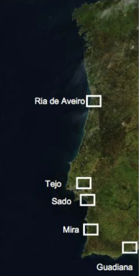
To help on the purpose of the WISER project, the fish sampling surveys conducted along several years in different estuaries (Transitional Waters) provided the database here used. To test the metrics' response against anthropogenic pressure, the survey was conducted during spring 2009 in five Portuguese estuaries (Ria Aveiro, Tagus, Sado, Mira, Guadiana) (Figure 2). Samples were collected by beam trawl, with 7-8 hauls per site, and performed at ebb tide under dark conditions.
Samples were collected inside each salinity class, following the Venice system (Anonymous 1958): oligohaline (0 – 5); mesohaline (5 – 18); and polyhaline/euhaline (> 18). The length of each beam trawl haul was calculated using the average speed and the duration or computed from the geographic coordinates of the starting and ending points of the haul. The characteristics of the sampling gear are: beam trawl; width 2 m; height 0.5 m; 5 mm mesh size in the cod end; 1 tickler chain.
Figure 2: Sampling sites. The estuaries of Ria Aveiro, Tagus, Sado, Mira and Guadiana.
CemOA
: archive
ouverte
d'Irstea
Deliverable D4.4-3
Page 14/65
2.2.2. Sample management and identification
For each fishing event, fishes were identified (whenever possible) at the species level, measured and counted. Beam trawl catches were expressed as individuals per 1000 m2. Several environmental parameters were also measured during fish surveys, at the bottom or at surface, such as the salinity, temperature, depth and oxygen saturation. Secchi depth was also recorded for some fishing events.
The fish species identification was based on the World Register of Marine Species (WoRMS) database (Appeltans et al., 2011), and was the taxonomic support for the application of the Estuarine Fish Assessment Index (EFAI) (Cabral et al., 2011). The EFAI was here used, together with other single metrics, to analyse the response of indicators (metrics and tools) against the anthropogenic pressure.
The EFAI is a recently developed methodology, compliant with WFD, which includes some metrics based on functional guilds, i.e. groups of organisms which share their biological characteristics such as nature of reproduction, feeding, spatial and temporal use of an area (Elliott and Dewailly, 1995). For the so called “ecological guilds”, “position guilds” and “trophic guilds”, which are used in several fish indices, was used a common assignment to fish species that was previously reached inside this working group (see deliverable 4.4-2 part 1). Although the original definition of the guilds came from Elliott and Dewailly (1995) and Franco et al. (2008), the WISER fish working group decided to adapt some of these ecological guilds to have them uniform for the transitional waters inside the geographical working area. These modified definitions are detailed hereafter:
Estuarine resident species (ER): when more than 50% of the population of adults and juveniles is found in transitional waters. In practical terms ER characterizes very small species that are not known to venture outside the transitional water where they reside, such as Gobiidae, Parablennius, Hippocampus, Syngnathus, etc.
Marine juvenile species (MJ): when a significant shift in juvenile distribution is observed between marine and transitional (or coastal) waters, due to a distinct migration or larval/juvenile dispersal reaching into transitional waters. In practical terms these are marine species when the majority of fishes caught in transitional waters are juveniles;
Marine seasonal species (MS): species that are entering the transitional system only at a certain periods of the year and where adults and / or juveniles are found in numbers;
Marine adventitious species (MA): when the main populations of both adults and juveniles are not found in transitional but in coastal waters. These species may be captured with regularity but numbers are low;
Diadromous species (DIA): species that cross salinity boundaries and are able to survive in freshwater and in sea water.
CemOA
: archive
ouverte
d'Irstea
2.2.3. Calculation of pressure indicators
To evaluate the response of the metrics composing EFAI, and the method itself, against anthropogenic pressure, 14 pressure indicators (Table 4) were assessed for each site to produce the site's total pressure level. In order to account for different measurement units, each pressure indicator was standardized, by its maximum and minimum values observed or possible (varying between 0-1), following Vasconcelos et al., 2007. The pressure index (Pi sum) was calculated as the sum of all pressure indicators for each estuarine site. The Aubry & Elliott (2006) adapted method (A&E) was calculated as the sum of 15 environmental integrative indicators (EII) criteria (1,2 re-alignment schemes; 1,3 land claim; 1,4 gross change in bathymetry and topography; 1,5 interference with the hydrographic regime; 2,1 Anthropogenically affected coastline; 2,4 Maintenance dredging – dredging area; 2,5a Maintenance dredging – disposal area; 2,9 Aquaculture; 2,10 fisheries causing nearshore seabed disturbance; 2,11 intensity of marina developments; 2.12 intensity of port developments; 3,1 water chemical quality; 3,2 sediment chemical quality; 3,6 shellfish quality and 3.10 interference with fish migration routes - chemical barrier), according to the values and scales defined by these authors, in order to allow direct comparisons in a common pressure scale.
Table 4. Pressure indicators used to quantify the total pressure present on each site. Type of data used and the source of information used to collect the data. EII – environmental integrative indicators; ERL – effects range low; ERM – effects range medium.
PPressure Indicators Type of data Source
Bank regulation (%) Percentage of regulated estuarine site bank length Maps/GE Dredging Mean volume and intensity Port authorities Interference hydrographic regime Percentage of area occupied by structures interfering with the hydrographic regime Maps/GE River Flow and Dams Flow (m3 s-1) and Number of large dams INAG
Sediment metals concentration Concentration & ERL and ERM Long et al. 1995 Sediment PAH concentration Concentration & ERL and ERM Long et al. 1995 Industry Number of industries in the watershed INE
Population Population density of watershed surrounding areas INE Shelfish quality Categories according to national standards IPIMAR Agriculture Used agricultural surface area INE
Aquaculture Number and area occupied IPIMAR/GE Intensity of port/marina developments Number of berths in marinas/Port areas Port authorities Commercial Fishing Number of licensed boats/Mean commercial fish landings DGPA/INE Recreational fishing Number of recreational licensed fishermen DGPA/INE Pressure index - Pi (Sum) Sum of all standardized indicators
Aubry & Elliott (A&E) adapted Adapted from 15 EII criteria
CemOA
: archive
ouverte
d'Irstea
Kruskal-Wallis- and post-hoc multiple comparisons tests). The Spearman correlation between the EFAI results and the anthropogenic pressure was analysed. Two different pressure estimations were used: a) Pressure index - Pi (sum) (local range of pressures); and b) Aubry & Elliott (2006) adapted pressure index (broader range of pressures).
2.3. Sensitivity in strength and time-lag of indices/metrics to human
pressures
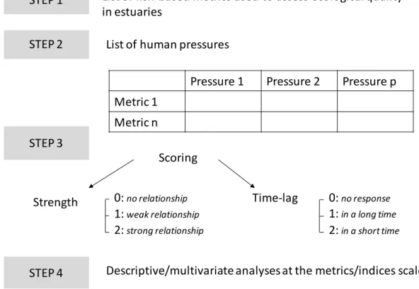
The approach chosen to evaluate the sensitivity in strength and time-lag of indices and their respective metrics to human pressures is composed on four steps, detailed in the Figure 3. Firstly, it was elaborated a list of metrics used in the different assessment indices (see Annex 1) and a list of pressures, both from literature and other bibliographic review. The list of metrics was crossed with that one of pressures (see annex 2) to score the cause-effect relationships according to its strength and time lag of response. The scores were attributed from a combination of ecological senses, published literature and expert judgement.
Figure 3. Methodology followed in the analysis of cause-effect relationships strength and time lag in response to human pressures of metrics used to assess water quality of estuarine systems based on fish assemblages.
Pressure 1 Pressure 2 Pressure p Metric 1
Metric n
STEP 1 List of fish-based metrics used to assess ecological quality in estuaries
List of human pressures STEP 2 Scoring Strength Time-lag STEP 3 0: no relationship 1: weak relationship 2: strong relationship 0: no response 1: in a long time 2: in a short time
STEP 4 Descriptive/multivariate analyses at the metrics/indices scales
CemOA
: archive
ouverte
d'Irstea
Deliverable D4.4-3
Page 18/65
2.4. Sensitivity analysis of French (ELFI) and UK (TFCI) fish indices to the
metrics dynamic range
2.4.1. Data used
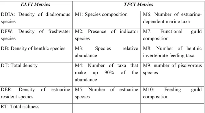
The sensitivity of fish-based indices to metric changes was investigated by using the French ELFI (Estuarine and Lagoon Fish Index) and the TFCI (Transitional Fish Classification Index). The assessment analysed a total of 68 French and 58 British transitional water bodies (WB) as defined by the WFD, covering a period between 2004 and 2010. Data were provided by IRSTEA (formerly CEMAGREF, France) and the Environment Agency (UK) and formed part of the monitoring exercise the French and UK Water Agencies are conducting for the implementation of WFD. The data were organised by water body, sampling year and by scores for the different metrics composing each index. Scores for each metric (6 metrics for ELFI and 10 for TFCI listed in Table 6) were ranked from largest to smallest.
Table 6. Definition of the acronyms of metrics forming the French ELFI and British TFCI indices
ELFI Metrics TFCI Metrics
DDIA: Density of diadromous species
M1: Species composition M6: Number of
estuarine-dependent marine taxa DFW: Density of freshwater species M2: Presence of indicator species M7: Functional guild composition
DB: Density of benthic species M3: Species relative
abundance
M8: Number of benthic invertebrate feeding taxa
DT: Total density M4: Number of taxa that
make up 90% of the abundance
M9: number of piscivorous species
DER: Density of estuarine resident species M5: Number of estuarine species M10: Feeding guild composition RT: Total richness 2.4.2. Modelling scenarios
A series of scenarios were chosen to test the sensitivity of the ELFI and TFCI indices to score changes to each of their constituent metrics. Several realistic scenarios were defined based upon the dynamic range of variation of each metric within the investigated dataset by setting each metric score to the average value observed in the 10, 40, 60, 80 percentiles (both top and low percentiles were considered), along with the average value across the entire range (all observations). The option of changing one metric at a time whilst setting the others at their average score value was considered unsatisfactory as it did not take into account relationships among metrics and hence their co-variability. These relationships were explored by using
non-CemOA
: archive
ouverte
d'Irstea
parametric Spearman-rank correlations. Based on these relationships, scenarios were defined by changing the score value of each metric and of their correlated metrics, under the assumption that metrics that are correlated with the metric driving the scenario will change more or less according to the strength of the relationship linking them. The results of the correlation tests (the correlation coefficient “ρ” and the p-value) were used to create a relationship criterion to apply when testing the sensitivity of the index to any metric manipulation (see Figures 4, 5 and 6 for details). Spearman Correlation Rho (ρ) P value Criteria Index calculated ELFI & TFCI
rho value * **
0.6 0 0.4
0.6-0.8 0.4 0.8
0.8 0.8 1
Scenarios: top & low 10, 40, 60, 80, 100 percentile of each metric Scenarios 0 0.4 0.8 1 10 100 64 28 10 40 100 76 52 40 60 100 84 68 60 80 100 92 84 80 100 100 100 100 100
Figure 4. Conceptual diagram of the approach followed to conduct the sensitivity analysis of ELFI and TFCI. Spearman correlations were calculated and a criteria was applied according to the ρ and p-values (*≤0.05, **≤0.01) of these correlations. Nine scenarios were selected to understand the behaviour of the indices towards changes in its constituent metrics (see section 2.4.3). Scenario 10 percentile (top and low) represent the more extreme manipulation and scenario 100 percentile indicates the mean value of all recorded scores. A summary of a combination of criterion and scenarios is shown in the table where the percentages needed to calculate for the related metric are shown at the different scenario levels. For example, a scenario at the 40 percentile for a given metric will mean that correlated metrics to a 0.4 level will have a value corresponding to a 76 percentile carried to calculate the index. Indices are calculated with these metric combinations and a percentage change from the average index value is computed. This percentage change is then used to create tornado and radar plots that summarize the sensitivity analysis.
CemOA
: archive
ouverte
d'Irstea
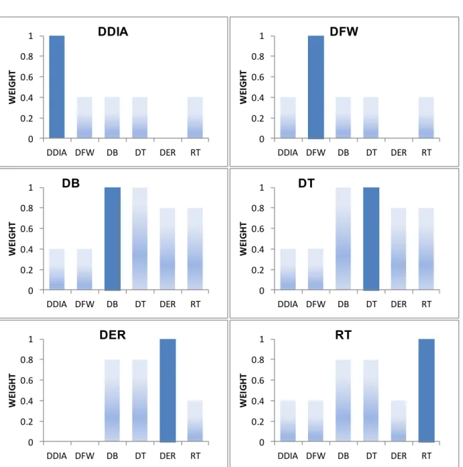
Deliverable D4.4-3 Page 20/65 0 0.2 0.4 0.6 0.8 1 DDIA DFW DB DT DER RT W EI G H T DDIA 0 0.2 0.4 0.6 0.8 1 DDIA DFW DB DT DER RT W EI G H T DFW 0 0.2 0.4 0.6 0.8 1 DDIA DFW DB DT DER RT W EI G H T DB 0 0.2 0.4 0.6 0.8 1 DDIA DFW DB DT DER RT W EI G H T DT 0 0.2 0.4 0.6 0.8 1 DDIA DFW DB DT DER RT W EI G H T DER 0 0.2 0.4 0.6 0.8 1 DDIA DFW DB DT DER RT W EI G H T RT
Figure 5. Weight applied for each metric in accordance to their correlation to the tested metric for the French index ELFI. The metric leading each scenario is indicated in the title of each graph and by the solid bar. The absence of bar indicates metrics that are uncorrelated with the metric leading the scenario (for these metrics the average score has been considered in the 4 scenario definition). CemOA : archive ouverte d'Irstea / Cemagref
0 0.2 0.4 0.6 0.8 1 M1 M2 M3 M4 M5 M6 M7 M8 M9 M 1 0 W EI G H T M1 0 0.2 0.4 0.6 0.8 1 M1 M2 M3 M4 M5 M6 M7 M8 M9 M 1 0 W EI G H T M6 0 0.2 0.4 0.6 0.8 1 M1 M2 M3 M4 M5 M6 M7 M8 M9 M10 W EI G H T M2 0 0.2 0.4 0.6 0.8 1 M1 M2 M3 M4 M5 M6 M7 M8 M9 M10 W EI G H T M7 0 0.2 0.4 0.6 0.8 1 M1 M2 M3 M4 M5 M6 M7 M8 M9 M 1 0 W EI G H T M3 0 0.2 0.4 0.6 0.8 1 M1 M2 M3 M4 M5 M6 M7 M8 M9 M 1 0 W EI G H T M8 0 0.2 0.4 0.6 0.8 1 M1 M2 M3 M4 M5 M6 M7 M8 M9 M10 W EI G H T M4 0 0.2 0.4 0.6 0.8 1 M1 M2 M3 M4 M5 M6 M7 M8 M9 M10 W EI G H T M9 0 0.2 0.4 0.6 0.8 1 M1 M2 M3 M4 M5 M6 M7 M8 M9 M 1 0 W EI G H T M5 0 0.2 0.4 0.6 0.8 1 M1 M2 M3 M4 M5 M6 M7 M8 M9 M 1 0 W EI G H T M10
Figure 6. Weight applied for each metric in accordance to their correlation to the tested metric for the British index TFCI. The figure layout is the same as in Figure 5.
CemOA
: archive
ouverte
d'Irstea
Deliverable D4.4-3
Page 22/65
2.4.3. Index response
Eight scenarios were selected to conduct the sensitivity analysis on ELFI and TFCI, from the most restrictive extreme cases (top and low 10 percentiles) to the most inclusive (top and low 80 percentile). The metric average (or 100 percentile) was calculated to express the induced change in the composite index as a percentage change from this initial value. The sensitivity analysis can be summarized using different graphing methods. One of the most informative forms are tornado diagrams where the percentage change in the index from its overall average is represented. Another way of representing the sensitivity analysis is by using radar or spider plots where the most influencing variables can be highlighted.
CemOA
: archive
ouverte
d'Irstea
3.
Results
3.1. Case study: Basque Country
3.1.1. Analysis of abiotic data
The MDS ordination plot below (Figure 7) indicates differences between estuaries based on their abiotic characteristics. For example, the Nerbioi and Lea/Barbadun represent the highest differences and therefore, the more dissimilar estuaries in terms of their abiotic (i.e. hydromorphological and pressure) characteristics.
Figure 7. Multidimensional Scaling (MDS) ordination plot, based on Bray-Curtis similarities, establishing the distances (similarities) between estuaries on the basis of their abiotic characteristics.
3.1.2. Ichthyofauna
Structural parameters
Overall, the demersal fish communities at the studied estuaries were relatively poor in terms of abundance and community composition. For example, the average abundance was 8 individuals and ranged from 0 (in several samples) to 129 (Table 7), which was recorded in the inner section of the Butroe, during the autumn survey. Similarly, species richness, Shannon’s diversity values and Pielou’s equitability values were also low. Zero values were often recorded for these parameters. Due to the high variability in the parameter values between estuaries, it was impossible to determine common patterns within/between estuary sections and seasons.
CemOA
: archive
ouverte
d'Irstea
Deliverable D4.4-3
Page 24/65
Table 7. Summary of the structural parameters for the 12 estuaries
Mean Minimum Maximum
Abundance (n) 8 0 129
Species richness (n) 2 0 9
Diversity (Shannon Index, bit ind-1) 0.68 0 2.58
Equitability (Pielou Index) 0.46 0 1
Multivariate analysis at the specific level
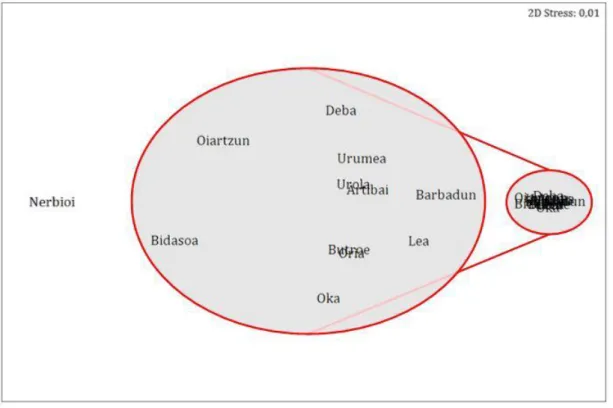
On the basis of the abundance at the different estuaries, the SIMPROF analysis defined the following statistically different estuary groups (Figure 8): 1. Oiartzun and Bidasoa, 2. Butroe and Oka, 3. Barbadun, Nerbioi, Artibai, Deba, Urola, Oria and Urumea. Lea remained independent.
Figure 8. Ordination dendrogram of estuaries, obtained from the application of a cluster analysis to averaged abundance samples and excluding seasonality of the data and estuary sector. Red colour indicates estuary groups for which abundance did not significantly differ.
Similarities and dissimilarities within and between groups (respectively) were explained by the abundance of different species rather than by the species composition (Tables 8 and 9). Hence, Group 1 (Oiartzun and Bidasoa) was defined by the abundance of Pomatoschistus sp., Gobius niger and Scorpaena porcus (Table 8). Group 2 (Butroe and Oka), on the other hand, was defined by Diplodus sargus, Pomatoschistus sp., Solea solea and Diplodus annularis, which contributed to approximately 50% of their similarities. Finally, group 3 (all other estuaries excluding the Lea) was mainly defined by species of the Pomatoschistus genus and Solea solea.
CemOA
: archive
ouverte
d'Irstea
Table 8. Abundance of specific species contributing to the similarities within estuary groups established by SIMPROF analysis. Cont: contribution of each species to the similarity between groups. Cum: Cumulative contributions.
Similarity Species Cont. (%) Cum. (%) Group 1 48.50 Pomatoschistus sp. 28.8 28.8 Gobius niger 19.6 48.4 Scorpaena porcus 14.6 63.0 Buglossidium luteum 12.5 75.5 Group 2 63.02 Diplodus sargus 20.9 20.9 Pomatoschistus sp. 15.2 36.1 Solea solea 13.9 49.9 Diplodus annularis 12.5 62.5 Gobius niger 12.0 74.5 Mugilidae 9.5 84.0 Group 3 59.63 Pomatoschistus sp. 41.3 41.3 Solea solea 30.2 71.5 Platichthys flesus 18.4 89.8
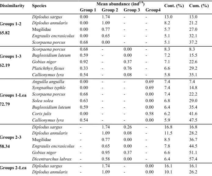
Table 9. Species that best explain dissimilarities between the estuary groups established by SIMPROF analysis. Cont: contribution of each species to the dissimilarity between groups. Cum: Cumulative contributions.
Dissimilarity Species Mean abundance (ind1/4) Cont. (%) Cum. (%) Group 1 Group 2 Group 3 Group4
- Lea Groups 1-2 65.82 Diplodus sargus 0.00 1.74 - - 13.0 13.0 Diplodus annularis 0.00 1.09 - - 8.2 21.2 Mugilidae 0.00 0.77 - - 5.7 27.0 Engraulis encrasicolus 0.00 0.65 - - 5.1 32.1 Scorpaena porcus 0.68 0.00 - - 5.1 37.2 Groups 1-3 62.19 Scorpaena porcus 0.68 - 0.00 - 8.3 8.3 Buglossidium luteum 0.59 - 0.00 - 7.2 15.5 Gobius niger 0.92 - 0.37 - 7.1 22.6 Platichthys flesus 0.33 - 0.76 - 6.6 29.2 Callionymus lyra 0.54 - 0.08 - 5.8 35.1 Groups 1-Lea 72.79 Anguilla anguilla 0.00 - - 0.69 7.4 7.4 Syngnathus typhle 0.00 - - 0.69 7.4 14.8 Scorpaena porcus 0.68 - - 0.00 7.4 22.2 Solea solea 0.63 - - 0.00 6.8 29.0 Buglossidium luteum 0.59 - - 0.00 6.4 35.4 Coris julis 0.00 - - 0.58 6.2 41.6 Callionymus lyra 0.54 - - 0.00 5.9 47.5 Groups 2-3 58.34 Diplodus sargus - 1.74 0.26 - 16.8 16.8 Diplodus annularis - 1.09 0.08 - 11.5 28.2 Mugilidae - 0.77 0.00 - 8.5 36.7 Engraulis encrasicolus - 0.65 0.00 - 7.8 44.5 Gobius niger - 0.95 0.37 - 6.6 51.1 Dicentrarchus labrax - 0.58 0.00 - 6.4 57.4 Groups 2-Lea Diplodus sargus - 1.74 - 0.00 16.1 16.1
Diplodus annularis - 1.09 - 0.00 10.1 26.2 CemOA : archive ouverte d'Irstea / Cemagref
Deliverable D4.4-3 Page 26/65 72.75 Solea solea - 1.06 - 0.00 9.6 35.8 Mugilidae - 0.77 - 0.00 7.0 42.8 Platichthys flesus - 0.74 - 0.00 6.9 49.7 Engraulis encrasicolus - 0.65 - 0.00 6.4 56.2 Anguilla anguilla - 0.00 - 0.69 6.3 62.4 Coris julis - 0.00 - 0.58 5.3 67.7 Dicentrarchus labrax - 0.58 - 0.00 5.3 73.0 Groups 3-Lea 61.93 Solea solea - - 0.85 0.00 18.1 18.1 Platichthys flesus - - 0.76 0.00 15.2 33.3 Syngnathus typhle - - 0.08 0.69 13.2 46.4 Coris julis - - 0.00 0.58 12.1 58.5 Anguilla anguilla - - 0.20 0.69 11.2 69.7 Gobius niger - - 0.37 0.76 9.7 79.5
Some of the species that best explained for differences between groups include: D. sargus, D. annularis, Mugilidae family, Engraulis encrasicolus and S. porpus. These species explained for more than 35% of the dissimilarities between groups 1 and 2, being nearly exclusive of group 2. S. porcus, Buglossidium luteum, G. niger, Platichthys flesus and Callionymus lyra explained for 35% dissimilarities between groups 1 and 3, being these species more abundant in group 1 (except for P. flesus, which is more abundant in group 3). Dissimilarities (35% level) between groups 3 and 4 were explained by Anguilla anguilla, Syngnathus typhle, S. porcus, S. solea and B. luteum. A. anguila and S. typhle were exclusive to the Lea estuary while the other three species were only identified in group 1.
Dissimilarities between groups 2 and 3 were mainly explained by higher abundances of D. sargus, D. annularis and the species of the Mugilidae family in group 2, while dissimilarities between groups 3 and 4 were primarily explained by the absence of D. sargus, D. annularis and S. solea in the Lea estuary. Finally, dissimilarities between groups 3 and 4 were explained by the fact that S. solea and P. flesus were only present in group 3. Opposite, S. typhlae was absent in group 3 and present in the Lea estuary.
Characterization of estuaries
The abiotic variables that best explained the ordination of estuaries according to biological data were: water pollution index, percentage of subtidal surface, flushing time and catchment area (BEST analysis: ρ = 0.476, p = 0.004), with water pollution index being the variable that explained most of this ordination (BEST analysis: ρ = 0.439, p = 0.007).
Considering the abiotic variables selected by the BEST analysis, LINKTREE grouped estuaries into three groups: 1. Lea and Oiartzun, 2. Oka, and 3. other estuaries (Figure 9). Lea and Oiartzun have a small catchment area (99 km2 and 86 km2 respectively, versus > 104 km2). Oka
separates from the remaining estuaries due to a flushing time, which nearly doubles that of other estuaries (149 hr versus ≥ 78 hr) and a relatively smaller subtidal area (14% versus ≤ 16%).
CemOA
: archive
ouverte
d'Irstea
Lea Oiartzun Oka Barbadun Nerbioi Butroe Artibai Deba Urola Oria Urumea Bidasoa
Figure 9. LINKTREE dendrogram based on the Bray-Curtis dissimilarity matrix of biological data and the five abiotic variables selected by the BEST analysis. SIMPROF routine was applied, which limits the number of divisions to those that are significant
On the basis of these new estuary groups, SIMPER results indicate that the Lea and Oiartzun group have relatively low similarities, which are mainly defined by Pomatoschistus sp. and G. niger (Table 10). Similarities within the other group are higher and come defined by Pomatoschistus sp. and S. solea.
Table 10. Abundance of specific species contributing to the similarities within estuary groups defined by the LINKTREE analysis. Cont: contribution of each species to the similarity within groups. Cum: Cumulative contributions.
Similarities Species Cont. (%) Cum. (%) Group 1 27.33 Pomatoschistus sp. 56.1 56.1
Gobius niger 43.9 100.0 Group 3 52.77 Pomatoschistus sp. 39.1 Solea solea 28.3 39.1 67.4
Platichthys flesus 18.6 86.0
Between estuary groups, dissimilarities were explained by the presence/absence and/or abundance of several species (Table 11). For example, D. sargus was the key species explaining for dissimilarities between the Oka estuary and the two estuary groups with a contribution of 11.9% and 12%, respectively, of the dissimilarities. Presence of P. flesus and higher abundance of S. solea in group 3 explained for most of its dissimilarities with group 1.
CemOA
: archive
ouverte
d'Irstea
Deliverable D4.4-3
Page 28/65
Table 11. Species (and their abundances) that best explain dissimilarities between the estuary groups defined by the LINKTREE analysis. Cont: contribution of each species to the dissimilarity between groups. Cum: Cumulative contributions.
Dissimilarity Species Mean abundance Cont. (%) Cum. (%) Group 1 Group 2 Group 3
Groups 1-2 68.28 Diplodus sargus 0.00 1.50 - 11.9 11.9 Diplodus annularis 0.00 0.90 - 7.1 19.0 Echiichthys vipera 0.00 0.90 - 7.1 26.1 Solea solea 0.27 1.12 - 7.0 33.1 Mugilidae 0.00 0.86 - 6.8 39.9 Hippocampus hippocampus 0.00 0.69 - 5.4 45.3 Pegusa lascaris 0.00 0.69 - 5.4 50.7 Pomatoschistus sp. 1.26 1.86 - 5.0 55.7 Groups 1-3 65.97 Platichthys flesus 0.00 - 0.76 10.5 10.5 Solea solea 0.27 - 0.85 9.4 20.0 Gobius niger 0.87 - 0.48 6.7 26.6 Syngnathus typhle 0.34 - 0.06 6.0 32.6 Anguilla anguilla 0.34 - 0.15 5.7 38.3 Coris julis 0.29 - 0.00 5.1 43.5 Groups 2-3 57.20 Diplodus sargus - 1.50 0.42 12.0 12.0 Mugilidae - 0.86 0.08 7.9 19.9 Diplodus annularis - 0.90 0.21 7.9 27.8 Echiichthys vipera - 0.90 0.14 7.4 35.2 Pomatoschistus sp. - 1.86 1.13 7.1 42.3 Syngnathus typhle - 0.76 0.06 6.9 49.2 Pegusa lascaris - 0.69 0.00 6.8 56.0 Hippocampus hippocampus - 0.69 0.07 6.2 62.2 Gobius niger - 1.03 0.48 5.8 68.0 Lithognathus mormyrus - 0.58 0.00 5.7 73.7 Dicentrarchus labrax - 0.58 0.06 5.2 78.8 Buglossidium luteum - 0.58 0.06 5.2 84.0
3.1.3. Ichthyofauna and crustaceans
Structural parameters
In line with the results obtained when analysing the ichthyofauna data alone, it was found that the demersal communities (ichthyofauna and crustaceans combined) in the estuaries were rather poor, both in terms of abundance and species richness (Table 12). For example, the inner section of the Butroe estuary (autumn season) presented the highest abundance of individuals (n = 512) versus several sites/fieldwork seasons for which only one individual was found. Despite a low average species richness value (mean = 5), individuals were homogeneously distributed within species (Pielou Index = 0.72).
CemOA
: archive
ouverte
d'Irstea
Table 12. Summary of the ichthyofauna-crustacean structural parameters for the 12 estuaries.
Mean Minimum Maximum
Abundance (n) 34 1 512
Species richness (n) 5 1 14
Diversity (Shannon Index, bit ind-1) 1.58 0 3.49
Equitability (Pielou Index) 0.72 0 1
Multivariate analysis at the species level
When considering both fish and crustaceans, the SIMPROF analysis defined two estuary groups (Figure 10): 1. Butroe and Oka, 3. Barbadun, Nerbioi, Artibai, Deba, Urola, Oria, Urumea and Bidasoa. In this case, the Lea and Oiartzun estuaries remained independent from all other estuaries.
Figure 10. Ordination dendrogram of estuaries, obtained from the application of cluster analysis to averaged abundance samples and excluding seasonality of the data and estuary sector. Red colour indicates estuary groups for which abundance did not significantly differ.
The group formed by Butroe and Oka was determined by C. crangon, C. maenas, D. sargus, P. longirostris and P. elegans, which contributed to more than 50% of the similarities between these two estuaries (Table 13). C. maenas, C. crangon, Pomatoschistus sp. and P. marmoratus
CemOA
: archive
ouverte
d'Irstea
Deliverable D4.4-3
Page 30/65
explained for more than 50% of the similarities within the other group (excluding the Lea and Oiartzun estuary).
Table 13. Abundance of specific species contributing to the similarities within estuary groups established by SIMPROF analysis. Cont: contribution of each species to the similarity between groups. Cum: Cumulative contributions.
Similarity Species Cont. (%) Cum. (%)
Gruop 1 69.28 Crangon crangon 13.5 13.5 Carcinus maenas 11.1 24.7 Diplodus sargus 9.7 34.4 Palaemon longirostris 9.2 43.6 Palaemon elegans 8.5 52.1 Pachygrapsus marmoratus 7.2 59.3 Pomatoschistus sp. 7.1 66.4 Solea solea 6.5 72.9 Diplodus annularis 5.9 78.7 Group 2 63.36 Carcinus maenas 17.8 17.8 Crangon crangon 13.4 31.2 Pomatoschistus sp. 12.6 43.8 Pachygrapsus marmoratus 11.3 55.1 Palaemon longirostris 11.2 66.3 Solea solea 9.0 75.3
The key species that defined the dissimilarity between the estuary groups are included in Table 14)
Table 14. Species that best explain dissimilarities between the estuary groups established by SIMPROF analysis. Cont: contribution of each species to the dissimilarity between groups. Cum: Cumulative contributions.
Dissimilarity Species Average abundance Cont. (%) Cum. (%) Group 1 Group 2 Lea Oiartzun
Group 1-2 46.28 Diplodus sargus 1.74 0.23 - - 9.4 9.4 Palaemon elegans 1.53 0.33 - - 7.6 17.0 Diplodus annularis 1.09 0.07 - - 6.4 23.4 Crangon crangon 2.32 1.35 - - 6.1 29.5 Mugilidae 0.77 0.00 - - 4.8 34.3 Palaemon longirostris 1.66 0.98 - - 4.3 38.6 Group 1-Lea 50.61 Diplodus sargus 1.74 - 0.00 - 10.3 10.3 Crangon crangon 2.32 - 0.86 - 8.4 18.7 Diplodus annularis 1.09 - 0.00 - 6.5 25.1 Solea solea 1.06 - 0.00 - 6.2 31.3 Palaemon serratus 0.89 - 0.00 - 5.3 36.6 Group 1-Oiartzun 69.92 Diplodus sargus 1.74 - - 0.00 5.8 5.8 Palaemon longirostris 1.66 - - 0.00 5.5 11.3 Palaemon elegans 1.53 - - 0.00 5.1 16.3 Crangon crangon 2.32 - - 1.00 4.3 20.6 Pachygrapsus marmoratus 1.30 - - 0.00 4.3 24.9 Diplodus annularis 1.09 - - 0.00 3.6 28.5 CemOA : archive ouverte d'Irstea / Cemagref
Pisidia longicornis 0.00 - - 0.90 3.0 31.5 Mugilidae 0.77 - - 0.00 2.5 34.0 Liocarcinus navigator 0.00 - - 0.76 2.5 36.5 Group 2-Lea 49.73 Palaemon elegans - 0.33 1.21 - 7.5 7.5 Solea solea - 0.84 0.00 - 7.0 14.4 Palaemon longirostris - 0.98 1.78 - 6.6 21.0 Macropodia rostrata - 0.80 0.00 - 6.5 27.6 Platichthys flesus - 0.74 0.00 - 6.2 33.7 Pilumnus hirtellus - 0.07 0.69 - 5.3 39.0 Group 2-Oiartzun 66.07 Pachygrapsus marmoratus - 1.07 - 0.00 4.9 4.9 Palaemon longirostris - 0.98 - 0.00 4.5 9.5 Liocarcinus navigator - 0.00 - 0.76 3.5 13.0 Platichthys flesus - 0.74 - 0.00 3.4 16.4 Palaemonetes sp. - 0.00 - 0.71 3.3 19.7 Arnoglossus laterna - 0.00 - 0.71 3.3 22.9 Arnoglossus thori - 0.00 - 0.71 3.3 26.2 Athanas nitescens - 0.00 - 0.64 3.0 29.2 Thoralus cranchii - 0.00 - 0.64 3.0 32.1 Buglossidium luteum - 0.07 - 0.64 2.7 34.8 Scorpaena porcus - 0.09 - 0.64 2.7 37.5 Lea-Oiartzun 73.32 Palaemon longirostris - - 1.78 0.00 7.4 7.4 Pachygrapsus marmoratus - - 1.54 0.00 6.4 13.7 Macropodia rostrata - - 0.00 1.25 5.2 18.9 Palaemon elegans - - 1.21 0.00 5.0 23.9 Pisidia longicornis - - 0.00 0.90 3.7 27.6 Palaemon serratus - - 0.00 0.76 3.1 30.8 Liocarcinus navigator - - 0.00 0.76 3.1 33.9 Palaemonetes sp. - - 0.00 0.71 2.9 36.8 Estuary characterization
The abiotic variables (hydromorphological and pressures) that best explained the assemblage of communities of the estuaries were water pollution index, total pressure index, continental shelf width, flushing time, and catchment area (BEST analysis: ρ = 0.541, p = 0.007). Out all this variables, water pollution index was the most important (BEST analysis: ρ = 0.421, p = 0.081), followed by total pressure index (BEST analysis: ρ = 0.397, p = 0.113). None of these variables alone was able to explain for the ordination of estuaries defined by their biological composition. When considering these five variables only, LINKTREE results indicate four different estuary types (Figure 11): (1) Oiartzun, (2) Lea, (3) Oka and Bidasoa and (4) the remainder estuaries.
CemOA
: archive
ouverte
d'Irstea
Deliverable D4.4-3 Page 32/65 Oiartzun Lea Barbadun Nerbioi Butroe Artibai Deba Urola Oria Urumea Oka Bidasoa
Figure 11. LINKTREE dendrogram based on the Bray-Curtis dissimilarity matrix of biological data and the five abiotic variables selected by the BEST analysis. SIMPROF routine was applied, which limits the number of divisions to those that are significant
In this case, the Oiartzun estuary was characterized by a high water pollution index (39% of the samples were polluted compared to ≤33% in other samples), a high total pressure index (2.9 vs. ≤ 2.8), and a smaller catchment basin (86 km2 vs. > 99 km2). Lea separated from the other estuaries due to its low water pollution index (4% of the samples were polluted vs. ≥8% in other samples), low total pressure index (0.8 vs. ≥0.9) and a smaller catchment basin (99 km2 vs. >104
km2). Finally, Oka and Bidasoa were characterized by a shorter continental shelf width (<16 km) than that of all the estuaries encompassed in group 4.
Having defined these four estuary types, species that characterized the demersal communities of these estuary groups (fish and crustaceans species and abundances) were determined and are now presented on Tables 15 and 16.
CemOA
: archive
ouverte
d'Irstea