Distant Hemodynamic Impact of Local Geometric
Alterations in the Arterial Tree
by
Yoram Richter
B.S. Physics and Computer Science Tel Aviv University, 1997
Submitted to the Department of Electrical Engineering and Computer Science in partial fulfillment of the requirements for the degree of
MASTER OF SCIENCE IN ELECTRICAL ENGINEERING AND COMPUTER SCIENCE
AT THE
MASSACHUSETTS INSTITUTE OF TECHNOLOGY JUNE 2000
2000 Massachusetts Institute of Technology _
All rights reserved MASSACHUSETTS INSTITUTE
OF TECHNOLOGY
LIBRARIES
Signature of Author _
Department of Electrical Engineering and Computer Science May 19, 2000
Certified by
Elazer R. Edelman Thomas D. and Virginia W. Cabot Associate Professor -Division of Health Sciences and Technology The5is Supervisor Accepted by
-Arthur C. Smith Professor of Electrical Engineering and Computer Science Chairman, Committee on Graduate Students
MASSAHEUS INsTIL
Distant Hemodynamic Impact of Local Geometric
Alterations in the Arterial Tree
by
Yoram Richter
Submitted to the Department of Electrical Engineering and Computer Science on May 19, 2000 in Partial Fulfillment of the Requirements for the Degree of
Master of Science in Electrical Engineering and Computer Science
ABSTRACT
Hemodynamics has long been identified as a major factor in the determination and localization of atherosclerotic lesions. Atherosclerosis is focal and often forms in specific locations in the arterial tree such as bifurcations. Many different aspects of fluid mechanics have been suggested as the trigger for atherogenesis - non-laminar and/or unstable flow, flow separation, regions of higher/lower and/or oscillatory shear stress etc. While the precise mechanism by which these hemodynamic factors act is not yet clear, the fact that they correlate highly with atherogenesis suggests that local disturbances in flow through blood vessels can promote arterial disease. These issues have become increasingly acute as physicians seek to alter the pathological arterial anatomy with bypass grafting or endovascular manipulations such as angioplasty or stenting.
We proposed that vascular interventions might cause previously unforeseen effects in the arterial tree especially at branch points. Manipulation of one branch of a bifurcation might adversely affect the contralateral branch of the bifurcation. The goal of this work was to study the distant impact of local flow alterations, as well as to classify and evaluate the different parameters that determine their severity. Dynamic flow models of the arterial system were developed that allowed for the continuous alteration of model geometry in a controlled fashion. This property allows for the simulation not only of the healthy or diseased states, but also of the entire range in between. Moreover, these models permit simulation of different strategies of clinical intervention. Flow through the models was investigated using both qualitative (flow visualization) and quantitative (flow and pressure readings) tools. Flow separation and vascular resistance in one location of the arterial tree varied with geometrical alterations in another.
The results of this study could have important implications for the diagnosis, treatment and long-term follow-up of the large number of patients who suffer from these diseases and undergo vascular interventions. Clinical arterial manipulation of one arterial site may well need to consider the hemodynamic impact on vascular segments at a distance.
Thesis Supervisor: Elazer R. Edelman
Acknowledgements
Elazer Edelman. For proving everyday that you can mix clinical practice and quality research, family and career, religion and science, personal academic achievements and true mentoring, oil and water, teacher and friend.
Tom McMahon. If it wasn't for his generosity, experience and technical creativity this project might well have remained no more than wishful thinking. He will sorely be missed.
My mother. God only knows how she put up with me for so long, but everything I am
today, for better or worse, is the direct result. My father. For never telling me what he thought I should do and yet providing the guidance to make the choices so easy, obvious and clear. By their profound achievements - family, academic, business and
humanitarian - they define the word synergism.
Table of contents Acknowledgements 3 Table of contents 4 List of figures 6 List of tables 7 Chapter 1: Introduction 8 I. General 8
II. Relationship of atherosclerosis to fluid mechanics 8
III. Modalities of treatment 12
IV. Prior work 13
V. Time course of disease and response to treatment 15 VI. Interactions between different sites in the arterial tree 15
VII. Experimental scenario 17
VIII. References 22
Chapter 2: Materials and methods 24
I. Fabrication and operation of mock circulation 24
1.1 Creation of solid cast 25
1.2 Fixation of cast and embedding in silicone 27
1.3 Melting and connections 30
II. Instrumentation and analysis 31
11.1 Flow circuit 31
11.2 Flow waveform acquisition 32
11.3 Pressure waveform acquisition 33
11.4 Waveform conditioning and synchronization 35
III. General flow visualization 37
111.1 Formation of Tracer particles 37
111.2 Filming/image acquisition 38
111.3 Image enhancement 38
IV. Dimensionless analysis 40
V. Derivation of parameters for model circulation 46
VI. References 49
Chapter 3: Experiment 50
I. Experiment 1 - Establishment of flow regime 51
1.1 Theory 51
1.2 Experiment 54
1.3 Results and Discussion 55
II. Experiment 2 - Mathematical modeling 57
11.1 Theory 57
11.2 Experiment 58
III. Experiment 3 - Flow visualization
111.1 Theory
111.2 Experiment
111.3 Results and Discussion
IV. Experiment 4 - Sedimentation analysis IV.1 Theory
IV.2 Experiment
IV.3 Results and Discussion V. References
Chapter 4: Conclusions
I. Inertance dominated flow
II. Mathematical modeling III. Flow visualization IV. Sedimentation analysis V. Future work
Appendix A: Design and operation of sensors Appendix B: Code 65 65 69 70 87 87 89 89 96 97 97 98 99 101 102 104 107
List of figures
Figure 1-1: Simple electric analogy for flow 16
Figure 1-2: Flow through a simple bifurcation 18
Figure 1-3: Flow through a tapering bifurcation 19
Figure 1-4: Flow through bifurcation with lesion in daughter branch 20 Figure 1-5: Dilation of daughter branch 21
Figure 2-1: Flow model 24
Figure 2-2: Operation of "push-pull plungers" 25
Figure 2-3: Wax casts 26
Figure 2-4: Suspension of wax cast prior to polyurethane pouring 26
Figure 2-5: Glass interface pieces 28
Figure 2-6: O-ring effect 28
Figure 2-7: Interface sealing 29
Figure 2-8: Fixation of PEG cast 29
Figure 2-9: Model after curing of silicone 30
Figure 2-10: Proximal ports 31
Figure 2-11: Distal tubing and reservoirs 32
Figure 2-12: Flow sensor 33
Figure 2-13: Differential pressure sensor 34 Figure 2-14: Proximal pressure measurement using differential pressure sensor 34
Figure 2-15: Pressure wire insertion 35
Figure 2-16: Waveform synchronization 37
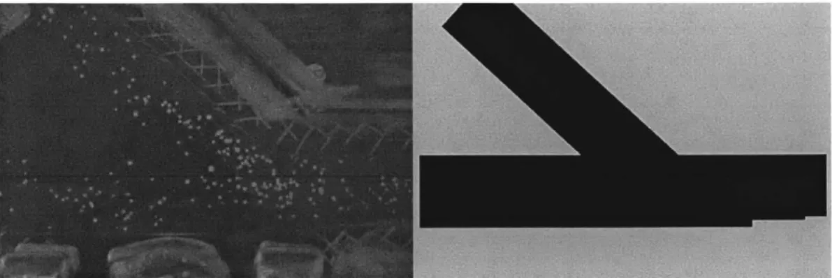
Figure 2-17: Mask image 39
Figure 2-18: Image enhancement 39
Figure 2-19: Instantaneous flow profiles for different Womerseley numbers 44 Figure 3-1: Proximal pressure tap for differential pressure measurement 54 Figure 3-2: Fourier transform of waveforms and impedance 55
Figure 3-3: Effective diameter in a tube with separated flow 58
Figure 3-4: Waveform acquisition 60
Figure 3-5: Waveform simulation 60
Figure 3-6: Quantification of resistance 62
Figure 3-7: Scheme for creating composite images for PIV 68
Figure 3-8: Case 10 visualization 71
Figure 3-9: Case 11 visualization 74
Figure 3-10: Case 12 visualization 76
Figure 3-11: Case 13 visualization 77
Figure 3-12: Case 14 visualization 79
Figure 3-13: Collateral steal 80
Figure 3-14: Case 15 visualization 81
Figure 3-15: Case 16 visualization 83
Figure 3-16: Case 17 visualization 84
Figure 3-17: PIV at different time points 86
Figure 3-18: Case 10,11 sedimentation patterns 90
Figure 3-19: Case 12,13 sedimentation patterns 91
Figure 3-20: Case 14,15 sedimentation patterns 92
Figure 3-21: Case 16,17 sedimentation patterns 93
List of tables
Table 2-1: Reynolds numbers 43
Table 3-1: Experimental cases for quantification of flow separation 59
Chapter 1: Introduction
I. General:
The examination of the potential impact of hemodynamics and atherosclerosis has been coupled for some time. The hallmark of atherosclerotic vascular disease, the
gradual occlusion of a blood vessel's cross section, is altered flow. As atherosclerotic vascular disease is the leading cause of mortality and morbidity around the world, many have sought to understand how atherosclerotic lesions, form, grow and destabilize based on fundamental fluid dynamics. This work proposes an alternative means of analyzing the types of fluid dynamic interactions that could contribute to atherosclerotic disease.
II. Relationship of atherosclerosis to fluid mechanics:
Early workers in the field of atherosclerosis research noticed a unique phenomenon: Despite the systemic factors such as tobacco abuse, hypertension, and diabetes that place patients at risk of developing atherosclerosis, the distribution of atherosclerotic lesions is far from uniform and often predictably localized to specific regions of the arterial tree1. Regions in and around bifurcations2 and bends in the arterial
tree have a considerably higher atherosclerotic plaque burden than other locations even those only one or two diameters away. These observations, have led to the school of thought that attributes at least part of the disease to fluid mechanic stimuli3. Since the
properties of flow patterns change quite considerably over the relevant length scales, it seems appropriate to attribute the progression of disease and especially the early part which would determine it's localization to the interplay of forces and flows between the blood flowing in the arteries and the arterial wall.
Whatever the flow pattern in the vessel is, the actual transduction of force to the vessel wall is through the shear stress, which is by definition the force per unit area exerted by the fluid on the vessel wall. It is thus reasonable to begin to look for
potentially deleterious flow patterns in those that produce abnormalities in shear stress4. The importance of shear is further reinforced by the concentration of atherosclerotic plaque in regions of the vascular bed that have abnormally high and low shear stress, bifurcations.
Several characteristics of flow have been proposed over the years as a stimulus for the development of atherosclerotic disease. It was initially proposed that abnormally high shear stress cause disruption damage and denudation of the endothelial cell layer1,5.
Endothelial dysfunction is a primary factor in the initiation and propagation of
atherosclerotic lesions. Yet, examination of the bifurcations themselves shed light on this theory. Bifurcations possess regions of abnormally low and high shear stress, the highest values being found around the flow divider region. However, it is the high shear regions of bifurcations that are typically spared of the common elements of atherosclerosis including lipid deposits, inflammatory cells, fibrosis, etc.
Thus, rather than a specific shear event, turbulent flow patterns6,7 were thought
to explain the observed localization of lesions, through damage to the endothelium as well, and deposition of different blood-borne products onto the vessel wall. The difficulty is that it is rare to encounter conditions under which laminar flow becomes turbulent within the arterial bed. Arterial flow rates do vary but in general the Reynolds numbers, are well below the upper critical value at which laminar flow can be expected to turn turbulent, and are typically less than the lower critical Reynolds number at which
turbulence is expected to die out and revert to laminar flow. Thus, while turbulence might exist at very specialized locations, for example immediately downstream from heart valves and in some locations in the ventricles, as a general rule turbulence would not be expected to prevail in the arterial bed, and certainly not to the extent that would explain the wide distribution of atherosclerotic disease8.
Given these facts, the focus has shifted from high shear regions to low shear regions9-1 1. Low shear can abrade the endothelium and directly affects gene expression patterns and the function of endothelial cells121 3. A bifurcation can exhibit several
regions of lower shear stress. Most prominent of these are the two regions of boundary layer separation that exist in the lateral angles of the bifurcation1 4. Stretching from
stagnation point to point of reattachment, these two areas are ones in which the shear stress is abnormally low throughout. This has led several workers to suggest a direct link between localization of atherosclerosis and regions of boundary layer separation15. Other
features of the flow in separated regions have also been proposed as possible promoters for atherogenesis, these include both reverse and pulsatile (non-uniform) shear stress and have been shown to correlate with the localization of atherosclerotic plaques in vivo16.
The importance of low shear stress is consistent with the evolving view of
atherosclerosis as an inflammatory process17, wherein the progression of atherosclerosis
is governed by a series of reactions between the vessel wall and a multitude of blood-borne inflammatory cells, particles and proteins. The characterization of these reactions and the factors that determine their progression is a complex science. However, one must keep in mind that the interaction of the inflammatory cells with the vessel wall does not happen in a vacuum. Rather, throughout these events the inflammatory cells and the vessel wall itself are subjected to varying forces exerted on them by the arterial architecture and flowing blood. These forces will determine to a large extent the
properties of the endothelial lining through which the inflammatory cells must traverse, the forces acting on them as they attempt to breach the vessel wall and indeed which and how many cells arrive at any given location to begin with.
This view of atherosclerosis lends itself especially well to the relation of fluid mechanic phenomena, particularly low shear stress and boundary layer separation, to atherogenesis and the progression of atherosclerotic disease. The process of inflammatory cell penetration of the endothelial cell layer is not an instantaneous one by any means. Rather, it is a gradual, multi-stage process that takes place over numerous cycles of flow. Throughout this process, the cells are subjected to forces exerted on them by the vessel wall, by adjacent cells and also by the flowing blood. At least in the initial stages, the
adherence of these cells is passive and thus whether or not the cells eventually bind and penetrate the vessel wall, or on a global scale, the probability and hence the number of cells which ultimately breach the vessel wall, is determined by the balance of forces that bind cells, and those forces which would tear them away. These latter forces, which retard penetration of the vessel wall, are no more than an expression of the shear stress, would be reduced in regions where for whatever reason the shear stress is abnormally low. Furthermore, regions of boundary layer separation, which include re-circulating and sluggish flows, would increase residence times for the inflammatory agents near the vessel wall. This would allow more time for the reactions to occur and reach the point
where the cells take on a more active migratory nature and contribute further to the progression of atherosclerotic disease.
Other more detailed models of the interactions of flow with the arterial wall have focused on oscillatory, bi-directional and spatially and temporally alternating flow patterns16. One could easily make a link between atherogenesis and any altered flow pattern. Endothelial cells have been shown to be adapted to the local flow conditions that they encounter. One example of this type of adaptation is the morphologic appearance of these cells1 8. Cells that are subjected to high, yet physiologic, flows tend to have an
elongated appearance when viewed en-face, with the long axis oriented along the
direction of flow. Conversely, cells that are subjected to more static conditions tend to be more rounded18. In a system as intricately evolved as this, it seems reasonable to assume
that endothelial cells are specifically suited to whatever the flow conditions at their location happen to be. Assuming this to be the case, one would expect that any alteration in the flow pattern, be it direction, velocity, a higher or a lower shear stress or any other change from what the cells in that particular location have been conditioned for, would have a negative effect on endothelial cell function.
Whatever the mechanism of action, one cannot ignore the simple
phenomenological correlation between regions of boundary layer separation and
development of atherosclerotic disease. Some studies19 have gone as far as showing not
only a one-to-one correlation in the localization of these two factors, but actually a striking resemblance in the physical shape of the region of separation and the subsequent atherosclerotic lesion that develops. This resemblance is so extensive, especially around bends and bifurcations, that one is led to think of mechanisms whereby the separated
flow triggers atherogenesis, and the lesion develops until it fills the entire original space taken up by the separated flow. It is these observations that prompted the present work to focus on boundary layer separation. An implicit assumption is made, that any process that tends to reduce the extent of flow separation is beneficial, whereas any process that tends to enlarge it is deleterious in its effects.
III. Modalities of treatment:
The end result of the long course of vascular disease will in most cases be luminal
occlusions that jeopardize organ perfusion to such an extent as to necessitate corrective or bypass procedures. It is worthwhile noting that these luminal occlusions need not be complete, or nearly complete to exert a significant effect on the organ. One explanation for this fact lies in an appreciation of the fluid mechanic principles involved. As will be discussed later, the resistance to flow of an arterial segment' is under ideal situations inversely related to the fourth power of the diameter of the segment. Thus, even a modest decrease in diameter can have a drastic effect on the resistance to flow of the artery, and hence the amount of blood which it delivers. A second explanation has to do with the morphology and natural history of atherosclerotic lesions. Some lesions may, at certain points become unstable and rupture, exposing cells and tissues and releasing agents to the
circulation with dramatic effects. There is evidence that the unstable lesions that rupture are less likely to be the ones that present a substantial luminal occlusion or reduction in cross-sectional area.
Corrective procedures might take the form of bypass grafting or angioplasty e.g. from percutaneous procedures known as Percutaneous Transluminal Angioplasty (PTA). During bypass grafting, an alternative flow channel" is used to divert flow from a point upstream or proximal to the lesion to a point on the vessel that is downstream or distal to the lesion. During angioplasty, the artery is dilated to approximate its original dimensions and flow is restored downstream in the vessel.
The long term efficacy and benefit of these procedures is a topic of intense investigation and debate. The relative advantages and disadvantages of one procedure over the other are of tremendous clinical importance but also in many cases unclear. Regardless, the most common mode of failure of these two treatment modalities is similar
- accelerated occlusion of the new flow channel. In the case of bypass grafting this is
The resistance to flow is inversely related to the amount of flow going through the segment in a parallel circuit such as the arterial tree.
" The sources for this channel are numerous and include the saphenous vein from the leg, the radial artery
from the arm and the internal mammary artery from the chest, as well as research efforts into artificial sources.
commonly referred to as graft occlusion, whereas in the case of angioplasty this is known as restenosis.
IV. Prior Work:
A large body of experimental evidence has been assembled regarding the flow in
different parts of the arterial tree and especially that which exists in and around arterial bifurcations. This work includes analytical analysis, modeling by use of mock circulation
systems as well as numerical analysis. Each one of these approaches has its advantages and its limitations:
Analytical work is the most precise and can give perhaps the most insight and intuition into the problem. Unfortunately, the full Navier-Stokes equation that governs flow in the relevant regime of intermediate Reynolds numbers is complex and can only be solved analytically for a handful of highly simplified geometries. This leaves the latter two methods - numerical analysis and physical modeling. Of these two, numerical analysis is clearly the more flexible as it allows for changing of the parameters that characterize the problem virtually instantly. However, numerical analysis is of lesser accuracy at the singular points of flow unsteadiness and separation20. Since these are the points at which
the phenomena of interest here occur, this presents a severe limitation to the applicability of the results. The second limitation of numerical analysis is that while it is for the most part well suited for the solution of partial differential equations which govern the flow, it runs into great difficulties in predicting things such as the particle sedimentation patterns in these flows, as these problems include an inherent stochastic element. Physical
modeling is a highly refined method dating back at least 1872 when William Froude built the first towing tank to test the resistance of ocean vessels. It is however not without its own limitations, the major ones being the fact that it is time consuming, the relative difficulty associated with altering the parameters modeled and the inherent inaccuracies stemming from physical limitations of the modeling apparatus.
Since the central role of bifurcations was identified early on, analytical2 1,
numerical2 0,22-24 and physical modeling1 9,2 5-2 7 methods have all been employed to
the analysis of bifurcations. Typical sites examined have been the left main coronary bifurcation2 2, the carotid bifurcation2 7, the pulmonary artery bifurcation2 8 and the main
aortic bifurcation. Experiments typically map different flow parameters in the region such as flow vectors, pressure gradients, shear rates and shear stresses along the artery wall as well as others. While extensive, these models all share several common characteristics. This set of common characteristics coincides with a resultant shared set of limitations, which shall be discussed hence.
Past models have all been similar in that they:
a) usually simulate conditions in healthy arteries, that is, before lesions have actually formed2 2.
b) are often highly specialized to specific situations such as a T-bifurcation, a symmetric
bifurcation etc. To mimic the specific case in question input flow parameters, such as flow rate and pressure profile, and the physical properties of the model, e.g. relative diameters, bifurcation angles etc. are determined as precisely as possible1 9,2 0,2 6.
c) concentrate on what has been perceived as the "causal" effects, i.e. the effects distal to the bifurcation in one specific independent branch.
d) are "static", modeling the system at one point in time, and do not allow for the long
term remodeling of the system that occurs in the natural case2 5.
These common features also provide a set of respective limitations to their applicability: a) While providing valuable insight into the process of atherogenesis, and helping to
explain areas of high risk, this type of work is of limited clinical application. High-risk areas may be identified but clinical intervention before significant lesions have occurred is unlikely.
b) Since each actual clinical case is unique, the value and applicability of a highly
specialized model is severely limited. That is to say that the chances in any one clinical setting that the geometrical attributes of a patient's disease will coincide with a case which has been modeled are extremely remote. For this reason, the knowledge gained has had a limited effect on the practices of clinicians presented with a wide range of specialized cases but no concise set of general guidelines.
c) Models that examine only down-stream vessels ignore the potential impact on the
larger and possibly more clinically important proximal vessels.
d) Static systems ignore the long-term dynamic nature of the arterial system, which
V. Time course of disease and response to intervention:
An important issue to appreciate is the time course of the different processes
involved in atherosclerotic disease. The progression of the disease itself is quite slow. Precursors of atherosclerotic lesions can readily be identified in healthy individuals in their early twenties. Observations have been made of fatty streaks, the very earliest form of atherosclerotic lesions, in children as young as two to four years of age. However, normal adults' do not typically become symptomatic until their mid to late fifties. The natural progression of atherosclerotic lesions is a slow and gradual one, taking anywhere from thirty to fifty years and perhaps even longer to develop.
The changes in the arterial wall imposed by bypass or angioplasty are entirely different however. These changes take place over the course of what amounts to minutes to hours. The response of the tissue to these rapid changes can be expected to vary greatly from that to the disease itself. A system that has been designed to deal optimally with events that occur over the course of many years in an optimal manner can be expected to react in a sub-optimal and perhaps even deleterious manner to changes on this vastly shorter time scale. One possible manifestation of this effect might be restenosis, which runs on a much shorter time scale of months to years as opposed to the decades over which the original disease developed. When considering the effects of interventions it is thus helpful to view the arterial system as one that is normally in a quasi-steady state very close to equilibrium, and has suddenly been thrust much further away from the
equilibrium point than it would normally be.
VI. Interactions between different sites in the arterial tree:
In the clinical setting, lesions in individual arteries have typically been treated as separate and independent events. While the presence of lesions in multiple sites is certainly an indication for choosing one type of treatment modality over another, the continued progression of lesions in segments that were not manipulated has not been attributed to interactions between these sites, but rather to the underlying systemic disease manifesting itself in several locations. Similarly, the occurrence of lesions, either
By normal here we mean ones that do not suffer from diabetes mellitus or any other form of genetic or
de-novo or as a progression of prior ones, over time has typically not been attributed to a causal relationship between them or to a result of an intervention but rather further symptoms of an already established disease.
Consequently, the treatment of lesions has been on an individual basis with little regard to the effects that treatment of one site might have on another. Furthermore, the long-term follow-up of patients who were treated with one form of intervention or
another has focused on the site at which the intervention was performed. A demonstration of this point is the fact that one of the most common criteria for the evaluation of efficacy of a treatment modality over time is the rate of "target lesion revascularization".
The basis of this thesis is the assertion that this view is an oversimplification of the problem. The reasons for this assertion can be broken down into three main factors:
1. We first examine a vastly oversimplified analogy for a fluid flow circuit - that of a completely passive electrical circuit:
Figure 1-1: Simple electric analogy for flow
In this analogy, a lesion in a branch is simulated by raising the resistance of the appropriate resistor. Re-adjusting the value of the resistance down towards its original value simulates dilation of this lesion. Clearly, any change in the resistance on one branch will have an effect on not only the flow in that branch but also on the flow through the contralateral one.
2. In the case given above, each flow branch is modeled by an entirely passive circuit element. In reality, the case is much more complex: Each vessel segment posses a fluid dynamic impedance, which is a generalized dynamic resistance taking into account the compliance of the vessel, the inertia of the fluid and the frequency of oscillations. This impedance is different from the circuit above in that while electrical resistors have set impedance regardless of the circuit they are placed in, the impedance of a vessel is
dependant on the flow patterns it is subjected to. Any change in one part of such a circuit will necessarily effect a change in the flow patterns through other parts of the circuit and hence change the impedance of these other channels thus altering the flow patterns
further. In this manner, a complex interaction is set up between any part of the flow circuit and all other parts.
3. Real arteries are composed of living tissue and are not simply solid tubes. They have
the capacity to adapt and react to changing flow conditions. It is the assumption of this work that under normal conditions, these adaptations optimize the entire flow system from the perspective of some crucial parameter such as energy consumption or tissue perfusion. Under abnormal conditions there could be a derailment of these adaptive mechanisms and adverse results.
Regardless of what guides these adaptations, the end result is that intervention on one site might under certain conditions set off a host of adaptive responses in other sites. As the effects are fluid dynamic, the impact may be observed downstream from the site of intervention, upstream from it, or in a parallel flow channel. Some of these
interventions might trigger a problem of considerably larger implications than that which they attempted to solve, for example if an intervention in one site has an adverse effect on a more proximal vessel. In other, less extreme cases, the type of intervention and the manner in which it is performed would surely benefit from a more complete
understanding of the interactive processes involved so as to produce a more favorable long term result.
VII. Experimental scenario:
To demonstrate this approach, a specific clinical scenario was outlined to simulate
the progression of disease, the clinical intervention performed and the possible long-term outcomes. It is crucial to note that this scenario in no way attempts to model the most prevalent clinical situation. Nor does it attempt to model precisely any specific type of
intervention. In fact, no attempt has been made to accurately model any real-world situation at all. The sole purpose of the scenario is to provide a framework through which the types of interactions discussed can be examined individually and their impact
precisely analyzed and rigorously demonstrated. This scenario is the backbone of the set of experiments performed:
1. Basic bifurcation geometry:
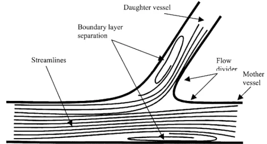
The basic geometry of a bifurcation includes an inherent fluid mechanics problem. On a theoretical basis alone one would expect two regions of flow separation to form (see fig. 1-2). The first region forms in the ostium of the side branch. This separation can be understood in several ways but perhaps the most intuitive is the point of view of inertia. That is to say that the blood flowing down the main branch simply has too much inertia to negotiate the sharp bend on the lateral wall of the bifurcation. The second region of separation forms in the main branch' facing the ostium of the side branch. This can be understood in several ways: One is to think of it as a result of the take-off of blood into the side branch that diverts all streamlines away from the wall. This is however somewhat misleading as it predicts that at a zero degree angle of bifurcation - the case in which one channel simply divides into two parallel channels
- one would not see this region of separated flow - a result that is false2 1. Perhaps the more correct way of thinking of this region of separation is to consider the flow in the main branch against an adverse pressure gradient created by the imposition of a new boundary layer - that which forms along the flow divider.
Daughter vessel Boundary layer separation Streamlines Flow divider Mother vessel
Figure 1-2: Flow through a simple bifurcation - regions of boundary layer separation.
During the course of this thesis we will be using the terms "main branch" and "mother branch" and the terms "side branch" and "daughter branch" interchangeably.
2. Tapered bifurcation:
In reality, major bifurcations' do not normally appear as in fig. 1-2. Rather, most bifurcations include a tapering of the lateral wall of the mother branch from approximately the point that faces the ostium of the daughter branch. This is demonstrated in fig. 1-3.
Figure 1-3: Flow through a tapering bifurcation
One possible explanation for the benefit of this geometry is that by approximating the curvature of the streamlines with the vessel wall itself, the artery reduces or perhaps eliminates the region of flow separation in the main branch. Note however that the region of separation in the side branch still exists, as approximating the streamlines with the vessel wall at this point would severely reduce the diameter of the daughter branch. This is indeed where most of the lesions in bifurcations actually occur.
3. Lesion in daughter vessel:
Flow separation in the ostium of the daughter vessel produces, a lesion. Because the progression of disease is very gradual, the system has time to react adaptively to the slow occlusion of the side branch. This can be done in a number of ways including alterations in the downstream resistance i.e. the vascular bed, development of
collateral circulation (see fig. 1-4) as well as shifting of the input flow patterns to the system itself (by shunting flow away from other sites for example). Whatever these adaptations turn out to be, the original cause of boundary layer separation in the
The term "major" refers to those bifurcations where the diameter of the daughter branch is not insignificant with respect to the diameter of the mother branch.
mother vessel, take-off of flow at the bifurcation, no longer exists. The tapering of the mother vessel now serves no advantageous role and is actually detrimental as it needlessly increases the resistance to flow of the mother branch. It is reasonable to assume then that the system will adapt in such a way as to eliminate this tapering. It is even conceivable that due to the increased pressure in the region of the bifurcation the artery might actually bulge out at this point (see fig. 1-4).
Collateral
vessel Lesion
Figure 1-4: Flow through bifurcation with lesion in daughter branch. Note development of collateral circulation as well as the elimination of taper in the mother branch facing the ostium.
Note that in this new configuration boundary layer separation has been minimized, perhaps eliminated. There is of course still a perfusion problem to the region that was
served by the daughter vessel. 4. Dilation of daughter branch:
The assumption made when dilating a lesion is that one is returning the system to its original configuration. If however we take into account the fact that the system has adapted to the changing conditions over the course of the disease as it has here, it becomes clear that by dilating the lesion one actually creates a completely new configuration. In this new configuration, the other parts of the system are no longer optimized for the conditions with which they are presented and one possible
manifestation of this could be the re-establishment of a region of separation in the main branch as depicted in figure 1-5. In other words, restoration of the original anatomy or vascular architecture may not restore the initial or optimal flow conditions.
Figure 1-5: Dilation of daughter branch. Note formation of new area of boundary layer separation in mother branch due to non-optimized flow.
At this point, one must consider the previous discussion of time scales. A system which normally reacts to changes in the flow regime that take place over the course of years to decades, is now presented with a vast alteration in flow over the course of minutes to hours. The biological reaction to such a change can be expected to be different from the
controlled normal reaction. Rather, the system might react in an uncontrolled manner to produce a lesion in the main branch rather than stopping at a mild taper.
The experiments outlined in this thesis track this general scenario and
demonstrate the properties of flow at each stage. Flow is analyzed using several different tools to both verify the theoretical predictions made above, and to attempt to predict what their implications might be. This is done in a manner that does not attempt to be true to any specific set of parameters measured in a real case, or even those indicated by taking an average of all cases. Rather, it is performed in a generalized manner so as to attempt to tease out the underlying qualitative rules that govern these processes regardless of the data pertaining to the individual case.
Chapter 2 outlines the methods by which the flow model was built and analyzed. Chapter 3 presents the experiments performed and analyzes the results obtained. Chapter 4 contains conclusions and suggestions for future work.
VIII. References:
1. Texon M. A Hemodynamic Concept of Atherosclerosis, with Particular Reference to Coronary
Occlusion. A.M.A. Archives ofInternal Medicine. 1957;99:418-427.
2. Roach MR. The effects of bifurcations and stenoses on arterial disease. In: Cardiovascularflow
dynamics & measurements. Baltimore: Park Press; 1977.
3. Giddens DP, Zarins CK, Glagov S. The role of fluid mechanics in the localization and detection of
atherosclerosis. Journal of Biomechanical Engineering. 1993; 115:588-594.
4. Krams R, Wentzel JJ, Oomen JAF, Vinke R, Schuurbiers JCH, De Feyter PJ, Serruys PW, Slager
CJ. Evaluation of Endothelial Shear Stress and 3D Geometry as Factors Determining the
Development of Atherosclerosis and Remodeling in Human Coronary Arteries in Vivo.
Arteriosclerosis Thrombosis and Vascular Biology. 1997; 17:2061-2065.
5. Fry DL. Acute Vascular Endothelial Changes Associated with Increased Blood Velocity
Gradients. Ciculation Research. 1968;22:165-197.
6. Fergusson GG, Roach MR. Flow Conditions at Bifurcations as Determined in Glass Models with
Reference to the Focal Distribution of Vascular Lesions. In: Bergel DH, ed. Carsiovascular Fluid Dynamics. Orlando.: Academic Press Inc.; 1976:141-157.
7. Gutstein WH, Farrell GA, Armellini C. Blood flow Disturbance and Endothelial Cell Injury in
Pre-Atherosclerotic Swine. Laboratory Investigation. 1973;29:134-149.
8. Glagov S, Zarins C, Giddens DP, Ku DN. Hemodynamics and Atherosclerosis. Insights and
Perspectives Gained From Studies of Human Arteries. Archives ofPathology and Laboratory Medicine. 1988;112:1018-1031.
9. Friedman MH, Deters OJ, Bargeron CB, Hutchins GM, Mark FF. Shear-Dependent Thickening of
the Human Arterial Intima. Atherosclerosis. 1986;60:161-171.
10. Sabbah HN, Khaja F, Brymer JF, Hawkins ET, Stein PD. Blood Velocity in the Right Coronary
Artery: Relation to the Distribution of Atherosclerotic Lesions. American Journal of Cardiology.
1984;53:1008-1012.
11. Gibson MC, Diaz L, Kandarpa K, Sacks FM, Pasternak RC, Sandor TS, Feldman C, Stone PH.
Relation of Vessel Wall Shear Stress to Atherosclerosis Progression in Human Coronary Arteries.
Arteriosclerosis and Thrombosis. 1993; 13:310-315.
12. Davies PF. Mechanisms involved in endothelial responses to hemodynamic forces.
Atherosclerosis. 1997;131 Suppl:S15-7.
13. DePaola N, Gimbrone MAJ, Davies PF, Dewey CF. Vascular endothelium responds to fluid shear
stress gradients. Arteriosclerosis & Thrombosis. 1992; 12:1254-1257.
14. Fernandez RC, De Witt KJ, Botwin MR. Pulsatile Flow Through a Bifurcation with Applications
to Arterial Disease. Journal ofBiomechanics. 1976;9:575-580.
15. Fox JA, Hugh AE. Localization of Atheroma: A Theory Based on Boundary Layer Separation.
British Heart Journal. 1966;28:388-399.
16. Moore JE, Xu C, Glagov S, Zarins CK, Ku DN. Fluid wall shear stress measurements in a model
of the human abdominal aorta: oscillatory behavior and relationship to atherosclerosis.
Atherosclerosis. 1994; 110:225-240.
17. Ross R. Atherosclerosis -An Inflammatory Disease. New England Journal ofMedicine.
1999;340:115-126.
18. Fry DL. Responses of the Arterial Wall to Certain Physical Factors. In: Atherogenesis: Initiating
Factors: Assosciated Science Publishers; 1973:93-121.
19. Asakura T, Karino T. Flow Patterns and Spatial Distribution of Atherosclerotic Lesions in Human
Coronary Arteries. Circulation Research. 1990;66:1045-1066.
20. Perktold K, Hofer M, Rappitsch G, Loew M, Kuban BD, Friedman MH. Validated Computation
of Physiologic Flow in a Realistic Coronary Artery Branch. Journal of Biomechanics.
1998;31:217-228.
21. Zamir M, M.R. R. Blood Flow Downstream of a Two-dimensional Bifurcation. Journal of
Theoretical Biology. 1973;42:33-48.
22. He X, Ku DN. Pulsatile Flow in the Human Left Coronary Artery Bifurcation: Average
23. Rindt CCM, Steenhoven AA. Unsteady Flow in a Rigid 3-D Model of the Carotid Artery Bifurcation. Journal of Biomechanical Engineering. 1996; 118:90-96.
24. He X, Ku DN, Moore JE, Jr. Simple calculation of the velocity profiles for pulsatile flow in a blood vessel using Mathematica. Annals ofBiomedical Engineering. 1993;21:45-9.
25. Malcolm AD. Flow Phenomena at Bifurcations and Branches in Relation to Human
Atherogenesis: A Study in a Family of Glass Models. In:: University of Western Ontario; 1975.
26. Friedman MH, Kuban BD, Schmalbrock P, Smith K, Altan T. Fabrication of Vascular Replicas From Magnetic Resonance Images. Journal ofBiomechanical Engineering. 1995; 117:364-366.
27. Bharadvaj BK, Mabon RF, Giddens DP. Steady Flow in a Model of the Human Carotid Bifurcation. Part I -Flow Visualization. Journal of Biomechanics. 1982;15:349-362.
28. Yoganathan AP, Ball J, Woo YR, Philpot EF, Sung HW. Steady Flow Velocity Measurements In a Pulmonary Artery Model with Varying Degrees of Pulmonic Stenosis. Journal of Biomechanics.
Chapter 2: Materials and methods
This chapter will discuss the common methods used for all the experiments described in this thesis. The next chapter, which deals with specific experiments, will discuss the methods unique to each experiment and its result. Part one of this chapter will describe the fabrication of the physical flow model and it's operation. Part two will discuss the instrumentation used to perfuse, record and analyze flow through this model. Part three will deal with the general method for visualization of flow. Part four deals with dimensionless analysis and how it relates to the experiments performed here.
I. Fabrication and operation of mock circulation
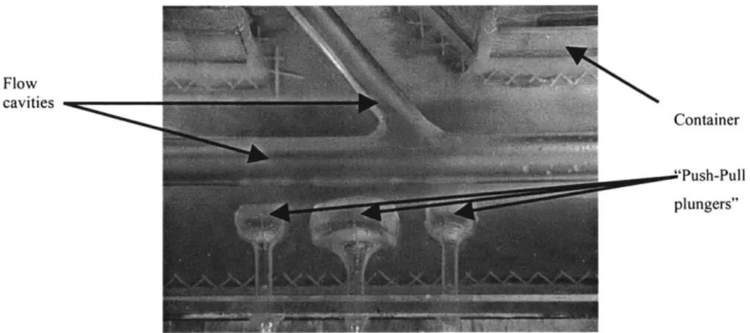
The flow model is formed in a Plexiglas container filled with a clear silicone compound,
into which cavities in the shape of different geometries in the arterial tree have been formed. Fluid is perfused through these cavities to simulate blood flow. Adjacent to these cavities are pneumatic spaces that can be inflated and deflated to compress adjacent flow channels. Silicon plungers function as pneumatic "pusher-pullers", so as to enable a dynamic alteration in flow channel geometry to simulate different disease states and/or clinical intervention schemes.
Flow cavities
Container
"Push-Pull plungers"
Figure 2-1: Flow model. Chamber, flow cavity and pneumatic "pusher-pullers" are indicated
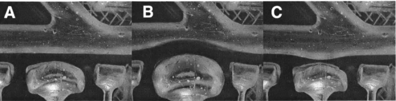
Figure 2-2: Operation of "push-pull plungers". (A) Device is deflated for normal geometry. (B) Device is pressurized to create lesion. (C) Vacuum is applied to create aneurysm.
The flow model is created in three main steps:
1. Creation of a solid cast of the flow channels and pneumatic spaces.
2. Fixation of solid cast in container and embedding in silicone.
3. Melting of the cast out of container to create flow channels/pneumatic spaces,
and connection to external flow/pressure channels.
I. 1 Creation of solid cast:
The material for the solid cast must be pliable enough to be shaped into smooth, non-obstructive flow models that are similar to arteries in their geometry and internal properties, and able to be melted out of the silicone without affecting its essential properties, such as optical clarity for flow imaging. Unfortunately, these properties are difficult to reconcile in one material. Initially wax was embedded directly into the
silicone and melted out. Unfortunately, the petroleum present in wax softens the wax and reacts with the silicone when heated causing it to become opaque. Thus, a staged process was used that included first formation of the initial cast from wax, then formation of a polyurethane mold and finally cast pouring.
I. .a. Formation of initial cast from wax: Sculptor's microcrystalline wax was used to create the cast as it is soft and pliable when heated, allowing molding into virtually any shape. When cooled, it becomes hard and smooth and the shape can be retained. Small pieces of the wax were heated to 75'C for approx. 4 minutes, and after slight cooling could then be rolled and kneaded into the required shapes. Bifurcations were formed by
joining two cylinders of wax and filling in the creases, and push-pull plungers were formed by connecting a small cylinder or hemi-cylinder to a long stem. Final shaping was performed when the wax had cooled completely to achieve as smooth a finish as possible.
Figure 2-3: Wax casts. Bifurcation model seen at top. Several push-pull plungers including concentric, one-sided and semi-circular are shown.
1.1 .b. Formation of polyurethane mold: Since wax cannot be melted out of the silicone
without altering its optical properties, and the PEG that is ultimately placed in the silicone can be poured but not shaped, a mold is required to transfer the cast from one material to the other. The material for formation of this mold was a two part polyurethane compound, Smooth-On PMC-121/30 Dry. The normal PMC-121/30 compound exudes a mold release material that dissolves the wax. A container for holding the wax and
polyurethane was assembled and sealed. The wax piece was suspended inside the container and aligned along a horizontal plane that passes through the entire wax piece. Long pieces were supported from below to prevent sagging.
String Support
Wax Plastelene
Container Support
Figure 2-4: Suspension of wax cast prior to polyurethane pouring
Polyurethane was mixed and poured into the container up to halfway up on the wax piece and then allowed to set partially. Plastic cylinders of approx. 1/2cm diameter and 6cm
would ultimately be used in aligning the two halves of the polyurethane mold. Once the bottom half of the mold was fully cured, a layer of Teflon spray, Smooth-On Mold Release, was sprayed on and allowed to dry. The second half of the polyurethane mold was poured into the container and allowed to cure. The mold was removed from the container, opened and the wax piece removed. The two halves were re-assembled using the plastic cylinders as guides for alignment.
1.1 .c. Pouring final cast: The final cast was made of Poly(Ethylene Glycol) (PEG). The
molecular weight of the PEG must be between 1000-1500 for the cast to be solid and smooth, but not brittle. The PEG was melted and poured into the polyurethane mold that had been placed vertically. Once the PEG cooled, the mold was opened and the PEG carefully removed.
The end properties of the PEG piece are highly sensitive to the temperature at which the melting was done. To produce a smooth non-brittle piece, the temperature cannot greatly exceed the melting temperature of the PEG. For the 1500 molecular weight PEG this should be no higher than 60'C.
1.2 Fixation of cast and embedding in silicone:
A clear Plexiglas container for the model was built and sealed using silicone
sealant. The bifurcation cast as well as all of the push-pull plungers were fixed in the container prior to embedding in the silicone of the final model. A gap of at least 3 cm between the container and outer most PEG piece prevented bursting of the model from imposed pressure. The PEG pieces were interfaced to the outside tubing through the container walls using specially built glass tubes. The details of the design (see fig. 2-5) of these tubes are crucial to their function.
15-20m
5/8T
23.9mm 8.5mm 1/4"7.5 _
2.5cm 1.Ocm 1.5cm
1.5" 3" 3.5"
Figure 2-5: Glass interface pieces. Left -example of interface piece for bifurcation arm with internal end (the end that stays inside container) facing right. Right - example of interface piece for pusher-puller with internal end facing left.
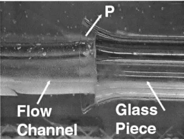
The inner diameter of the internal end was slightly oversized relative to the external diameter of the PEG piece. The flaring out of the internal end of both pieces creates an 0-ring effect that seals off the interface between the silicone cavity and the glass when the model is pressurized.
Figure 2-6: O-ring effect. In an image of the finished model, the top arrow indicates direction in which the pressure pushes the silicone on the inside of the glass interface to seal it against the flaring surface.
The mid portion of each glass tube was plugged by pouring molten PEG into it. The glass tube was then held vertically with the inner part facing up and the end of the PEG cast that was to interface with this piece inserted down to the plug. The narrow space between the PEG piece and the glass was sealed with molten PEG.
Figure 2-7: Interface sealing. One arm of PEG cast in glass tubing prior to sealing with molten PEG. PEG was poured into space indicated by arrow.
Holes were drilled in the walls of the Plexiglas container for the glass interface pieces. The interface pieces were threaded through the holes, sealed using silicone sealant and fixed in place with a ring of epoxy cement that surrounded the glass and bound it to the Plexiglas.
Figure 2-8: Fixation of PEG cast. Interface piece before (left) and after (right) fixation using epoxy ring.
If needed, push-pull plungers can be stabilized from above prior to pouring of bottom
half of silicone. After the bottom half has hardened and prior to pouring of top half, these supports can be removed as the pusher-pullers are now stabilized by the silicone.
GE Silicones RTV 6166 was mixed at a ratio of 1:2 part A to part B respectively rather
than the classic 1:1 ratio so as to increase the stiffness of the model. For models of depth greater than approx. 8cm it is preferable to pour the silicone in two halves; allowing the
bottom half to cure before pouring the top half. This two part process allows air bubbles to escape to the surface before the material is fully cured.
Figure 2-9: Model after curing of silicone. Bifurcation seen at top and three push-pull plungers for the main branch at the bottom.
1.3 Melting and connections:
The final step in fabrication of the flow model was melting the cast out of the silicone. The container with the silicone was mounted onto a wood backing and placed
vertically in an oven heated to 70*C. This temperature is sufficient to melt the PEG but
not high enough to warp the Plexiglas. Complete melting of the PEG takes overnight, and any residual PEG in the flow channels can be cleared by running hot water inside the model. Tubing from the pump was slid onto the external part of the glass interfaces.
Smaller diameter tubing was slid onto the external part of the interfaces for the push-pull plungers and then connected to syringes to impose the pressure differences that
inflate/deflate the plungers. The entire container was mounted to slope upwards from proximal to distal to ensure that no air bubbles would be trapped within the model
II. Instrumentation and analysis
I1.1 Flow circuit:
The flow circuit is comprised of all parts of the experimental flow apparatus other than the silicone model itself. This includes:
1. Lower reservoir and tubing - a container with a spout at the bottom. Filled with the perfusing fluid prior to running the model.
2. Pump - Harvard Apparatus Pulsatile Blood Pump model 1423. Provides independent control over stroke volume, frequency and systole/diastole ratio.
3. Proximal tubing and ports - 5/8" PVC tubing. Ports are glass connectors that allow access to the flow. These include: collateral take-off port, pressure-wire insertion port, proximal differential pressure sensor tubing port and particle injection port.
3.1. Collateral tube - 3/8" PVC tubing. The middle segment was made of silicone
tubing to allow flow constriction and modulation. This tube runs directly from the pump to the upper reservoir.
olla
erat
Particl~e
P
rt\Injection
Port
ressU re
e~[Pressure
.P rt
Wire Port
Figure 2-10: Proximal ports.
4. Flow model - described previously.
5. Distal tubing, ports and resistors - 5/8" PVC tubing leaves both branches of the model and was used to mount flow sensors. Distal to flow sensors, "/2" silicone tubing
on which resistors were mounted runs up to upper reservoir. Mother branch tubing can be fitted with pressure port for distal differential pressure sensor tubing in the same way as proximal port is done.
6. Upper reservoir and tubing - second container with spout at bottom and holes for insertion of distal tubing coming from model and collateral at top. The bottom spout was connected via tubing to top of lower reservoir.
Upper Reservoir
esispo
r
a
Collateral
11.2Flo wa efomaiston:Daughter
Vessel
Mothe
Vessel-Lower
Reservoir
Figure 2-11: Distal tubing and reservoirs.
Perfusing fluid: 40% aqueous glycerol solution with a measured kinematic viscosity of v = 0.027 Stokesn an a specific gravity of 1. 1.
II.2 Flow waveform acquisition:
Transonic C-series clamp-on ultrasonic sensors interfaced into a Transonic T-206 dual sensor controller unit were mounted on both the mother and daughter vessels and
flow-rate waveforms geneflow-rated. The sensors were located distal to the model on the tubing connected to each one of the two glass interface pieces.
These sensors provide two advantages: first, as they were not placed within the tubing they did not affect flow. Second, they measure the flow across the entire cross-section of the tube and hence are not affected by the shape of the flow profile. The output signal
from the Transonic systems controller was fed into an A/D board, National Instruments
DAQ-Pad 1200, working at bipolar (±5V) reference single ended mode. Data was
displayed and recorded using National Instruments LABView software at a sampling rate of 100Hz. The total flow in the collateral, where relevant, was determined from the
difference between the sum of the integrated flows in the two branches with the collateral open and when occluded. Since the pump characteristics remain the same, the difference was assumed to be the flow in the collateral.
Figure 2-12: Flow sensor. Image shows Transonic ultrasonic flow sensor mounted on tubing exiting model.
11.3 Pressure waveform acquisition:
Two options were available for generation of pressure waveforms: differential pressure between two locations and referenced pressure at a point.
II.3.A. Option A - Differential pressure:
A differential pressure sensor was fabricated using a Motorola MPX 1 ODP differential
pressure sensor (pressure range = 1-1.5 psi). For a description of the amplification circuits and operation see appendix A. Pressure input to this sensor is connected via two silicone tubes leading from the pressure tap in the flow tubing on one end, to the port on the differential pressure sensor on the other. The positive terminal on the sensor was connected to the proximal pressure tap and the negative terminal was connected to the distal pressure tap. The tubes themselves were air filled and thus avoided contact of fluid with sensor interior.
Figure 2-13: Differential pressure sensor.
II.3.B. Option B - Pressure at a point:
Another possibility for pressure measurement is to connect the proximal pressure tap to the positive terminal of the differential pressure sensor described above and leave the negative terminal open to air, or a hydrostatic column of fluid.
Figure 2-14: Proximal pressure measurement using differential pressure sensor.
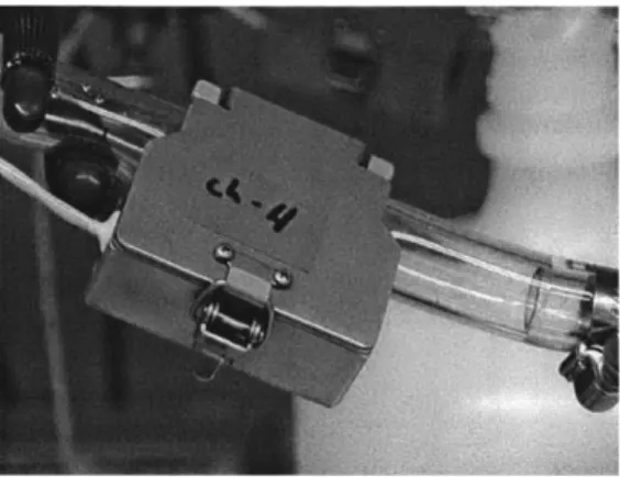
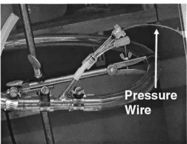
When pressure at an internal location was needed a pressure wire, RADI Medical PressureWire (RADI, Stockholm Sweden), was inserted via the pressure wire port and advanced to the point at which pressure was to be measured. The port opening was then sealed off.
Figure 2-15: Pressure wire insertion.
The RADI controller was fed into an amplification circuit (see appendix A) and the amplified signal was fed into the A/D board.
11.4 Waveform conditioning and synchronization
Once waveforms, pressure or flow, have been recorded they are loaded into MATLAB for analysis. Most of these waveforms are noisy and are digitally filtered (see appendix B) using a low-pass filter with a cutoff frequency of 1Hz. to preserve at least the first 10 harmonics of the fundamental frequency. For experiments that include both waveform and visualization (discussed in part III of this chapter), the waveform and video timeline must be synchronized. The method for synchronization is as follows:
1. At the end of the experiment the pump is turned off suddenly during mid systole.
2. Flow is allowed to subside for approx. 30 seconds and the pump is turned back on.
3. Steps 1&2 are repeated 3 or 4 times.
4. The instant at which the pump was turned off can be identified on the pressure waveform as a discontinuous fall in pressure. Similarly, the instant at which the pump was turned back on can be identified on the pressure waveform.
5. The same events as in step 4 can be identified on the video timeline by using Adobe Premiere to search for the loud clicking sound of the pump switch.
0.14 -- -- --- I 0.12 --- --- --- --- ---- -- --0.1 -0.06 - - - - - - -0.04 -0.02 --- - --- --- - --- --- - - --- - ----0 --- - - - -- --- --- ---
--0.02 --- --- --- --- --- --- r---r---I --- ---
I---0.04 - - - - - -- - - - - - -
--0.06 ---
----200 205 210 215 220 225 23) 235 240 245 lime feed,,
Figure 2-16: Waveform synchronization. Arrows indicate points on pressure waveform at which pump was turned off and then back on. Bottom panel shows audio file with sharp click sound caused by switch in middle.
6. The difference between these two timelines was averaged for several on/off
cycles and the waveform timeline was shifted accordingly so that both timelines coincide in time.
III. General flow visualization
Generation of flow visualization was performed in two parts. Enhanced still frames of the flow were produced and then reduced to quantifiable images. This section will describe the common process of generation of the still frames. Conversion of these frames to images of flow visualization will be described in the next chapter. Generation of still frames is comprised of three aspects:
1. Formation of tracer particles 2. Filming/image acquisition
3. Image enhancement.
111.1 Formation of Tracer particles:
Polymeric microspheres were custom-made to serve as tracer particles for the flow model. The technique employed allowed for control of particle size, buoyancy and color. The fabrication procedure is described below. Each batch of spheres produced approx. 800 microspheres of median size approx. 1.3mm, adequate for performing one stage of visualization.
1. Polymer solution: 4gr. Polymer mixture of poly(styrene) and poly(methyl methacrylate) at a mixture ratio of 7:3 respectively in 15cc Methylene Chloride. The ratio can be varied slightly in either direction to produce slightly heavier (less styrene) or lighter (more styrene) particles. The polymer was allowed to dissolve while stirring overnight.
2. Surfactant solution: 1% w/v poly(vinyl alcohol) in water. 300cc of this mixture is needed for one batch.
3. The surfactant solution was spun in a 500cc beaker using an overhead stirrer at a
rate of approx. 300 rpm.
4. The polymer solution was loaded into a Icc syringe and dropped at a rate that maintained individual drops into the spinning surfactant solution through a 26G needle. This was performed a total of 4 times.
5. The particles spun for 30 minutes and were then emptied into a second beaker spun with a stirrer bar overnight. Steps 4&5 were repeated until the entire 20cc of polymer mixture was consumed.