OSSOS. XII. Variability Studies of 65 Trans-Neptunian Objects Using the Hyper Suprime-Cam

(1)

HAL Id: hal-02372345

https://hal.archives-ouvertes.fr/hal-02372345

Submitted on 17 Dec 2020

HAL is a multi-disciplinary open access

archive for the deposit and dissemination of

sci-entific research documents, whether they are

pub-lished or not. The documents may come from

teaching and research institutions in France or

abroad, or from public or private research centers.

L’archive ouverte pluridisciplinaire HAL, est

destinée au dépôt et à la diffusion de documents

scientifiques de niveau recherche, publiés ou non,

émanant des établissements d’enseignement et de

recherche français ou étrangers, des laboratoires

publics ou privés.

Objects Using the Hyper Suprime-Cam

Mike Alexandersen, Susan Benecchi, Ying-Tung Chen, Marielle Eduardo,

Audrey Thirouin, Megan Schwamb, Matthew Lehner, Shiang-Yu Wang,

Michele Bannister, Brett Gladman, et al.

To cite this version:

Mike Alexandersen, Susan Benecchi, Ying-Tung Chen, Marielle Eduardo, Audrey Thirouin, et al..

OSSOS. XII. Variability Studies of 65 Trans-Neptunian Objects Using the Hyper Suprime-Cam.

As-trophysical Journal Supplement, American Astronomical Society, 2019, 244 (1), pp.19.

�10.3847/1538-4365/ab2fe4�. �hal-02372345�

(2)

DRAFT

Typeset using LA_{TEX default style in AASTeX62}

OSSOS XII: Variability studies of 65 Trans-Neptunian Objects using the Hyper Suprime-Cam

∗

M

IKE

A

LEXANDERSEN

,

1

_S

USAN

D. B

ENECCHI

,

2

_Y

ING

-T

UNG

C

HEN

,

1

_M

ARIELLE

R. E

DUARDO

,

3

_A

UDREY

T

HIROUIN

,

4

M

EGAN

E. S

CHWAMB

,

5

_M

ATTHEW

J. L

EHNER

,

1, 6, 7

_S

HIANG

-Y

U

W

ANG

,

1

_M

ICHELE

T. B

ANNISTER

,

8

_B

RETT

J. G

LADMAN

,

9

S

TEPHEN

D. J. G

WYN

,

10

_{JJ. K}

AVELAARS

,

10, 11

_J

EAN

-M

ARC

P

ETIT

,

12

AND

K

ATHRYN

V

OLK13

1_{Institute of Astronomy and Astrophysics, Academia Sinica; 11F of AS/NTU Astronomy-Mathematics Building, No. 1 Roosevelt Rd., Sec. 4, Taipei 10617, Taiwan} 2_{Planetary Science Institute, 1700 East Fort Lowell, Suite 106, Tucson, AZ 85719, USA}

3_{Department of Physical Sciences, University of the Philippines Baguio, Gov. Pack Rd., Baguio City, Benguet, Philippines 2600} 4_{Lowell Observatory, 1400 W Mars Hill Rd, Flagstaff, Arizona, 86001, USA}

5_{Gemini Observatory, Northern Operations Center, 670 North A’ohoku Place, Hilo, HI 96720, USA} 6_{Department of Physics and Astronomy, University of Pennsylvania, 209 S. 33rd St., Philadelphia, PA 19104, USA}

7_{Harvard-Smithsonian Center for Astrophysics, 60 Garden St., Cambridge, MA 02138, USA}

8_{Astrophysics Research Centre, School of Mathematics and Physics, Queen’s University Belfast, Belfast BT7 1NN, United Kingdom} 9_{Department of Physics and Astronomy, University of British Columbia, Vancouver, BC V6T 1Z1, Canada}

10_{Herzberg Astronomy and Astrophysics Research Centre, National Research Council of Canada, 5071 West Saanich Rd, Victoria, British Columbia V9E 2E7,}

Canada

11_{Department of Physics and Astronomy, University of Victoria, Elliott Building, 3800 Finnerty Rd, Victoria, BC V8P 5C2, Canada} 12_{Institut UTINAM UMR6213, CNRS, Univ. Bourgogne Franche-Comté, OSU Theta F25000 Besançon, France}

13_{Lunar and Planetary Laboratory, University of Arizona, 1629 E University Blvd, Tucson, AZ 85721, USA}

ABSTRACT

We present variability measurements and partial light curves of Trans-Neptunian Objects (TNOs) from a

two-night pilot study using Hyper Suprime-Cam (HSC) on the Subaru Telescope (Maunakea, Hawai’i, USA).

Subaru’s large aperture (8-m) and HSC’s large field of view (1.77 deg

2

_{) allow us to obtain measurements of}

multiple objects with a range of magnitudes in each telescope pointing. We observed 65 objects with m

r

= 22.6–

25.5 mag in just six pointings, allowing 20–24 visits of each pointing over the two nights. Our sample, all

discovered in the recent Outer Solar System Origins Survey (OSSOS), span absolute magnitudes H

r

= 6.2–

10.8 mag and thus investigates smaller objects than previous light curve projects have typically studied. Our

data supports the existence of a correlation between light curve amplitude and absolute magnitude seen in other

works, but does not support a correlation between amplitude and orbital inclination. Our sample includes a

number of objects from different dynamical populations within the trans-Neptunian region, but we do not find

any relationship between variability and dynamical class. We were only able to estimate periods for 12 objects

in the sample and found that a longer baseline of observations is required for reliable period analysis. We find

that 31 objects (just under half of our sample) have variability ∆

mag

greater than 0.4 mag during all of the

observations; in smaller 1.25 hr, 1.85 hr and 2.45 hr windows, the median ∆

mag

is 0.13, 0.16 and 0.19 mags,

respectively. The fact that variability on this scale is common for small TNOs has important implications for

discovery surveys (such as OSSOS or the Large Synoptic Survey Telescope) and color measurements.

Keywords:

Kuiper belt: general — minor planets, asteroids: general — planets and satellites: surfaces

1. INTRODUCTION

Over the years, rotational light curves (the brightness variation versus time) from small bodies in our Solar System have been

used to derive physical properties about the shape, surface, cohesion, internal structure, and density of objects, and to infer

binarity (

Sheppard et al. 2008

;

Thirouin et al. 2010

;

Benecchi & Sheppard 2013

). Small light curve amplitudes can be caused by

albedo variation across the surface of a spherical object, but moderate/large amplitude light curves (maximum minus minimum,

Corresponding author: Mike Alexandersen

mike.alexandersen@alumni.ubc.ca

∗_{Based on data collected at Subaru Telescope, which is operated by the National Astronomical Observatory of Japan.}

(3)

∆

mag

≥0.15-0.2 mag) are likely due to the shape of the object (

Sheppard et al. 2008

;

Thirouin et al. 2010

). Flat light curves

can be explained by a nearly-spherical object with a homogeneous surface or an elongated object with a pole-on orientation. A

flat light curve can also be due to an extremely slow rotational period undetectable during the observing window, and such a

slow rotation may infer the presence of a companion (

Thirouin et al. 2010

;

Benecchi & Sheppard 2013

;

Thirouin et al. 2014

).

Alternatively, very large amplitude light curves (∆

mag

≥0.9 mag) with a U-/V-shape at the maximum/minimum of brightness are

due to close/contact binary systems (

Sheppard & Jewitt 2004

;

Lacerda et al. 2014

;

Thirouin et al. 2017

;

Thirouin & Sheppard

2017

,

2018

;

Ryan et al. 2017

).

In the trans-Neptunian belt, four main dynamical populations - classical, resonant, detached and scattering objects - have

been identified with additional sub-divisions inside some of these broad groupings. Resonant objects are trapped in mean-motion

resonance with Neptune, such that the orbital period (or mean-motion) of the TNO and Neptune have a small integer ratio, which

causes the TNO to experience stabilizing gravitational perturbations. Objects that are currently interacting strongly with Neptune

in such a way that their orbits are unstable are called scattering (a semi-major axis change of at least 1.5 AU in 10 Myr is required

for this classification in the nomenclature of

Gladman et al. 2008

). The detached objects are those objects with perihelia that

are so distant that they are beyond significant gravitational influence from Neptune; how they got there is a subject of active

research. The resonant, detached and scattering objects are all dynamically excited (“hot”) populations, with wide inclination

and eccentricity distributions, thought to have been caused by significant interaction with the giant planets or other small bodies

during the era of planetary migration (

Kaula & Newman 1992

;

Malhotra 1993

,

1995

;

Thommes et al. 2002

;

Kortenkamp et al.

2004

;

Hahn & Malhotra 2005

;

Murray-Clay & Chiang 2005

;

Tsiganis et al. 2005

;

Levison et al. 2008

). The classical objects

consists of non-resonant, non-scattering objects, primarily located at semi-major axes between 42 AU and 48 AU. The classical

population has both a hot sub-population and a dynamically cold sub-population of object that have nearly circular orbits with

low inclinations and eccentricities; the dynamically cold objects likely had only limited interactions with the giant planets. Due

to their different formation mechanisms, it is possible that these dynamical populations have different light curve properties, just

as they have different color distributions (

Trujillo & Brown 2002

;

Peixinho et al. 2003

;

Fraser & Brown 2012

;

Sheppard 2012

;

Tegler et al. 2016

;

Pike et al. 2017

).

Because light curves of TNOs have been studied by several surveys over the past decades, it is now possible to study the

rotational properties of the different dynamical populations. Several studies have identified different correlations/anti-correlations

between orbital and physical/rotational properties, allowing us to understand the different dynamical environments in the

trans-Neptunian belt (

Duffard et al. 2009

;

Benecchi & Sheppard 2013

;

Thirouin et al. 2016

). However, most of the past surveys focused

on bright objects, as they are the easiest ones to study with small/moderate aperture facilities. Therefore, we present a pilot study

using the Subaru/HSC to study the rotational properties of the faint TNOs (H

r

> 8.0 mag). We aim to explore the rotational

properties of TNOs in several size ranges, particularly for smaller objects around the break in each population’s size distribution

(

Shankman et al. 2013

;

Fraser et al. 2014

;

Alexandersen et al. 2016

;

Lawler et al. 2018

); however, firm conclusions will require

additional observations.

2. SAMPLE & OBSERVATIONS

Our sample consists entirely of objects discovered or detected in the Outer Solar System Origins Survey (OSSOS,

Bannister

et al. 2016

,

2018

). OSSOS was a large program on the Canada-France-Hawaii Telescope (CFHT), which ran from 2013 through

2017. OSSOS detected and tracked more than 800 trans-Neptunian objects (TNOs) with regular follow-up observations during

at least two years to determine accurate orbits and secure dynamical classifications (

Bannister et al. 2018

). Due to the design and

success of OSSOS, we have very complete information on the orbital characteristics and classification of these objects. Likewise,

because these objects were discovered recently, they are still tightly clustered on the sky, having only slightly diffused apart due

to Kepler shear. This allows us to observe up to 17 objects at once within the 1.77 deg

2

field of view of Subaru Telescope’s Hyper

Suprime-Cam (HSC,

Miyazaki et al. 2018

). The six fields used in this study (coordinates in

Table 1

) were chosen in order to

maximize the number of objects within each field (see

Figure 1

), for a total of 63 TNOs (37 classical, 15 resonant, 5 detached,

6 scattering) and two Centaurs spanning apparent magnitudes m

r

= 22.6–25.5 mag and absolute magnitudes H

r

= 6.2–10.8 mag

(as calculated from our light curve observations). This sample far outnumbers (by a factor of 2.5) previously reported variability

studies for faint (H

r

≥ 8 mag) TNOs. Our sample thus much more thoroughly probes a smaller size regime than previous light

curve studies have typically studied, thanks to the combined aperture size and field of view of Subaru/HSC. Information about

the individual objects in our sample can be found in

Table 2

.

(4)

Table 1.

Field centers used in this work. On the second night, each field lost one or two

observations due to low transparency.

Field

Right Ascension

Declination

Observations night 1

Observations night 2

Identifier

(hrs)

(deg)

Useful/Total

LF07

00

h

31

m

33

s

+04

◦

54’54”

12/12

10/12

LF08

00

h

₄₁

m

₄₁

s

₊₀₅

◦

17’52”

12/12

10/12

LF09

00

h

42

m

34

s

+06

◦

37’44”

12/12

10/12

LF10

00

h

₄₅

m

₃₇

s

₊₀₇

◦

59’02”

12/12

10/12

LF11

01

h

10

m

00

s

+05

◦

43’25”

10/10

9/10

LF12

01

h

21

m

51

s

+06

◦

34’20”

10/10

9/10

6

8

10

12

14

16

18

20

22 RA (Degrees)

4

5

6

7

8

9 Dec (Degrees)

LF12

LF11

LF10

LF09

LF08

LF07

Figure 1. The location of our 2016 fields relative to TNOs discovered in the OSSOS L and S blocks (left and right, respectively). The large

field of view of HSC (magenta) allowed us to observe many objects at once. The field centers used are listed in

Table 1

.

Table 2. Summary of information about the objects in our sample. ID refers to the internal OSSOS designation (as used in (

Bannister

et al. 2018

)). Field is the field in which the target was observed (

Table 1

). a, e and i are the barycentric orbital parameters semi-major

axis, eccentricity and inclination (uncertainties on eccentricity and inclination are always 0.001 or smaller and are therefore not listed

here). Class is the dynamical classification of the object. MPC is the Minor Planet Center

2

designation (Note: all objects will have

MPC designations before final publication.). m

r

and H

r

are the mean apparent and absolute magnitudes of the objects, as measured

in this work (these are the magnitudes used everywhere in this paper, as they are more accurate than the discovery magnitudes from

OSSOS); due to the quality of the OSSOS orbits, the uncertainty on H

r

is identical to that of m

r

to the given precision. ∆

mag

is the

maximum magnitude variation measured for the object within this work. σ

mag

is the standard deviation of the magnitudes measured

in this work. This table is ordered in the same order as Figures

3 to

6 : brightest object at the top to faintest object at the bottom.

ID Field a(au) e i(deg) Class MPC mr(mag) Hr(mag) ∆mag σmag

o5t09PD LF09 67.760 ± 0.009 0.459 3.575 det 2014 UA225 22.627 ± 0.002 7.033 0.110+0.012−0.012 0.027 +0.002 −0.002 o3l43 LF11 45.785 ± 0.004 0.097 2.025 cla 2013 UL15 22.989 ± 0.002 6.702 0.363+0.012_−0.011 0.109+0.002_−0.002 o5s21 LF10 43.851 ± 0.007 0.170 2.373 cla 23.225 ± 0.003 7.564 0.36+0.02 −0.02 0.106 +0.003 −0.003 o3l57 LF12 45.044 ± 0.004 0.075 1.841 res 11:6 2013 UM15 23.297 ± 0.003 6.872 0.127+0.015_−0.014 0.034+0.003_−0.003 o5t03 LF09 25.967 ± 0.0014 0.288 18.849 cen 23.380 ± 0.003 10.825 0.15+0.03 −0.02 0.041 +0.004 −0.004

(5)

Table 2 (continued)

o5t34PD LF07 45.959 ± 0.003 0.170 5.081 res 17:9 2003 SP317 23.511 ± 0.006 7.226 0.56+0.05_−0.04 0.177+0.007_−0.006 o5s07 LF08 39.332 ± 0.004 0.249 16.270 res 3:2 23.615 ± 0.004 8.957 0.22+0.02 −0.02 0.048 +0.004 −0.003 o5s52 LF10 50.85 ± 0.03 0.247 27.196 res 11:5 23.616 ± 0.003 7.054 0.314+0.014 −0.014 0.094 +0.003 −0.003 o5s36 LF09 43.258 ± 0.003 0.053 2.206 cla 23.638 ± 0.003 7.569 0.43+0.02 −0.02 0.128 +0.004 −0.004 o5s05 LF10 21.981 ± 0.010 0.479 15.389 cen 2015 RV245 23.640 ± 0.004 10.767 0.10+0.02_−0.02 0.025+0.004_−0.004 o3l64 LF11 44.355 ± 0.003 0.073 1.972 cla 2013 UW16 23.729 ± 0.004 7.233 0.13+0.02_−0.02 0.038+0.004_−0.004 o3l46 LF12 46.612 ± 0.004 0.079 2.471 cla 2013 UP15 23.730 ± 0.004 7.404 0.29+0.02−0.02 0.089 +0.004 −0.004 o5t08 LF08 38.848 ± 0.003 0.057 1.097 cla 23.751 ± 0.004 8.164 0.21+0.02 −0.02 0.057 +0.004 −0.004 o5t30 LF08 43.791 ± 0.008 0.073 2.170 cla 23.811 ± 0.004 7.648 0.55+0.02 −0.02 0.159 +0.005 −0.005 o5t42 LF07 39.451 ± 0.011 0.204 1.587 res 3:2 23.833 ± 0.004 7.254 0.16+0.02 −0.02 0.045 +0.004 −0.004 o5s14 LF07 34.841 ± 0.002 0.047 7.122 res 5:4 23.911 ± 0.004 8.488 0.22+0.02 −0.02 0.054 +0.004 −0.004 o5t51 LF08 59.83 ± 0.10 0.425 13.851 res 14:5 23.936 ± 0.004 6.833 0.24+0.03 −0.02 0.057 +0.004 −0.004 o3l82 LF11 43.657 ± 0.005 0.286 24.987 res 7:4 2013 UK17 23.936 ± 0.005 6.621 0.15+0.02_−0.02 0.044+0.006_−0.005 o3l63 LF12 45.132 ± 0.004 0.054 3.363 cla 2013 UN15 23.986 ± 0.005 7.493 0.56+0.03_−0.03 0.161+0.005_−0.004 o3l83 LF11 200.2 ± 0.5 0.781 10.652 det 2013 UT15 24.001 ± 0.005 6.168 0.33+0.02_−0.02 0.098+0.005_−0.005 o5s35 LF09 46.40 ± 0.02 0.161 24.307 cla 24.065 ± 0.005 8.023 0.37+0.03 −0.03 0.106 +0.005 −0.005 o3l55 LF11 44.004 ± 0.004 0.096 2.358 cla 2013 UY16 24.086 ± 0.005 7.667 0.37+0.02_−0.02 0.121+0.005_−0.005 o5t16 LF08 44.79 ± 0.02 0.176 17.756 cla 24.158 ± 0.005 8.358 0.36+0.04 −0.03 0.093 +0.006 −0.006 o5s30 LF07 41.477 ± 0.005 0.073 33.327 cla 24.164 ± 0.007 8.247 0.27+0.03 −0.03 0.063 +0.006 −0.006 o3l71 LF12 45.319 ± 0.003 0.014 1.927 cla 2013 UW17 24.178 ± 0.006 7.612 0.42+0.03−0.03 0.125 +0.006 −0.005 o5t06 LF08 72.06 ± 0.03 0.535 12.327 sca 24.183 ± 0.006 8.941 0.25+0.03 −0.03 0.069 +0.006 −0.006 o5s22 LF10 46.162 ± 0.010 0.222 8.482 res 19:10 24.207 ± 0.005 8.538 0.21+0.02 −0.02 0.059 +0.005 −0.005 o5s15 LF07 45.439 ± 0.009 0.238 25.362 res 13:7 24.246 ± 0.006 8.809 0.31+0.03 −0.03 0.084 +0.006 −0.006 o3l65 LF11 44.609 ± 0.007 0.278 11.207 sca 2013 UZ16 24.272 ± 0.006 7.775 0.36+0.03_−0.03 0.095+0.007_−0.007 o3l20 LF12 39.425 ± 0.010 0.181 2.085 res 3:2 2013 UV17 24.335 ± 0.008 8.354 0.69+0.04_−0.04 0.185+0.008_−0.008 o5s19 LF10 45.054 ± 0.006 0.194 17.960 res 11:6 24.357 ± 0.006 8.758 0.38+0.03 −0.03 0.105 +0.006 −0.006 o5t10 LF07 37.844 ± 0.006 0.051 1.540 cla 24.375 ± 0.007 8.768 0.31+0.05 −0.04 0.081 +0.008 −0.008 o5t44 LF08 43.560 ± 0.004 0.071 3.566 cla 24.383 ± 0.007 7.768 0.28+0.03 −0.03 0.085 +0.005 −0.006 o3l62 LF11 39.230 ± 0.004 0.238 4.416 res 3:2 2013 UX16 24.415 ± 0.008 7.950 0.27+0.05−0.04 0.076 +0.010 −0.010 o5s24 LF10 50.376 ± 0.018 0.278 9.376 res 13:6 24.435 ± 0.007 8.657 0.58+0.04 −0.04 0.153 +0.007 −0.007 o3l19 LF11 45.334 ± 0.003 0.126 1.480 cla 2013 SM100 24.447 ± 0.007 8.507 0.68+0.04_−0.04 0.174+0.007_−0.007 o5s42 LF10 39.323 ± 0.011 0.165 5.772 res 3:2 24.482 ± 0.007 8.284 0.38+0.05 −0.04 0.102 +0.009 −0.010 o5t27 LF08 43.907 ± 0.011 0.079 1.498 cla 24.490 ± 0.007 8.348 0.42+0.04 −0.04 0.101 +0.006 −0.006 o5t48 LF07 42.183 ± 0.003 0.156 5.209 res 5:3 24.526 ± 0.011 7.693 0.41+0.04 −0.04 0.107 +0.009 −0.009 o5t13 LF08 79.06 ± 0.03 0.535 17.629 res 17:4 24.531 ± 0.007 8.849 0.41+0.05 −0.05 0.100 +0.008 −0.008 o5t32 LF08 43.791 ± 0.005 0.035 2.209 cla 24.537 ± 0.008 8.292 0.48+0.05 −0.05 0.117 +0.010 −0.010 uo3l84 LF11 44.012 ± 0.003 0.082 1.435 cla 24.547 ± 0.009 7.858 0.44+0.06 −0.06 0.117 +0.011 −0.010 o3l44 LF12 42.793 ± 0.005 0.042 2.940 cla 2013 UC18 24.557 ± 0.008 8.261 0.47+0.04_−0.04 0.141+0.010_−0.009 uo3l88 LF11 43.935 ± 0.004 0.081 2.479 cla 24.558 ± 0.007 8.275 0.53+0.04 −0.05 0.169 +0.009 −0.008 o5t07 LF07 39.513 ± 0.009 0.192 2.802 res 3:2 24.611 ± 0.014 9.159 0.48+0.06 −0.06 0.143 +0.015 −0.014 o5t41 LF08 44.310 ± 0.004 0.043 0.997 cla 24.659 ± 0.011 8.085 0.23+0.05 −0.04 0.068 +0.012 −0.009 o5t22 LF08 39.58 ± 0.02 0.176 5.457 res 3:2 24.664 ± 0.009 8.612 0.28+0.05 −0.03 0.076 +0.009 −0.008 o5t49 LF08 44.851 ± 0.004 0.096 1.968 cla 24.672 ± 0.008 7.807 0.64+0.04 −0.04 0.204 +0.008 −0.008 o5s61 LF10 44.942 ± 0.012 0.117 3.023 cla 24.696 ± 0.009 7.879 0.65+0.05 −0.04 0.177 +0.009 −0.009 o5t23 LF08 46.215 ± 0.007 0.132 5.089 cla 24.813 ± 0.009 8.760 0.66+0.08 −0.06 0.174 +0.012 −0.012 o5s40 LF09 44.310 ± 0.007 0.075 2.276 cla 24.965 ± 0.010 8.702 0.41+0.05 −0.04 0.117 +0.009 −0.009 o5t26 LF09 43.173 ± 0.004 0.043 16.024 cla 24.973 ± 0.013 8.855 0.41+0.07 −0.05 0.115 +0.014 −0.014

(6)

Table 2 (continued)

uo5t55 LF08 44.25 ± 0.02 0.073 1.544 cla 25.015 ± 0.011 8.702 0.54+0.08 −0.07 0.129 +0.013 −0.013 o5s29 LF07 41.396 ± 0.003 0.045 34.929 cla 25.023 ± 0.012 9.111 0.33+0.05 −0.04 0.097 +0.011 −0.011 o5s43 LF07 70.84 ± 0.07 0.465 10.192 det 25.044 ± 0.011 8.837 0.49+0.07 −0.08 0.120 +0.014 −0.015 o5t25 LF08 43.288 ± 0.006 0.047 0.461 cla 25.084 ± 0.012 8.971 0.40+0.06 −0.06 0.099 +0.011 −0.011 o5t21 LF08 43.633 ± 0.003 0.074 6.872 res 7:4 25.104 ± 0.014 9.082 0.59+0.07 −0.06 0.165 +0.013 −0.013 o5s55 LF09 46.93 ± 0.02 0.173 4.812 cla 25.107 ± 0.010 8.528 0.59+0.07 −0.06 0.148 +0.011 −0.010 o5s26 LF09 41.344 ± 0.007 0.112 17.483 cla 25.111 ± 0.014 9.299 0.54+0.05 −0.05 0.152 +0.012 −0.012 o5s12 LF10 34.791 ± 0.005 0.100 2.668 res 5:4 25.118 ± 0.015 9.798 0.40+0.08 −0.06 0.13 +0.02 −0.02 o5s49 LF07 44.017 ± 0.007 0.044 2.088 cla 25.178 ± 0.012 8.889 1.01+0.10 −0.09 0.22 +0.02 −0.02 o5s60 LF10 42.530 ± 0.007 0.128 40.362 cla 25.180 ± 0.012 8.510 0.51+0.07 −0.06 0.127 +0.012 −0.012 o5t24 LF09 44.953 ± 0.006 0.107 2.398 cla 25.257 ± 0.014 9.199 0.80+0.08 −0.08 0.20 +0.02 −0.02 o5s57 LF07 41.356 ± 0.011 0.140 32.358 cla 25.276 ± 0.016 8.649 0.84+0.10 −0.09 0.227 +0.016 −0.015 uo5s77 LF09 65.95 ± 0.11 0.413 38.607 res 13:4 25.604 ± 0.018 9.477 0.98+0.09 −0.09 0.295 +0.02 −0.02

Data were collected by M. Alexandersen and S.-Y. Wang on the nights of 2016 August 25 and 26, using HSC on Subaru

Telescope, located on Maunakea, Hawai’i, USA

3

_.

_{Figure 1}

_{shows our field locations in relation to the swarm of OSSOS TNOs.}

As TNOs are typically brightest in r-band, this filter was used. The six fields were observed in a repeated sequence with one

300 second exposure of each field, resulting in about 36 minutes between repeat observations of the same field. Because the

observing nights were approximately 1.5 months from opposition, we were unable to observe our fields for the entire night; the

four fields closer to opposition thus were observed 12 times each night, while two other fields were observed 10 times each night.

Observations were taken at airmasses ranging from 1.02 to 2.04. The conditions were generally good (transparency near 1.0,

seeing mostly between 0.65” and 1.0”), apart from about one hour of clouds and very low transparency on the second night. One

or two observations of each field were therefore unusable for this project.

3. PHOTOMETRY & CALIBRATION

Images were processed using hscPipe

4

, the official HSC data reduction software package, which includes calibration of

astrometry/photometry and basic image processing (bias, darks, and flats) (

Bosch et al. 2018

). hscPipe was developed as a

prototype pipeline for the Large Synoptic Survey Telescope (LSST) project (

Ivezic et al. 2008

). The algorithms and conceptions

of hscPipe were inherited from the Sloan Digital Sky Survey (SDSS) Photo Pipeline (

Lupton et al. 2001

). The standard outputs

of the hscPipe process include detection catalogs and calibrated images. We used the Pan-STARRS1 PV2 catalog (PS1,

Tonry

et al. 2012

;

Schlafly et al. 2012

;

Magnier et al. 2013

) as the reference catalog for photometry and astrometry.

Photometry of bright point sources revealed systematic variability (of order 0.01 magnitudes), caused by the fact that hscPipe

calibrates images individually; images of the same field can thus have slight discrepancies relative to each other due to

uncer-tainties in the zero-point determinations. To mitigate for this effect, background stars were inspected to find a set of 10-15

non-variable stars, defined as those that exhibit similar systematic variability, to reveal the systematic variability of the zero-point

error. A secondary correction was then applied to the zero points, such that the average magnitude of the non-variable stars is

constant across the set of images. This adjustment was typically smaller than 0.02 magnitudes, but is important for obtaining the

most accurate TNO photometry possible.

In order to get the best possible photometric measurements of our TNOs, we used the Python package TRIPPy (

Fraser et al.

2016

). TNOs move at typical rates of 3–6”/hr at opposition, thus moving up to 0.5” during our 300-second exposures, causing

slight trailing. TRIPPy uses knowledge of the rate and angle of motion to accurately measure photometry for moving objects

using an elongated aperture and appropriate aperture correction.

We obtained 9–23 useful measurements for each object over two nights; the median number of measurements per object is 19.

One or two images per field were discarded due to low transparency during one hour on the second night; while some reduced

transparency can be corrected for in calibration, we found that images with transparency < 50% consistently produced anomalous

results, so we chose to exclude those images. Many objects lost one or more measurement due to being too close to a background

source for reliable photometry. Three objects (o5t41, o5t07 and o5s12) only have data on one night because they fell into chip

3_{All data obtained as part of this project can be downloaded from https://smoka.nao.ac.jp/fssearch or http://www.cadc-ccda.hia-iha.nrc-cnrc.gc.ca/en/search/} 4_{https://hscdata.mtk.nao.ac.jp:4443/hsc_bin_dist/index.html}

(7)

gaps on one of the two nights; this was difficult to avoid when optimizing field location for up to 17 objects moving at different

rates. One object (o5t44) was on a different chip on the two nights; however, we are confident that our zero point calibration is

accurate such that there is not an offset between the two nights. The final calibrated photometric measurements as well as the

calibrated zero points can be found in

Table 3

.

[tbp]

Table 3. Photometric measurements from this HSC data

set. σ

Rand

is the random uncertainty of the m

r

magnitude

measurement. Z p is the zero-point used. σ

Sys

is the

sys-tematic uncertainty on the zero-point (and thus also on the

measurement). This is an example for a single object; all

measurements from all 65 objects are available in machine

readable format in the on-line supplements.

MJD−57620

m

r

± σ

Rand

Z p

± σ

Sys

o3l19

6.3913125

24.09 ± 0.03

26.995 ± 0.005

6.4154337

24.21 ± 0.02

27.012 ± 0.005

6.4393438

24.45 ± 0.02

27.022 ± 0.005

6.4634385

24.69 ± 0.04

27.058 ± 0.005

6.4876346

24.78 ± 0.03

27.047 ± 0.005

6.5123402

24.56 ± 0.03

27.039 ± 0.005

6.5375195

24.41 ± 0.03

27.043 ± 0.005

6.5628085

24.29 ± 0.03

27.045 ± 0.005

6.5875091

24.28 ± 0.02

27.038 ± 0.005

7.3876072

24.55 ± 0.03

26.978 ± 0.005

7.4114040

24.67 ± 0.03

27.002 ± 0.005

7.4353624

24.45 ± 0.02

26.885 ± 0.005

7.4595078

24.47 ± 0.02

26.869 ± 0.005

7.5081300

24.36 ± 0.03

26.497 ± 0.005

7.5584662

24.35 ± 0.02

27.019 ± 0.005

7.5830743

24.42 ± 0.02

27.004 ± 0.005

7.6079518

24.58 ± 0.02

26.994 ± 0.005

4. RESULTS

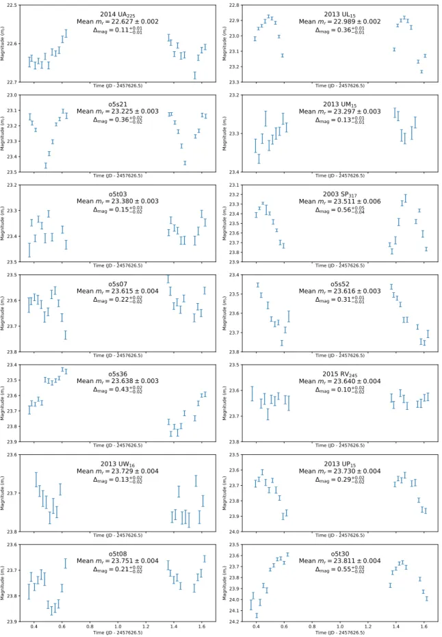
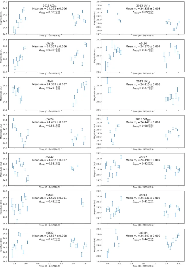
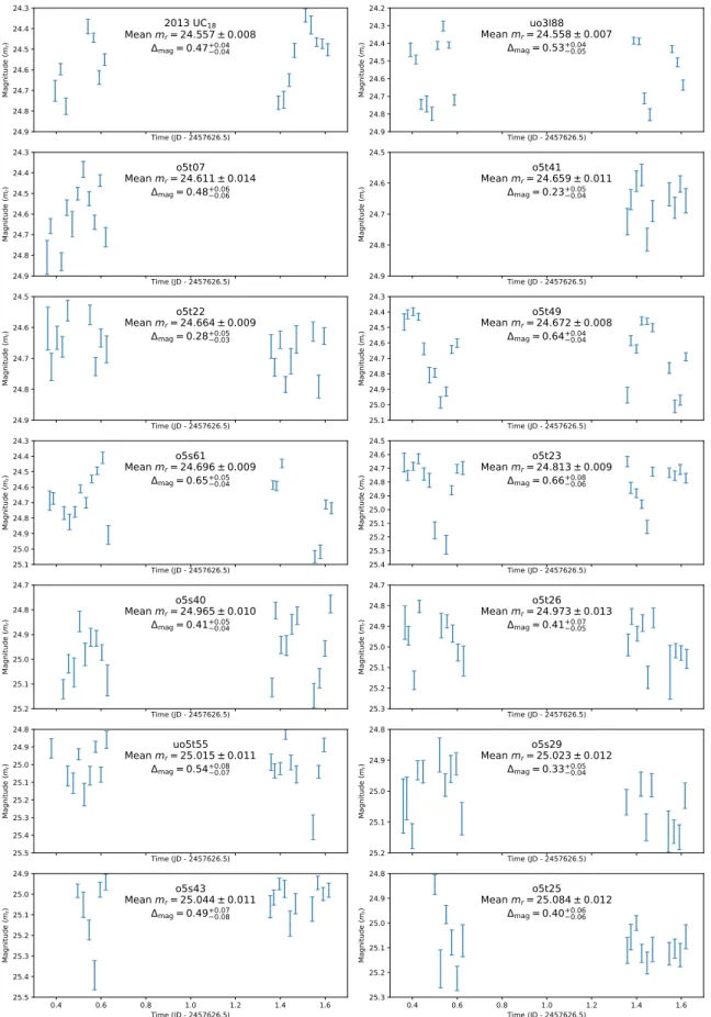
We have measured partial light curves for 63 TNOs and two Centaurs. The measurements can be found in graphical form in

Figures

2 to

6 ; the photometric data can be found in

Table 3

. Several objects (such as 2013 UL

15

, o5s21, 2003 SP

317

, o5t30 and

2013 UN

15

) feature clear, high-amplitude variability. We have investigated the relationships between our measured light curve

variability and other properties such as absolute magnitude, dynamical class, and other orbital parameters (

Section 4.1

). For the

best quality light curves, estimates of the rotation periods were also made (

Section 4.2

).

In order to estimate the uncertainty on parameters such as the magnitude variation, period, correlation coefficient and so on,

a resampling method was used. One thousand resampled datasets were generated by resampling each magnitude measurement

of each object. This resampling was drawn from a normal distribution centered on the measured value with a width equal to the

measurement uncertainty. The analysis was then performed on each resampled dataset independently to find the distribution of

(8)

Time (JD - 2457626.5) 22.5 22.6 22.7 Ma gn itu de (mr )

2014 UA

225

Mean m

r

= 22.627 ± 0.002

mag

= 0.11

+0.010.01 Time (JD - 2457626.5) 22.8 22.9 23.0 23.1 23.2 23.3 Ma gn itu de (mr )

2013 UL

15

Mean m

r

= 22.989 ± 0.002

mag

= 0.36

o5s21

Mean m

r

= 23.225 ± 0.003

mag

= 0.36

+0.020.02 Time (JD - 2457626.5) 23.2 23.3 23.4 Ma gn itu de (mr )

2013 UM

15

Mean m

r

= 23.297 ± 0.003

mag

= 0.13

+0.010.01 Time (JD - 2457626.5) 23.2 23.3 23.4 23.5 Ma gn itu de (mr )

o5t03

Mean m

r

= 23.380 ± 0.003

mag

= 0.15

+0.030.02 Time (JD - 2457626.5) 23.1 23.2 23.3 23.4 23.5 23.6 23.7 23.8 23.9 Ma gn itu de (mr )

2003 SP

317

Mean m

r

= 23.511 ± 0.006

mag

= 0.56

o5s07

Mean m

r

= 23.615 ± 0.004

mag

= 0.22

+0.020.02 Time (JD - 2457626.5) 23.4 23.5 23.6 23.7 23.8 Ma gn itu de (mr )

o5s52

Mean m

r

= 23.616 ± 0.003

mag

= 0.31

o5s36

Mean m

r

= 23.638 ± 0.003

mag

= 0.43

2015 RV

245

Mean m

r

= 23.640 ± 0.004

mag

= 0.10

+0.020.02 Time (JD - 2457626.5) 23.6 23.7 23.8 Ma gn itu de (mr )

2013 UW

16

Mean m

r

= 23.729 ± 0.004

mag

= 0.13

2013 UP

15

Mean m

r

= 23.730 ± 0.004

mag

= 0.29

+0.020.02 0.4 0.6 0.8 1.0 1.2 1.4 1.6 Time (JD - 2457626.5) 23.6 23.7 23.8 23.9 Ma gn itu de (mr )

o5t08

Mean m

r

= 23.751 ± 0.004

mag

= 0.21

+0.020.02 0.4 0.6 0.8 1.0 1.2 1.4 1.6 Time (JD - 2457626.5) 23.5 23.6 23.7 23.8 23.9 24.0 24.1 24.2 Ma gn itu de (mr )

o5t30

Mean m

r

= 23.811 ± 0.004

mag

= 0.55

+0.020.02

(9)

Time (JD - 2457626.5) 23.7 23.8 23.9 24.0 Ma gn itu de (mr )

o5t42

Mean m

r

= 23.833 ± 0.004

mag

= 0.16

o5s14

Mean m

r

= 23.911 ± 0.004

mag

= 0.22

o5t51

Mean m

r

= 23.936 ± 0.004

mag

= 0.24

2013 UK

17

Mean m

r

= 23.936 ± 0.005

mag

= 0.15

+0.020.02 Time (JD - 2457626.5) 23.6 23.7 23.8 23.9 24.0 24.1 24.2 24.3 Ma gn itu de (mr )

2013 UN

15

Mean m

r

= 23.986 ± 0.005

mag

= 0.56

2013 UT

15

Mean m

r

= 24.001 ± 0.005

mag

= 0.33

o5s35

Mean m

r

= 24.065 ± 0.005

mag

= 0.37

2013 UY

16

Mean m

r

= 24.086 ± 0.005

mag

= 0.37

o5t16

Mean m

r

= 24.158 ± 0.005

mag

= 0.36

o5s30

Mean m

r

= 24.164 ± 0.007

mag

= 0.27

2013 UW

17

Mean m

r

= 24.178 ± 0.006

mag

= 0.42

o5t06

Mean m

r

= 24.183 ± 0.006

mag

= 0.25

+0.030.03 0.4 0.6 0.8 1.0 1.2 1.4 1.6 Time (JD - 2457626.5) 24.0 24.1 24.2 24.3 24.4 Ma gn itu de (mr )

o5s22

Mean m

r

= 24.207 ± 0.005

mag

= 0.21

+0.020.02 0.4 0.6 0.8 1.0 1.2 1.4 1.6 Time (JD - 2457626.5) 24.0 24.1 24.2 24.3 24.4 Ma gn itu de (mr )

o5s15

Mean m

r

= 24.246 ± 0.006

mag

= 0.31

+0.030.03

(10)

Time (JD - 2457626.5) 24.0 24.1 24.2 24.3 24.4 24.5 Ma gn itu de (mr )

2013 UZ

16

Mean m

r

= 24.272 ± 0.006

mag

= 0.36

+0.030.03 Time (JD - 2457626.5) 23.8 23.9 24.0 24.1 24.2 24.3 24.4 24.5 24.6 24.7 Ma gn itu de (mr )

2013 UV

17

Mean m

r

= 24.335 ± 0.008

mag

= 0.69

o5s19

Mean m

r

= 24.357 ± 0.006

mag

= 0.38

o5t10

Mean m

r

= 24.375 ± 0.007

mag

= 0.31

o5t44

Mean m

r

= 24.383 ± 0.007

mag

= 0.28

2013 UX

16

Mean m

r

= 24.415 ± 0.008

mag

= 0.27

o5s24

Mean m

r

= 24.435 ± 0.007

mag

= 0.58

2013 SM

100

Mean m

r

= 24.447 ± 0.007

mag

= 0.68

+0.040.04 Time (JD - 2457626.5) 24.2 24.3 24.4 24.5 24.6 24.7 24.8 Ma gn itu de (mr )

o5s42

Mean m

r

= 24.482 ± 0.007

mag

= 0.38

o5t27

Mean m

r

= 24.490 ± 0.007

mag

= 0.42

o5t48

Mean m

r

= 24.526 ± 0.011

mag

= 0.41

o5t13

Mean m

r

= 24.531 ± 0.007

mag

= 0.41

+0.050.05 0.4 0.6 0.8 1.0 1.2 1.4 1.6 Time (JD - 2457626.5) 24.2 24.3 24.4 24.5 24.6 24.7 24.8 24.9 Ma gn itu de (mr )

o5t32

Mean m

r

= 24.537 ± 0.008

mag

= 0.48

+0.050.05 0.4 0.6 0.8 1.0 1.2 1.4 1.6 Time (JD - 2457626.5) 24.3 24.4 24.5 24.6 24.7 24.8 24.9 Ma gn itu de (mr )

uo3l84

Mean m

r

= 24.547 ± 0.009

mag

= 0.44

+0.060.06

(11)

Time (JD - 2457626.5) 24.3 24.4 24.5 24.6 24.7 24.8 24.9 Ma gn itu de (mr )

2013 UC

18

Mean m

r

= 24.557 ± 0.008

mag

= 0.47

uo3l88

Mean m

r

= 24.558 ± 0.007

mag

= 0.53

o5t07

Mean m

r

= 24.611 ± 0.014

mag

= 0.48

o5t41

Mean m

r

= 24.659 ± 0.011

mag

= 0.23

o5t22

Mean m

r

= 24.664 ± 0.009

mag

= 0.28

o5t49

Mean m

r

= 24.672 ± 0.008

mag

= 0.64

o5s61

Mean m

r

= 24.696 ± 0.009

mag

= 0.65

o5t23

Mean m

r

= 24.813 ± 0.009

mag

= 0.66

o5s40

Mean m

r

= 24.965 ± 0.010

mag

= 0.41

o5t26

Mean m

r

= 24.973 ± 0.013

mag

= 0.41

uo5t55

Mean m

r

= 25.015 ± 0.011

mag

= 0.54

o5s29

Mean m

r

= 25.023 ± 0.012

mag

= 0.33

+0.050.04 0.4 0.6 0.8 1.0 1.2 1.4 1.6 Time (JD - 2457626.5) 24.9 25.0 25.1 25.2 25.3 25.4 25.5 Ma gn itu de (mr )

o5s43

Mean m

r

= 25.044 ± 0.011

mag

= 0.49

+0.070.08 0.4 0.6 0.8 1.0 1.2 1.4 1.6 Time (JD - 2457626.5) 24.8 24.9 25.0 25.1 25.2 25.3 Ma gn itu de (mr )

o5t25

Mean m

r

= 25.084 ± 0.012

mag

= 0.40

+0.060.06

(12)

Time (JD - 2457626.5) 24.7 24.8 24.9 25.0 25.1 25.2 25.3 25.4 25.5 Ma gn itu de (mr )

o5t21

Mean m

r

= 25.104 ± 0.014

mag

= 0.59

o5s55

Mean m

r

= 25.107 ± 0.010

mag

= 0.59

o5s26

Mean m

r

= 25.111 ± 0.014

mag

= 0.54

o5s12

Mean m

r

= 25.118 ± 0.015

mag

= 0.40

+0.080.06 Time (JD - 2457626.5) 24.7 24.8 24.9 25.0 25.1 25.2 25.3 25.4 25.5 25.6 25.7 25.8 25.9 26.0 Ma gn itu de (mr )

o5s49

Mean m

r

= 25.178 ± 0.012

mag

= 1.01

o5s60

Mean m

r

= 25.180 ± 0.012

mag

= 0.51

+0.070.06 Time (JD - 2457626.5) 24.8 24.9 25.0 25.1 25.2 25.3 25.4 25.5 25.6 25.7 25.8 Ma gn itu de (mr )

o5t24

Mean m

r

= 25.257 ± 0.014

mag

= 0.80

+0.080.08 0.4 0.6 0.8 1.0 1.2 1.4 1.6 Time (JD - 2457626.5) 24.7 24.8 24.9 25.0 25.1 25.2 25.3 25.4 25.5 25.6 25.7 25.8 Ma gn itu de (mr )

o5s57

Mean m

r

= 25.276 ± 0.016

mag

= 0.84

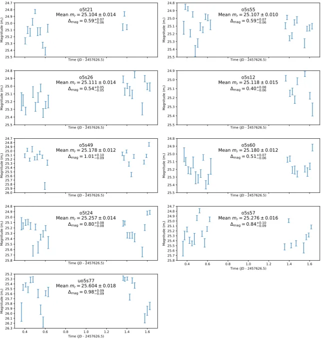
+0.100.09 0.4 0.6 0.8 1.0 1.2 1.4 1.6 Time (JD - 2457626.5) 25.2 25.3 25.4 25.5 25.6 25.7 25.8 25.9 26.0 26.1 26.2 26.3 Ma gn itu de (mr )

uo5s77

Mean m

r

= 25.604 ± 0.018

mag

= 0.98

+0.090.09

Figure 6. Absolutely calibrated photometry of our TNO sample. Objects 56–64, ordered by average magnitude.

resultant values. The 2σ uncertainty on a value is then taken to be the range that spans the central 95% of values (ie. 2.5% in

each tail).

4.1. Amplitude analysis

The mean rotational period of TNOs has been found to be 7–9 hours (

Duffard et al. 2009

;

Benecchi & Sheppard 2013

;

Thirouin

et al. 2016

), although periods range from 3.9 hours (Haumea) to 154 hours (Pluto). While we don’t have full light curves for all

of our target objects, the mean period of 7–9 hours means that we likely observed a near-maximum and near-minimum of most

of our target objects. Simple simulations of our observations confirm that for objects of a given period between 3 and 40 hours,

we observe more than 80% of the variability on average (averaged over random starting phase); for periods between 3 and 22

hours, we observe more than 88% of the variability on average. It is thus reasonable to assume that our measurements of ∆

mag

(maximum minus minimum magnitude) are close to the full light curve amplitudes and that the slight underestimation will not

affect our results (such as whether or not correlations exist). In this subsection, we have removed the two Centaurs (2015 RV

245

and o5t03) from the sample, because the surface and rotation of these objects might have been altered by close approaches to the

(13)

6

7

8

9

10 H

r

(m

ag

)

40

50

60

70

80 a (

AU

)

0

5

10

15

20 # of TNOs

0

10

20

30

40 i (

de

g)

0.0

0.2

0.4

0.6

0.8

1.0 mag

(mag)

0

5

10 # of TNOs

0.00 0.05 0.10 0.15 0.20 0.25 0.30

mag

(mag)

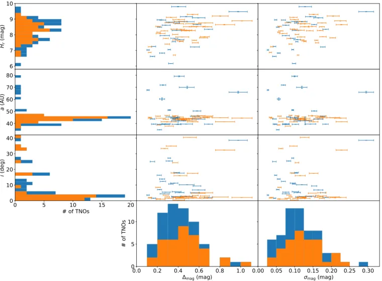
Figure 7. Left and bottom sides: histograms of H

r

magnitude, semi-major axis a, inclination i, ∆

mag

and σ

mag

of our data. Center and top right:

scatter plots of these parameters. Classical TNOs are shown in orange, and non-classical objects are shown in blue.

Sun or planets (

Thirouin et al. 2010

;

Duffard et al. 2009

). As an alternative to the difference between the brightest and faintest

observation (∆

mag

), we also examine the standard deviation (σ

mag

) of all the observations of each object, because the standard

deviation is a measure of overall variation that is less influenced by individual anomalous measurements.

In

Figure 7

, we plot both ∆

mag

and σ

mag

versus object H

r

, semi-major axis a, and inclination i to illustrate possible relations

between these parameters. In a sample of 128 objects,

Benecchi & Sheppard

(

2013

) found a statistically significant correlation

(ρ = 0.288, P = 0.001) between light curve amplitude and absolute magnitude. Their sample spanned absolute magnitudes from

0 to 12 mag, although most were between 4 and 7 mag; very few had absolute magnitude fainter than 8 mag. Our sample of 63

TNOs span H

r

= 6.2–10.8 mag

5

, with more than half the sample at H

r

> 8.0 mag; our sample thus represents variability properties

for fainter TNOs than the bulk of the

Benecchi & Sheppard

(

2013

) sample. Using the Spearman Rank correlation test (

Spearman

1904

) and our independent sample of 63 TNOs, we find ρ = 0.37, P = 0.003 for ∆

mag

versus H

r

and ρ = 0.31, P = 0.013 for

σ

mag

versus H

r

. Our data thus strongly support the existence of a weak relationship where intrinsically fainter (likely smaller)

bodies on average have larger light curve amplitudes. This is likely due to increasingly elongated shapes.

Benecchi & Sheppard

(

2013

) also found a borderline significant anti-correlation (ρ = −0.170, P = 0.056) between light curve amplitude and inclination

(i), however, our data do not support the existence of such an anti-correlation.

Because the cold classicals are thought to have formed in place while all the hot populations (hot classicals, resonant, detached

and scattering) are thought to have been scattered outwards to some extent after having formed closer to the Sun (e.g.

Li et al.

5_{Whenever we discuss apparent and absolute magnitudes for our sample objects, those magnitudes are measured/calculated from our light curves observations,}

(14)

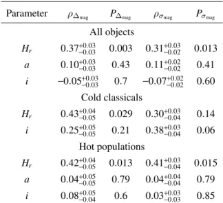
Table 4.

Spearman Rank correlation test results. Tests for

correlation between the measured light curve variation ∆

mag

and σ

mag

and the parameter listed in the first column.

Parameter

ρ

∆mag

P

∆mag

ρ

σmag

P

σmag

All objects

H

r

0.37

+0.03_−0.03

0.003

0.31

+0.03_−0.02

0.013 a

0.10

+0.03 −0.03

0.43

0.11

+0.02 −0.02

0.41 i

−0.05

+0.03_−0.03

0.7 −0.07

+0.02_−0.02

0.60 Cold classicals

H

r

0.43

+0.04−0.05

0.029

0.30

+0.03 −0.04

0.14 i

0.25

+0.05 −0.05

0.21

0.38

+0.03 −0.04

0.06 Hot populations

H

r

0.42

+0.04_−0.05

0.013

0.41

+0.03_−0.04

0.015 a

0.04

+0.05 −0.05

0.79

0.04

+0.04 −0.04

0.79 i

0.08

+0.05 −0.04

0.6

0.03

+0.03 −0.03

0.85 2008

;

Levison et al. 2008

;

Batygin et al. 2011

), we also test the dynamically cold and hot samples separately to identify whether

a trend might be present in one population and not in the other. In this work, we use the term “hot population” to refer to all of

the dynamically excited populations combined (as done in

Fraser et al. 2014

, and others); specifically our hot population sample

contains everything non-classical plus classical objects with i ≥ 6

◦

. Our “cold classicals” sample consists only of classicals with

i

≤ 4

◦

_{. Classicals with 4}

◦

_{< i < 6}

◦

_{(two objects in our sample) are excluded from either sample to minimize contamination.}

The correlation values as well as their significance levels can be found in

Table 4

and are simply summarized here. For our

samples of 26 cold classical TNOs and 35 hot TNOs, we find that both have similar correlation coefficients to the full sample for

amplitude versus H

r

, but with a lower significance than in the full sample (likely due mostly to the now smaller sample sizes).

For amplitude versus inclination, we find that neither population has a statistically significant correlation, just as in the overall

sample. Because the semi-major axis (a) is possibly related to where objects formed, we also tested for correlations between

the light curve variation and a for the full sample and the hot population (the cold population was not tested due to its narrow a

range). We find that the semi-major axis is not at all correlated with the variability in the full sample nor in the hot population.

To further test the notion that different populations may have different amplitude distributions, the 2-sample Anderson-Darling

test was used to compare subsamples. The subsamples used were the classical, resonant, hot and cold populations. We did not

look at the scattering and detached objects in this analysis because the sample sizes are too small for any meaningful results. In

every case, the subsample was tested against the remainder of the sample (ie. classicals versus everything non-classical, etc). See

Table 5

for the resultant P values. No subsample was found to be significantly different from the rest of the sample.

4.2. Period analysis

The rotation periods of TNOs range from 3.9 hours (Haumea) to 154 hours (Pluto), with a mean of 7–9 hours (

Duffard et al.

2009

;

Benecchi & Sheppard 2013

;

Thirouin et al. 2016

); there are clearly a number of assumptions and biases that go into

this mean, not the least of which is the aliasing effects from observations on consecutive nights and the fact that tracking low

amplitude and slowly varying objects requires a lot of telescope time. Both of these biases exist in our dataset; nevertheless, we

seek to use the data we present here to at least place limits on the rotation periods and amplitudes of the objects in our sample.

In the few cases where our data allow for more extensive interpretation, we proceed as appropriate for each object. We attempt

to fit periods to our light curve data using two methods: a Phase Dispersion Minimization (PDM) method and a Power Spectral

Density (PSD) method. Because our TNOs are all small enough that we do not expect them to be spherical, they should all

have double peaked periods. The two light curve peaks of an elongated TNO are often difficult to distinguish (for a perfectly

symmetrical ellipsoid, the two peaks would be identical). These methods therefore simply identify the period of the light curve,

(15)

Table 5.

2-sample Anderson-Darling test results.

Tests for whether two samples are likely to have been

drawn from the same source population. Here we test

whether the light curve variability (measured by ∆

mag

and σ

mag

) distribution is different for different

dynam-ical sub-populations. In every case here, a sub-sample

is tested against the remainder of our sample (eg. the

resonant objects against everything that is not

reso-nant).

sub-population

N

obj

P

∆mag

P

σmag

classicals

37

0.15

+0.10 −0.07

0.11

+0.06 −0.05

resonant

15 0.8 ± 0.2

0.76

+0.12 −0.14

hot

35

0.13

+0.09 −0.06

0.09

+0.06 −0.03

cold

26 0.4 ± 0.2

0.29

+0.12 −0.09

not the TNO. We double the single-peaked periods found by our two period methods to get the most likely rotation period of the

TNO.

Because our observing window is about 30 hours (from the start of night one to the end of night two) we are able to sample

rotation periods from the rotational break-up-limit of 3.3 hours (

Romanishin & Tegler 1999

) to about 60 hours (where we are

sampling half a rotation, which is a full peak-to-peak cycle for a double-peaked light curve). For the PSD method, we therefore

fold the light curves using every period from 1.0 hours to 30.0 hours in 0.1 hour intervals. The Fourier coefficients are calculated

from each folded light curve; the sum of the squares of the Fourier coefficients as a function of period is the PSD. The period that

has the highest PSD value is selected as the most likely period of the TNO. In the PDM method, we fit the data points for each

object using a modified PDM (

Stellingwerf 1978

;

Buie et al. 2018

). This method goes through every possible period, folds the

data and fits a second-order Fourier series to each folded light curve. The quality of each fit is captured from the residuals; the

fits are ranked and the fit with the highest quality is selected.

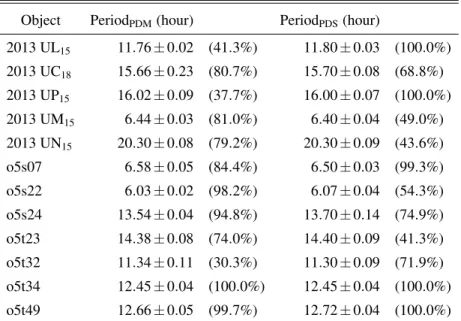
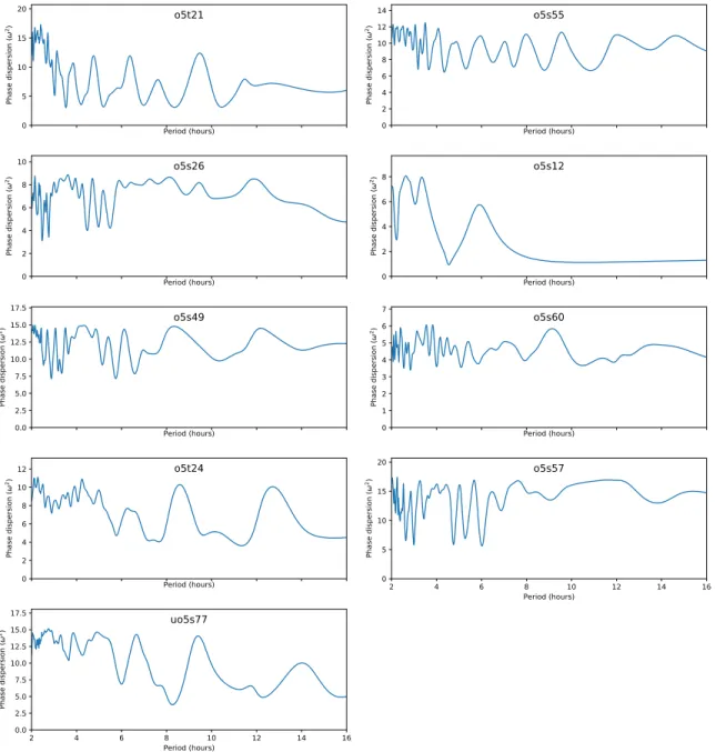
Table 6

lists the periods found from these two methods (converted into double-peak periods) for objects where the two methods

agree;

Figure 8

shows the light curves folded at those periods. When the two methods do not agree, it is likely evidence that

we do not have enough data to determine the period with confidence. The PDM curves from our period analysis is available in

the supplementary materials, Figures

10 to

14 . Although the mean period from our dataset analysis is somewhat greater than

that given in the literature (∼ 12.3 hours compared with 7-9 hours,

Duffard et al.

(

2009

);

Benecchi & Sheppard

(

2013

);

Thirouin

et al.

(

2010

)) it is important to recognize that the periods we are reporting are based on single epoch measurements without the

same fidelity of many of the light curves in the literature. The literature contains both single and double-peaked light curves and

light curves of binary objects. We cannot distinguish among these interpretations and have assumed a double-peaked light curve

for all objects, so one should not over-interpret this apparent result from our dataset. This sample of 12 periods is insufficient to

draw any conclusions, other than the fact that we would need a larger baseline than two consecutive 6-hour nights to determine

the period of a larger fraction of objects. Adding a third night and observing closer to opposition (when the targets are visible

for 8 hours) would allow determination of periods for a much larger fraction of light curves. We therefore leave discussion of the

period distribution for future work.

5. DISCUSSION AND CONCLUSIONS

5.1. Implications for large surveys

Large variability can have an influence on whether or not an object is discovered in a magnitude limited survey. Most large

surveys use an automated moving object pipeline to find TNO candidates. For the Canada-France Ecliptic Plane Survey (

Kave-laars et al. 2009

;

Petit et al. 2011

), OSSOS and the

Alexandersen et al.

(

2016

) survey, TNOs were identified using three discovery

images with one hour between each. Non-stationary sources within three images of a field are linked together as a candidate TNO

detection; various constraints on the rate, angle and linearity of motion are imposed, as well as a requirement of similar

magni-tudes, in order to limit the number of false candidates. If a TNO’s magnitude is highly variable, this might leave it undetected,

(16)

23.3

23.2

23.1

23.0

22.9

22.8 Ma

gn

itu

de

m

r

2013 UL

15 Period = 11.78 hr

24.4

24.3

24.2

24.1

24.0 o5s22

Period = 6.05 hr

23.4

23.3

23.2 2013 UM

15 Period = 6.42 hr

24.8

24.7

24.6

24.5

24.4

24.3

24.2

24.1

24.0 o5s24

Period = 13.62 hr

23.9

23.8

23.7

23.6

23.5

23.4

23.3

23.2

23.1 Ma

gn

itu

de

m

r

2003 SP

317 Period = 12.45 hr

24.9

24.8

24.7

24.6

24.5

24.4

24.3

24.2 o5t32

Period = 11.32 hr

23.8

23.7

23.6

23.5

23.4 o5s07

Period = 6.54 hr

24.9

24.8

24.7

24.6

24.5

24.4

24.3

24.2 2013 UC

18 Period = 15.68 hr

24.0

23.9

23.8

23.7

23.6

23.5 Ma

gn

itu

de

m

r

2013 UP

15 Period = 16.01 hr

25.1

25.0

24.9

24.8

24.7

24.6

24.5

24.4

24.3 o5t49

Period = 12.69 hr

0.0

0.2

0.4

0.6

0.8

1.0 Phase

24.4

24.3

24.2

24.1

24.0

23.9

23.8

23.7

23.6 2013 UN

15 Period = 20.30 hr

0.0

0.2

0.4

0.6

0.8

1.0 Phase

25.4

25.3

25.2

25.1

25.0

24.9

24.8

24.7

24.6

24.5 o5t23

Period = 14.39 hr

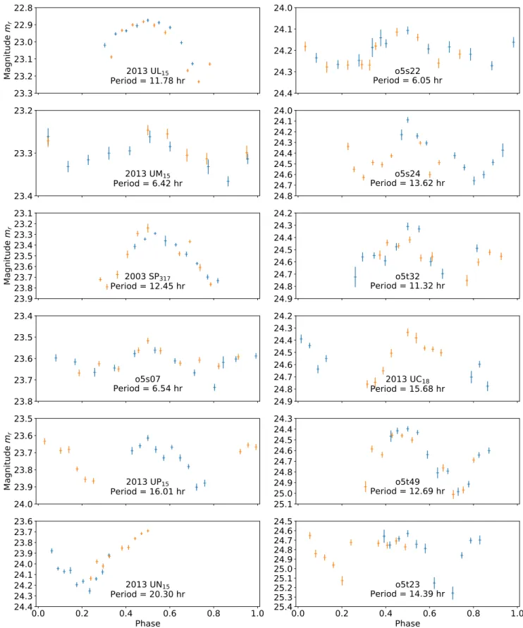
Figure 8. Folded light curves for the 12 objects for which we have a period estimate. Blue and orange points show data from the first and

second nights, respectively. The arbitrary phase=0 point was chosen such that the brightest measured magnitude falls at phase=0.5. The exact

values of MJD, magnitude and uncertainty of all observations can be found in

Table 3

.

(17)

Table 6. Best periods from two methods, in hours. Numbers in parentheses are the

percentage of resampled light curves that had a “best” period within 5σ of the reported

value. Only objects where the two methods agree on the best period are included. As

these objects are small, their variability is most likely shape-dominated; shape

domi-nated light curves have two peaks per rotation of the object.

Object

Period

PDM

(hour)

Period

PDS

(hour)

2013 UL

15

11.76 ± 0.02

(41.3%)

11.80 ± 0.03

(100.0%)

2013 UC

18

15.66 ± 0.23

(80.7%)

15.70 ± 0.08

(68.8%)

2013 UP

15

16.02 ± 0.09

(37.7%)

16.00 ± 0.07

(100.0%)

2013 UM

15

6.44 ± 0.03

(81.0%)

6.40 ± 0.04

(49.0%)

2013 UN

15

20.30 ± 0.08

(79.2%)

20.30 ± 0.09

(43.6%)

o5s07

6.58 ± 0.05

(84.4%)

6.50 ± 0.03

(99.3%)

o5s22

6.03 ± 0.02

(98.2%)

6.07 ± 0.04

(54.3%)

o5s24

13.54 ± 0.04

(94.8%)

13.70 ± 0.14

(74.9%)

o5t23

14.38 ± 0.08

(74.0%)

14.40 ± 0.09

(41.3%)

o5t32

11.34 ± 0.11

(30.3%)

11.30 ± 0.09

(71.9%)

o5t34

12.45 ± 0.04

(100.0%)

12.45 ± 0.04

(100.0%)

o5t49

12.66 ± 0.05

(99.7%)

12.72 ± 0.04

(100.0%)

either because it might be too faint to be detected in one of the three images or, if the constraints in the detection pipeline are too

tight, because the pipeline might not consider the three points to be the same object due to having different magnitudes.

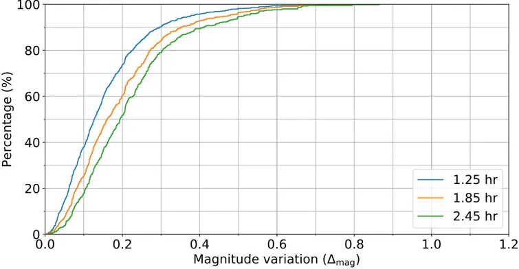
In our sample of 63 TNO light curves (most having observation on both nights), we find that only 6 ± 1 have a ∆

mag

< 0.2

magnitudes, while 31 ± 2 (just under half the sample) have a ∆

mag

> 0.4 magnitudes and 11 ± 1 have ∆

mag

> 0.6 magnitudes

6

.

However, those variations are usually over many hours. In order to evaluate the impact that light curve variation could have

on shorter timescales, we measured the typical variation on 1–2 hour timescales. Since our images for these light curves are

typically spaced 36 minutes apart, we calculated the ∆

mag

for all 1.25 hr (3 images), 1.85 hr (4 images) and 2.45 hr (5 images)

subsets of our light curves. We find that in 1.25 hr, the median value of the ∆

mag

is 0.13 magnitudes and the standard deviation

of the ∆

mag

distribution is 0.12 magnitudes. For 1.85 hr, the median and standard deviation are 0.16 and 0.13, respectively, while

for 2.45 hr they are 0.19 and 0.14 magnitudes, respectively.

Figure 9

shows the ∆

mag

distribution within these three time spans.

The moving object pipeline used for the

Alexandersen et al.

(

2016

) survey and for OSSOS only had the weak constraint that the

faintest and brightest points within the three discovery images (spaced about 1 hour apart) had to have a flux-ratio of less than

4, which corresponds to a magnitude difference of about 1.5 mag. In our data from this work, we never see variability greater

than 1.2 mag within a 2-hour window; it therefore seems highly unlikely that a real objects was rejected by the detection pipeline

due to natural variability. Because the overall average variability seen within our data is much larger than the average variability

measured within 1.25-2.45 hours, this demonstrates the perhaps obvious point that the average magnitude measured within a few

hours is not an accurate measurement of the true average magnitude of the TNO. Discovery images from surveys like CFEPS,

OSSOS and the

Alexandersen et al.

(

2016

) survey all depend on having measured the magnitude in three discovery images; the

fact that these measured magnitudes are potentially several tenths of a magnitude from the true average magnitude should be

included when performing survey simulation and model analysis.

Variability is important to consider when measuring photometric colors of TNOs as well. Because most facilities do not have

the ability to observe in multiple band-passes simultaneously, the images in different filters must be taken in sequence. If the

object is faint and thus requires a long exposure time in some/each filter, its variability could cause an erroneous measurement

of the color if the brightness varies significantly within the timespan of the observations. For accurate photometric colors, it

6_{The uncertainties quoted in this sentence on the number of objects come from resampling the light curve photometry 1000 times and calculating the values}

(18)

0.0

0.2

0.4

0.6

0.8

1.0

1.2 Magnitude variation (

mag

)

0

20

40

60

80

100 Percentage (%)

1.25 hr

1.85 hr

2.45 hr

Figure 9. Cumulative distribution of the magnitude variation (maximum minus minimum, ∆

mag

) within 1.25 hr (blue, top), 1.85 hr (orange,

middle) and 2.45 hr (green, bottom) sections of light curves.

is therefore important to account for light curve variability, except in cases of very short (thus nearly simultaneous) exposure

sequences for bright objects. This can be done by repeating observations of the filter that requires least exposure time several

times during a sequence (for example r-g-r-J-r), as has become common practice, to get a rough idea of the light curve variation

during the sequence. Alternatively, if some of the filters require enough exposure time to warrant multiple exposures, those

exposures should be spread out in the sequence (for example the r-g-J-g-r sequence used by

Bannister et al.

(

2017

)). Of course,

this relies on having fast filter changes and can therefore not be done with Hyper Suprime-Cam, which has a filter exchange time

of about 30 minutes. It should be obvious that photometry acquired on different days cannot be used to calculate reliable colors

unless the light curve is known, so TNO colors reported from surveys like the Hyper Suprime-Cam Subaru Strategic Program

(HSC SSP

Aihara et al. 2018

;

Terai et al. 2018

) or the LSST survey should be seen as very rough color estimates with a likely

uncertainty of ∼ 0.2 magnitude.

Expected to start science operations in 2022, LSST will provide an inventory of the trans-Neptunian region down to a 5-σ

limiting magnitude of approximately 24.6 in r and 24.8 in g (

Ivezic et al. 2008

;

LSST Science Collaboration et al. 2009

). LSST

is expected to discover over 40,000 TNOs during its planned ten years of science operations (

LSST Science Collaboration et al.

2009

). During this period, TNOs within the survey footprint will be imaged hundreds of times by LSST in multiple filters

(ugrizy), producing sparsely sampled light curves. Our HSC variability study overlaps the size and magnitude range that LSST

will be sensitive to. Thus, the variability we observe can be taken as a minimum value for the variability LSST will see for

its TNO sample. Over a few hour baseline, 90% of our HSC sample vary in brightness up to 0.4 magnitudes. This is more

variability than shallower past wide-field Solar System surveys had to deal with. As detailed above, OSSOS, which our sample is

derived from, had no significant brightness/variability constraints when identifying moving objects (

Bannister et al. 2018

). This

may be important in the development of the LSST moving object detection pipeline and for consideration when assessing the

TNO detection completeness for LSST. Additionally, in the sparse light curves LSST will produce, objects with more than 0.5

magnitudes variation can potentially be flagged as extreme shapes in need of further higher-cadence follow-up observations.

Finally, we note that objects in this size range do not have enough mass to ensure hydrostatic equilibrium, so the variability seen

is therefore most likely caused by the objects being highly non-spherical. Given the correlation between absolute H

r

magnitude

and variability shown above, it is unreasonable to expect that even smaller object can be modeled as roughly spherical shapes.

A number of surveys have searched for serendipitous stellar occultations by small (diameters ∼1 km, roughly corresponding

to H

r