Effect of Geometry Under Emitter Membrane on Pressure
Compensating Performance
by Tristan McLaurin MASSACHUSETTS IN'STITUTE OF TECHNOLOGY JLBR162019LIBRARIES
Submitted to the
ARCHIVES
Department of Mechanical Engineering
In Partial Fulfillment of the Requirements for the Degree of
Course 2-A: Bachelor of Science in Engineering as Recommended by the Department of Mechanical Engineering
at the
Massachusetts Institute of Technology
June 2019
Tristan McLaurin. All rights Reserved.
The author hereby grants to MIT permission to reproduce and to distribute publicly paper and electronic copies of this thesis document in whole or in part in any medium now
known or hereafter created.
Signature of Author:
Certified by:
Signature redacted
Department of Mechanical Engineering May 23, 2019
Signature redacted
m s G. Winter Associate Professor of M Engineering Thesis Advisor
Signature redacted
Accepted by:
Maria Yang Professor of Mechanical Engineering Undergraduate Officer
Effect of Geometry Under Emitter Membrane on Pressure
Compensating Performance
By
Tristan McLaurin
Submitted to the Department of Mechanical Engineering On May 11, 2019 in Partial Fulfillment of the
Requirements for the Degree of
Course 2-A: Bachelor of Science in Engineering as Recommended by the Department of Mechanical Engineering
Abstract
In order to better understand pressure compensating drip irrigation emitters, an experiment was carried out in order to characterize the effects of emitter dimensions under the membrane on emitter performance. Emitter performance was characterized by two models, an overdamped model and a piecewise model. A comparison of the models found an overdamped model to predict parameters with a greater degree of certainty than the piecewise model. No trends in emitter behavior could be identified with 95% certainty,
but slight trends were noted for their ability to possibly inform future emitter design.
Thesis Supervisor: Amos Winter Title: Associate Professor
Parameters and Variables used in this Thesis
* a or A are the first parameter of the overdamped model * b or B are the second parameter of the overdamped model * c or C are the third parameter of the overdamped model * i is the first parameter of the piecewise model
* j
is the second parameter of the piecewise model * k is the third parameter of the piecewise model* X is space between the outlet hole of an emitter and the center of the chamber under the membrane in the square chamber tests, as shown in figure 6
* Y is the depth of the chamber beneath the membrane in a prototype emitter in the square chamber tests, as shown in figure 6
* W is the distance between the outlet hole of an emitter and the center of the chamber under the membrane in the sinusoidal chamber tests, as shown in figure 24.
* Z is the depth of the chamber beneath the membrane in a prototype emitter in the sinusoidal chamber tests, as shown in figure 24.
* Q
is the flow rate of water across a given cross sectional area * P is pressureP
PA is the activation pressure of the emitter
* H is the Heaviside step function
* P is the pressure of the water entering the emitter * p is the density of the water
* Q
is the flow rate of the water leaving the emitter* PA is the activation pressure of the emitter * fD is the darcy friction factor
* L is the length of the pipe in which flow is taking place
* Dh is the hydraulic diameter * v is the mean flow velocity
* V is viscosity
* g is the acceleration due to gravity
* A is the cross-sectional area water is moving through * p is the wetted perimeter of the water passes around
I 1 is the length of a square pipe cross section * w is the width of a square pipe cross section
* Kpath loss is a parameter summarizing the minor losses due to the tortuous path
* Kchamber loss is a parameter summarizing the friction losses in the chamber under
the membrane
2 Introduction
Drip irrigation is an irrigation process where water is directly dripped over plants at a controlled rate. There are several benefits to drip irrigation as a method of irrigating crops. By dripping water at a controlled rate directly to the plants that need it rather than spraying it over a field, drip irrigation wastes less water by reducing evaporation and percolation below the root zone. Experimental results have indicated that drip irrigation also saves 40-80% more water than other irrigation methods [1]. Furthermore, drip irrigation has been shown to yield between 25%-60% more crop output than furrow irrigation [2]. Not only does drip irrigation waste less water and produce more crop yields, but it is also more profitable. The total revenue from drip irrigation systems are between 167%-400% greater than competing irrigation systems [2]. This means that farmers using drip systems can and do use less water, get higher crop yields, and receive greater incomes than farmers using other drip systems. However, there are still barriers to farmers
adopting drip systems. Two major barriers are capital cost of the system and clogging of drip emitters by particles in water, which leads to high maintenance requirements from the farm staff [3]. A better understanding of what influences emitter behavior can help address both of these issues. In order to better understand the behavior of drip irrigation emitters, an experiment was carried out to characterize the effect of an emitter's geometry on its behavior.
3 Background/Theory 3.1 Physical Meaning of Terms
Pressure compensating drip emitters are designed to emit water at a specified flow rate after reaching a required activation pressure. The behavior of once such emitter was recorded in an experiment by. Dr Charles M. Burt [4] (Fig. 1).
10
@00* 0 * * * . . 0
4 - - Manufacturer's Published
Nominal Flow Rate
2 -.. Experimental Data
0
I I I0 0.5 1 1.5 2 2.5 3
Pressure (bar)
Figure 1: Experimental results from a Netafim emitter's performance Note that the manufacturer's published flow rate is lower than the average flow rate, and that there is a
slight dip in flow rate after the emitter "activates" around 0.75 bar [4].
While manufacturers publish activation pressures and nominal flow rates for their emitters, the meaning of these terms are unclear. For example, one set of Netafim emitters consistently emitted water above the manufacturer's published flow rate. For some
emitters, the flow rates for emitters after their "activation" were not always constant, instead still showing a positive or negative trend [4]. Characterizing these traits is of
interest to us, as emitters with lower activation pressure can be used in systems with lower power and energy requirements and lower initial capital costs [3]. It is also useful to
a field at differing distances from their water source emit the same flow rate. This is characterized by how much the flow rate of an emitter varies after it has activated. This is because in a field, emitters farther from a water source will experience greater pressure drops and so be operating at a different pressure than emitters closer to the water source [7]. If an emitter has low uniformity, emitters closer to a pump may have a significantly different flow rate than that of emitters farther from a pump, which can waste water or fail to provide crops with the water they need [8]. As such, it is necessary to develop models defining the activation pressure and uniformity of an emitter.
3.2 Overdamped Model
The overdamped system model is used when modeling a system whose
performance experiences feedback. It is commonly used to model second order control systems, such as RLC circuits. An overdamped system has several features which resemble the performance of an emitter. It increases in value rapidly, before reaching a constant slope [5]. This behavior can be seen in figure 2.
0 c. C 7
Ii
7
7 6. 6- 6 0@0V~
V
144 4 0 0.5 1 15 0 0.5 1 1.5 2 0 0.5 1 1.5 2Pressure [Bar] Pressure [Bar Pressure (Bar]
Figure 2: The performance of several emitter prototypes developed in the writing of this paper. Note that they rapidly reach a high pressure then continue to act at a constant slope,
rather than achieving a constant flow rate after which the emitter performance does not change. The red data points refer to experimental data collected, while the cyan line refers
The second order system which would govern the behavior of an overdamped system would be found as follows:
0 = C + + C3 (1.0)
C _C__
Q (P) = K1 -e cl + K2 C3p (1.1)
C2 C2
Constraining this equation to a flow rate of zero when the pressure entering the emitter is zero so that Q(P=O) =0 indicates that equation 1.1 can be simplified as follows:
A = K1-E = K2 (1.2) C2 B = C2 (1.2) C, C = C3 (1.3) C2 Q(P) = AeBP A + CP (1.4)
where P refers to the pressure of the water entering the emitter and Q refers to the flow rate of water leaving the emitter. The three parameters A, B, and C can, therefore, be used to characterize a continuous model of emitter behavior. In this case, the activation pressure can be characterized using parameter B. As can be seen from equation 1.4, so long as
parameter B is negative, as the pressure increases the effect of the exponential part of the model decreases after which point the model becomes more linear. Therefore, this paper will define the activation pressure as the point where the exponential part of the equation contributes a magnitude of only 5% of A to the performance of the emitter:
where PA is the activation pressure of the emitter. This also means that the parameter C can be used to characterize the uniformity of the emitter, with a more uniform emitter having a value of C close to zero.
3.3 Piecewise Model
A physical model of the performance of the emitter can be constructed by
comparing the performance of the emitter to the pressure losses we expect it to experience. There are three pressure losses we expect to be significant in the emitter. A loss due to the water flowing through the tortuous path, a loss due to the flow through the chamber under the membrane, and a loss due to the water passing from a channel with the diameter of the chamber under the membrane to a diameter of the outlet hole.
The pressure loss due to the tortuous path is a loss due to the water moving through bends, and the pressure loss due to the water passing from a channel with the diameter of the chamber under the membrane to a diameter of the outlet hole is a sudden contraction. Both behaviors can be described as minor pressure losses within the emitter. Minor losses can be used to describe a relationship between pressure and flow rate as follows:
Kminor loss = P [6] (2.00) 2 P = Kminor loss 1 pV2 (2.01) = Kminor loss1 p(Q )2 (2.02) Q2 = 2A2p (2.03) Kminor lossP
Q
= 2Ap (2.04) Kminor lossPBy grouping all unknowns other than the pressure, we can say that the effect of the tortuous path on flow based on pressure is:
Q
= Kpath lossvpf (2.05)While the effect of the change in diameter as water through the outlet is:
Q
= Koutiet lossVf (2.06)The pressure loss occurring in the chamber under the membrane can be
represented using the Darcy-Weisbach equation. The Darcy-Weisbach equation relates head loss due to friction in a pipe to the average velocity of the fluid flow for an
incompressible liquid, and is written as follows:
= fD [6] (2.07)
where fD is the Darcy friction factor, L is the length of the pipe in which flow is taking place,
Dh is the hydraulic diameter, v is the mean flow velocity, p is the density of the fluid, and g
is the acceleration due to gravity. Rewriting this equation so that flow rate is written in terms of pressure: p(Q2) P = fDL 2 2AzDh (2.08) PfD L 2 (2.09)
Q
2 = p 2ADh (2.10) fDLBy grouping all unknowns other than the pressure, we can say that the effect of the chamber under the membrane is:
Q
= Kchamber loss (2.12)Note that all of these elements describing the behavior of
Q
has a factor of-'if.
Based on this relation, we would expect the relationship between the flow rate of the emitter and the pressure entering the emitter as:Q
= (Kpath loss + Kchamber loss + Koutiet loss)'fThis can be simplified by rewriting all unknown parameters in the equation so:
(2.13)
Q
=i'
(2.14)In the piecewise model, we expect that before the emitter reaches activation pressure, this pressure loss coefficient i is nearly constant and depends solely on the geometry of the emitter. Above activation pressure, the emitter's membrane deforms in
such a way as to increase the friction loss coefficient and alter the relationship between
Q
and P. If the emitter is compensating in an ideal way,Q
should become independent of P above activation pressure, which means that i needs to be linearly proportional to P. Thus we can construct a piecewise model for emitters based on the performance of the emitterhaving two regimes: a regime before the emitter has "activated," where it is experiencing losses similar to those experienced by the a minor friction loss, and a regime after it has been activated, where the emitter flow rate has a constant slope. The equation for this model can be written as:
Q(P)
=[iVif
x H(PA - P)] + [(jP + k) x H(P - PA)] (2.15)where H is the Heaviside step function, P is the pressure of the water entering the emitter,
emitter. In this case, parameters i, j, and k can be used to characterize the model, and the activation pressure PA can be found by:
jPA+k (2.16)
(2.17) = 2
i-4i 2jk-2]k 2j2
4 Experimental Design
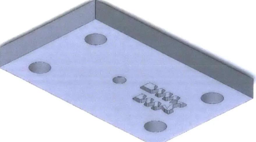
In order to test the effects of emitter geometry on performance, prototype emitters were machined out of aluminum to match the features which would be in an injection-molded plastic emitter if it were manufactured according to industry practices. The flow of water through the aluminum emitters is the same as what would be seen in a plastic
emitter (Fig. 2). Water from inlets flows over the top of a silicone membrane, through a tortuous path, and into a rectangular chamber, which is covered by the bottom of the silicone membrane. Water is then released through an outlet hole at the bottom of the rectangular chamber. The open areas of the emitter plate, other than the inlet and outlet, are covered and sealed by a top plate and a bottom plate clamped together.
Figure 2: Side view of water flow through an emitter prototype. Water flows over the membrane (1) through a tortuous path (not shown) and down through a hole (2) leading to a passage (3) which brings the water to a rectangular chamber under the membrane (4).
Water is then released through an outlet hole (5). The open areas which must be covered by the top and bottom plates are areas (2) and (3).
The top plate has the tortuous path and an inlet through which water from the pump enters the emitter (Fig. 3). Machining the tortuous path in the top plate allowed for a shorter machining time for each emitter prototype, and maintained a consistent tortuous path resistance between prototypes, while features under the membrane were altered. This allowed the experiments to isolate the effects of the geometry below the membrane on emitter behavior.
4,
'1'~*~
Figure 3: The top plate of the emitter prototype assembly. The tortuous path is machined into the top plate, and there is an inlet hole for water to be pumped into the emitter.
The full emitter assembly can be seen in Figure 4.
(a) (b)
Figure 4: Exploded view of a top plate, emitter, and bottom plate used in testing, as viewed from (a) above the assembly, (b) below the assembly. The emitters used in testing were changed while the same top and bottom plates were used for each test. The plates
were clamped together by screws placed in the corner holes, tightened with the same torque.
The experiment was conducted by pumping water with a SHURFLO 4008-101-E65 3.0 Revolution water pump through the emitter at a controlled pressure. A series of valves were used to control the pressure, and a Dwyer DPGW-07 Digital Pressure gauge with 1% accuracy was used to read the pressure entering the emitter. The water released from the emitter was collected for one minute, then the volume was measured in a graduated
cylinder in order to determine the emitter's flow rate at this pressure. Emitters were tested at pressures ranging from 0 to 2 Bar. This experimental setup can be seen in Figure 5.
Air -ReleaseEmte ValvePrtyp Pressure !Wow- am 5 GaugeEmte .. Volumetric WlowRar uMeasurement ve a) b)
Figure 5: a) Photograph of the experimental test setup with labels for each element of the setup. b) Flow chart indicating the water flow path in the experimental setup. Tests were conducted comparing the performance of emitters by varying two dimensions, both in the chamber under the membrane (area (4) in figure 2): the distance of the outlet hole from the center of the chamber under the membrane (parameter X in Figure 6) and the depth of the surface the inlet and outlet holes are drilled into below the bottom of an undeformed membrane (parameter Y in Figure 6).
A
Y
A
SECTION A-A
Figure 6: The two dimensions varied in the experiments. The dimension X is the distance between the emitter outlet hole and the center of the chamber under the membrane. The dimension Y is the depth of the surface the outlet hole is drilled into beneath the bottom of
the membrane.
The parameters used in the seventeen emitters tested are detailed in table 1.
X=0.00 mm NA NA NA
Y=0.25mm
X=0.00 mm X=2.30 mm X=3.30 m X=4.30 mm
Y=0.50 mm Y=0.50 mm Y=0.50 mm Y=0.50 mm
X=0.00 mm NA NA NA
Y=0.75 mm.
X=0.00 mm X=2.30 mm X=3.30 m X=4.30 mm
Y=1.00 mm Y=1.00 mm Y=1.00 mm Y=1.00 mm
X=0.00 mm X=2.30 mm X=3.30 m X=4.30 mm
Y=1.50 mm Y=1.50 mm Y=1.50 mm Y=1.50 mm
Table 1: X and Y values used for the 14 emitters tested.
We expect dimension Y to have an effect on the flow of the water due to the changing hydraulic diameter, defined in equation 3.0 [6]:
DH 4A
p (3.0)
0
DH 41w
2(1+w) (3.1)
where DH is the hydraulic diameter, A is the cross sectional area the water is moving
through, p is the wetted perimeter of the channel, and 1 and w refer to the length and width of the cross sectional area the water passes through. In this experiment, l=Y and w is the width of the chamber under the membrane, which remains constant. The Reynolds number of the water flowing through the pipe is proportional to the hydraulic diameter of the pipe multiplied by the average water velocity in the cross-section, described by:
Re vDh [6] (3.2)
V
Where v is the velocity of the flowing water, Dh is the hydraulic diameter, and v is the viscosity of the water.
The equation for the hydraulic diameter indicates that for the chamber under the membrane, whose hydraulic diameter has a very small length and width, changing the depth of the chamber under the membrane (in this case parameter Y in figure 6) has a significant effect on the Reynolds number and, therefore, the behavior of the water's flow in laminar flow. In turbulent flow the effect of the change in Reynolds number has less of an effect on pressure losses, however we still anticipate a change in Y will have an effect on flow.
We hypothesized that the lower the dimension Y is, the more the deflection of the membrane will obstruct the channel, leading to increased pressure drops through it. Additionally, the location of the outlet would affect the pressure drops. When the outlet is closer to the center of the chamber under the membrane, it is closer to the lowest point of a deflected membrane and is likely to experience a great degree of obstruction if the
membrane deflects enough to reach the bottom As the outlet is moved away from the center, the distance between the inlet and outlet of the chamber increases, leading to a slightly increased Darcy-Weisbach pressure loss, which is proportional to channel length. However, an off-center outlet also experiences less obstruction by the membrane as it deflects downward. The balance of these two effects of outlet location, as well as the effect of channel depth, is examined through the experiments described in this paper. Fig. 7 demonstrates the expected effect of these dimensions on emitter performance.
a.) b.) ~m 4.~ 4'*Em 4..
4
I
'V/
~E~I
c.) d.)Figure 7: Schematics of section views along the length of the membrane (not drawn to scale) illustrating the hypothesized effects of outlet location and depth below the membrane on emitter flow behavior. a) When X and Y are both small, the membrane does
not have to deflect as much to get close to the outlet, and the outlet is closer to the lowest point of membrane deflection, so the membrane's deflection has the greatest effect on
blocking the flow out of the emitter. b) When X is large and Y is small, the effect of the membrane is still large due to the smaller undeformed hydraulic diameter, though not as great as in case (a) as the outlet is farther from the point of greatest deflection. c) When Y is
large but X is small, the effect of the membrane is expected to be less than in case (a), but greater than in case (d), since the membrane's deflection produces less of an obstruction in
the flow. d) When both X and Y are large, the membrane has the least effect.
i
t
5 Flow Rate Data from Square Chamber Emitters
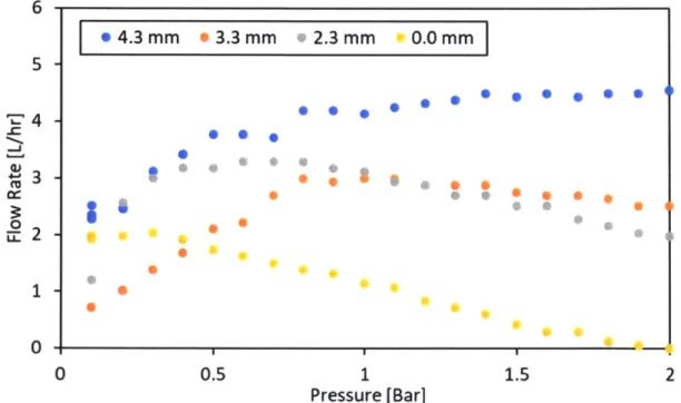
The data collected for each emitter is reported and grouped by common parameters. The data for emitters with a Y value of 0.5 mm is reported in Figure 8. Note that the data for the emitter with an X value of 3.3 is exhibiting behavior very different from the other three emitters, with an apparent activation pressure much later than the other emitters on this graph. It also exhibits very linear behavior before activation, rather than exponential behavior or behavior characterized by a square root. This caused there to be high errors in the fits detailed later in this thesis.
6 e 4.3 mm .3.3 mm .2.3 mm 0.0 mm 5 Me 3 -c 0 0 0.5 1 1.5 2 Pressure [Bar]
Figure 8: Experimental data from emitters with a Y value of 0.5 mm. Note the emitter with an X value of 3.3 mm is behaving differently from the other emitter performances in this
graph. It appears to activate much later (close to 0.8 bar) and behaves linearly before activation.
The data for emitters with a Y value of 1.0 mm is reported in Figure 9. The data in
emitters had a similar activation pressure, the slope of the data after activation was higher for emitters with higher values of X.
7 6 -> 33 i 2 1 0 0.0 mm I 4.3mm e3.3mm S
'1
0
ee 0 0 g0 0 0 * S. me * ~ ~ S e aI 0 0.5 1 0 0 0 1. 1.5 2 Pressure [Bar]Figure 9: Experimental data from emitters with a Y value of 1.0 mm. The data for emitters with a Y value of 1.5 is reported in Figure 10.
* 2.3 mm @00 5055 * @50 It & 0 ''' 0 a 8 7 6 5 4 3 2 1 0 0
IF *
4.3 mm 3.3 mm 2.3 mm 0.0 MM 1 Pressure [Bar] 0.5 1.5 2Figure 10: Experimental data from emitter with a Y value of 1.5 mm The data for emitters with an X value of 0.0 mm is reported in Figure 11.
.
4 I
4.5 4-3.5 --c 3-2.5 -. 2-o 1.5 - 1-0.5 - 0-I 0.5 mm * 1.0 mm * 1.5 mmI 00 * 0 * 0 S 0 4
;i ;;
e
i
:
:4is
43~I3*3* S a 0 *. *@@ S S 0.5 1 Pressure [Bar] 1.5 2Figure 11: Experimental data from emitters with an X value of 0.0 mm The data for emitters with an X value of 2.3 mm is reported in Figure 12.
g ** ge 00 *$w * * 0 0 0.0 * @0. 0 @004e *@0
e
0.5 mm 9 1.0 mm * 1.5 mm 0.5 1 Pressure [Bar] 1.5 2Figure 12: Experimental data for emitters with an X value of 2.3 mm The data for emitters with an X value of 3.3 mm is reported in Figure 13.
* e. 0 6 5 -c' -J 0 a: 4- 3- 21 -VI 0 -0
9 0 0 * 0. a 0.0 0.00. .100 55
0
OSOSa a a 0 0 0 00 * .0 0 5 0 0 1 0.5 mm * 1.0 mm * 1.5 mm 0.5 1 1 1.5 Pressure [Bar]Figure 13: Experimental data for emitters with an X value of 3.3 mm The data for emitters with an X value of 4.3 mm is reported in Figure 14.
0 0 0 S
I
0 0 .0 0 0. 0 0 0 0sI~
0 egS. 0 0 0 00 0 .0 0.0 000 .0 00 0 0 0.0 .00I5 I
8.a 6
0 e 0.25 mm * 0.50 mm . 0.75 mm - 1.00 mm e 1.50 mmI 0.5 1 1.5*
2 Pressure [Bar]Figure 14: Experimental data for emitters with an X value of 4.3 mm.
6 0
I
S S 0 0 0 2 7- 6-5. 4 1A-2
0-0 0 0 0 .9 0 .1 , 30 0 I5 Trends in the Overdamped Model
To create the overdamped model fit, the data collected was fitted to the equation:
Q(P) = AeBP - A + CP (1.4)
This equation is characterized by three parameters: A, B, and C. The fit was found using the Trust-Region algorithm of MATLAB's curve fitting toolbox. The trends of these parameters were then examined as dimensions in the emitter geometry X and Y were varied. Linear fits were then applied to the data to see if a positive or a negative trend could be identified. No more complex fits were applied due to the low amount of data for each fit. If a trend could be identified, it was examined to determine the trend's physical meaning. 5.1 Trends in Parameter A
Parameter A determines both the magnitude of the exponential part of the
overdamped model and the intercept of the activated linear part of the emitter behavior (Fig 15).
0
Pressure [Bar]
Figure 15: How varying variable A affects the performance of an emitter. All other variables being equal, two overdamped models are compared, one with a low A (a more negative A)
and the other with a high A (an A which is still negative but closer to zero) to show how variable A affects the model's performance. (Due to the nature of the overdamped model A
should never be positive).
The trendline for the data, shown in figure 16, showed a slight negative trend between parameters X and A, but the data in table 2 indicates it is not enough to conclude there is a negative trend with 95% certainty.
-2 -4 . E 120 a--6 -8 -10 -12' -1 0 1 2 X [mm] 3 4 5 high A low A / 3- --0.5mm Data Trendline 1.0mm Data Trendline 1mm Data Trendline * 0.5mm Data - 1.0mm Data * 1.5mm Data I I I
Figure 16: Trends in parameter A as parameter X varied. Note that each shows a slight negative trend for each trendline.
Y (mm) Slope (L/(hr- Lower Bound (L/(hr-mm)) Upper Bound
(L/(hr-mm)) mm))
0.50 -0.59 -4.08 2.90
1.00 -0.07 -0.75 0.61
1.50 -0.27 -0.78 0.25
Table 2: Slopes of the trendlines for parameter a as X varies. Upper and lower bounds are reported with 95% certainty. All slopes for the trendline were negative, but the upper bound uncertainties are all above zero, meaning we cannot be sure there is a negative
correlation between parameters A and X.
There was no discernible trend between variables Y and A, as is shown by figure 17 and table 3. . E 0 -2 -4 -6 -8
-o.Omm Data Trendline
-10 1
42
0 0.2 0.4 0.6 0.8 1 1.2 1.4 1.6 1.8 2
Y [mm]
Figure 17: Parameter A plotted as Y varies. Error bars are reported with 95% certainty. Note there is no clear positive or negative trend between parameters A and Y. X (mm) Slope (L/(hr- Lower Bound (L/(hr- Upper Bound
(L/(hr-mm)) mm)) mm)) 0.00 -0.876 -0.8907 -0.8613 2.30 0.314 -14.48 15.1 3.30 4.166 -25.38 33.72 4.30 -1.305 -3.286 0.6761 2.3mm Data Trendline -3.3mm Data Trendline -4.3mm Data Trendline * 0.0mm Data 2.3mm Data 3.3mm Data 4.3mm Data i ~ ~ I
Table 3: Slope of the trendlines showing how A varies depending on Y. The slopes of the trendlines are neither consistently positive or consistently negative, and so we cannot
conclude that there is any trend between parameters A and Y.
An examination of figures 16 and 17 shows a high error for the emitter with an X value of 3.3 mm and a Y value of 0.5 mm. The fit of the overdamped model on the data from this emitter (Fig 18a) provides insight as to why the fit for parameter A is particularly bad. Parameter A is responsible for the magnitude of the exponential part of the overdamped model and the intercept of the linear part of the overdamped model.
3.5 4 3 - * e * 3.5 -2.5 - 3 2 :i 2.5 2 1.5 -. 9 1.5 . - -Overdamped -overdampd 0.5 Data 0.5 data 0 0 0 0.5 1 1.5 2 0 0.5 1 1.5 2
a) Pressure [Bar] b) Pressure [Bar]
Figure 18: a) The overdamped model fit to the data of the emitter with a X value of 3.3 mm and a Y value of 0.5 mm. b) The overdamped model fit to the data of the emitter with a X value of 2.3 mm and a Y value of 0.5 mm. Part b) is included to contrast with part a as a
better fit. 5.2 Trends in Parameter B
Parameter B characterizes the rate at which the exponential part decays so the emitter begins exhibiting linear behavior (Fig 19).
(U
0
Pressure [Bar]
Figure 18: How the overdamped model differs, all other parameters kept the same, with a high B (negative with a lower magnitude) and a low B (negative with a higher magnitude).
(Due to the nature of the overdamped model, B should always be negative). As shown in figure 19 and table 4, there appears to be a slight positive correlation between parameters B and X, but the data did not confirm a positive correlation with 95% certainty. 0 -5 i-10 I-Ir-b -15 E 2-20 a. -0.5mm Dal 1.0mm Dat -1mm Data S0.5mm Dal S1.0mm Dat * 1.5mm Dal -251-aTrendline Trendline Trendline ..30 ' 1 I I -I --1 0 1 2 3 4 X [mm]
Figure 19: Graph depicting how parameter B varies with respect to parameter X. for each data point are reported with 95% certainty.
5
Error bars
high B
-low B
X Slope (hr/(L-mm)) Lower Bound (1/(Bar-mm)) Upper Bound (hr/(L-mm)) (mm)
0.50 3.617 -6.29 13.52
1.00 1.611 -3.85 7.07
1.50 1.447 -7.16 10.05
Table 4: Table of the slopes of the trendlines as parameter B varies with respect to parameter X. Upper and lower bounds are reported with 95% certainty. Note that though all slopes are positive, the lower bounds for the uncertainty bars for each negative meaning
we cannot conclude a positive correlation with 95% certainty. The slopes for parameter B as Y varies do not indicate a correlation between parameters B and Y, as shown in figure 20 and backed up by table 5.
10 -2.3mm O-.Omm Data Data TrendlineTrendline
-3.3mm Data Trendline 5 - -4.3mm Data Trendline O .Omm Data 0- 2.3mm Data S3.3mm Data -5 e 4.3mm Data -10 E-15 C20 - -25.-0 0.2 0.4 0.6 0.8 1 1.2 1.4 1.6 1.8 2 Y [MM]
Figure 20: A graph of how parameter B varied as Y changed. Error bars are reported with 95% certainty.
X (mm) Slope (1/(Bar-mm)) Lower Bound Upper Bound
(1/(Bar-mm)) (1/(Bar-mm))
0.00 mm 7.81 -4.00 19.62
2.30 mm -10.23 -16.18 -4.28
3.30 mm -16.49 -30.16 -2.81
4.30 mm 1.7 -11.25 14.65
Table 5: Slopes of the trendlines indicating how parameter B varies with parameter Y. The slopes are neither consistently positive or negative. Lower and upper bounds are reported
5.3 Trends in The Activation Pressure in the Overdamped Model
As stated before, the activation pressure of an emitter is calculated using parameter b in the overdamped model, described by equation 1.5.
PA =ln(0.0s) b (1.5)
When the activation pressure calculated by this equation is plotted against
parameter X, there appears to be a slight positive trend (Fig 21). However, an examination of the lower bounds of the fitted slopes indicates we cannot conclude there is a positive trend with 95% certainty (Table 6).
4 D Tr1nd -nI 0.5mm Data Trendline 3.5- 1.0mnm Data Trendline 1 --mm Data Trendline - 1.0mm Data 1.5mm Data i 2.5 -=0 1.5 --0.5 0 -1 0 1 2 3 4 5 X [MM]
Figure 21: Plot of how the activation pressure according to the overamped model varies with respect to X. Once again, the emitter with X=3.3 mm and Y=0.5 mm has a high
Y (mm) Slope Lower Bound (Bar/mm) Upper Bound (Bar/mm) (Bar/mm)
0.50 0.24 -1.64 2.11
1.00 0.025 -0.09 0.14
1.50 0.09 -0.26 0.431
Table 6: Slopes of the trend lines of how the activation pressure of an emitter varies with X according to the overdamped model. All upper and lower bounds are reported with 95%
certainty. The trendline slopes are all positive, but all lower bounds for the slopes are below zero, so we cannot conclude there is a positive correlation between the activation
pressure and X with 95% certainty.
When examining how the activation pressure varies with respect to variable Y, we do not observe any positive or negative trends, as shown in figure 22 and table 7.
4 1 T 0.0mm Data Trendline 2 -. 3mm Data Trendline -4.3mm Data Trendline D - 0.Omm Date 2-* 2.3mm Data 3.3mm Data * 4.3mm Data 1 -21 0 0.2 0.4 0.6 0.8 1 1.2 1.4 1.6 1.8 2 Y [mm]
Figure 22: The activation pressure according to the overdamped model as parameter Y varies. Error bars are reported with 95% certainty. Once again, the emitter with X=3.3 mm
Y Slope Lower Bound (Bar/mm) Upper Bound (Bar/mm) (mm) (Bar/mm) 0.00 0.078 -0.16 0.31 2.30 -0.44 -2.29 1.42 3.30 -2.56 -18.88 13.70 4.30 0.22 -0.37 0.81
Table 7: The slopes of the trendlines in the activation pressure according to the overdamped model as Y varies. Upper and lower bounds are reported with 95% certainty.
The slopes are neither consistently positive or negative, the lower bounds are all below zero, and the upper bounds are all above zero, so this data is not indicative of any trends. 5.4 Trends in Parameter C
Parameter C is the part of the overdamped model which corresponds to the slope of the emitter behavior after activation (Fig 23). This means that parameter C can be used to examine the uniformity of the emitter, where a C value closer to zero means better performance.
high C
- low C
0
Pressure [Bar]
Figure 23: How a changing parameter C affects emitter performance for a high parameter C (positive) and allow parameter C (negative).
Figure 24 indicates that there may be a positive correlation between parameters C and X, but the lower bounds of the slopes of the trendlines for the data only showed a 95%
certainty positive trend for one of the three Y values which were varied by X, as shown in table 8.
2
0
E-2 - -0.5mm Data Trendline
- 1.0mm Data Trendline
-Imm Data Trendline
*0.5mm Data
-3 -- 1.0mm Data
* 1.5mm Data
-1 0 1 2 3 4 5
X [mm]
Figure 24: Graph of how the variable C varies based on parameter X. The trendlines seem to indicate a positive correlation between C and X. Error bars are reported with 95%
certainty.
Y (mm) Slope Lower Bound Upper Bound
(L/(hr-Bar-mm)) (L/(hr-Bar-mm)) (L/(hr-Bar-mm))
0.05 0.2617 -1.618 2.141
1.00 0.4099 -0.333 1.153
1.50 0.3147 0.2517 0.3777
Table 8: Table of the values of the slopes indicating the trends of how parameter C vary with X. Note that two of the Y values'lower bounds are not below zero, meaning that while
a positive slope is more likely, we are not 95% certain of a positive slope for all three values.
When examining how parameter C varies based on parameter Y, it appears that there is a positive correlation between the two parameters, as shown in figure 25. However, the lower bounds for the slopes of the trendlines between parameters C and Y show that we cannot be 95% certain that there is a positive correlation between
3 2 U0 -1 0- -2 -3 -4 Figure 25: 0 0.2 0.4 0.6 0.8 1 1.2 1.4 1.6 Y [mm]
Trends in C with respect to Y. Note that the trends all seem to bars are reported with 95% confidence.
1.8 2
be positive. Error X (mm) Slope (L/(Bar-hr- Lower Bound (L/(Bar-hr- Upper Bound
mm)) mm)) (L/(Bar-hr-mm))
0.00 0.8245 -6.57 8.22
2.30 1.497 -5.59 8.59
3.30 2.96 -13.82 19.74
4.30 0.8736 -1.033 2.78
Table 9: Table of the values of the slope of the correlation between C and Y. Each shows a positive slope, though the lower bound is below zero, meaning we cannot conclude with
95% certainty that the correlation between C and Y is positive.
-0-m D t ... 2 .3mm Data Trendline 2.3mm Data Trendline -- 3.3mm Data Trendline - -4.3mm Data Trendfine O .Omm Data S2.3mm Data - e 3.3mm Data S4.3mm Data
6 Trends in the Piecewise Model
The fitted parameters i,
j,
and k of the piecewise model were examined for their correlations with the emitters' geometric parameters X and Y. The fit was found using the Trust-Region algorithm of MATLAB's curve fitting toolbox. The equation model with these parameters is given in equation 2.6.Q(P) = [iVfr x H (PA- P)] + [(j x P + k) x H(P - PA)] (2.15) 6.1 Trends in Parameter i
Parameter i in the piecewise model characterizes the pressure loss before the emitter enters its activated regime (Fig 26).
-high i
-low i
0
Pressure [Bar]
Figure 26: How changing Parameter i affects the piecewise model. A high i (positive and greater in magnitude) is compared to a low i value (positive but lesser in magnitude). (Due
to the nature of the model, i should never be negative.)
An examination of parameter i as it varies with parameter X does not reveal a clear trend between parameters i and X as shown by figure 27. As shown by table 10, the slopes are inconsistently positive or negative, the upper bounds are above zero for all but one value of Y and all lower bounds are below zero.
-0.5mm Data Trendline
10 1 1.mm Data Trendline
-imm Data Trendline
9- 0.5mm Data 1.Omm Data S1.5mm Data c 8- 76-3-1 2'I -1 0 1 2 3 4 5 X [mm]
Figure 27: Parameter i as it varies with parameter x. Error bars are reported with 95% certainty.
Y (mm) Slope (L/(hr-BarO.s-mm) Lower Bound Upper Bound (L/(hr-BarO-5-mm) (L/(hr-Bar-s-mm)
0.50 -0.21 -2.00 1.59
1.00 -0.45 -0.67 -0.22
1.50 0.25 -2.34 2.85
Table 10: Slope information for the trendlines of how parameter i varies with parameter X. Upper and lower bounds are reported with 95% certainty.
Parameter i seemed to show a slight positive trend when plotted by variable Y as shown in figure 28. However, table 11 shows that the lower bound for each trendline's slope is negative, so we cannot conclude there is a positive correlation with 95% certainty.
0 0.2 0.4 0.6 0.8
14
1 1.2 1.4 1.6 1.8 2
Y [mm]
Figure 28: Trends in parameter I as parameter Y varies. Error bars are reported with 95% certainty.
X (mm) Slope (L/(hr-Bar. 5- Lower Bound Upper Bound mm) (L/(hr-Bar-5-mm) (L/(hr-BarO.5-mm)
0.00 0.97 -14.18 16.11
2.30 1.53 -2.69 5.75
3.30 6.65 -2.95 16.25
4.30 1.65 -0.25 3.56
Table 11: Trends in the trendlines of how parameter i varies with Y. All upper and lower bounds are reported within 95% certainty.
6.2 Trends in
j
Variable
j
characterizes the slope of the activated regime of an emitter in thepiecewise model (Fig 29). This means that variable
j
can be used to judge uniformit, where aj
closer to zero is more desirable.S2.3mm-3.3mm Data Tren -4.3mm Data Tren -. mm Data 2.3mm Data 3.3mm Data 12 V10 8 4 E . 0 -2 dline idline dline idline T~ . . . .
-high j -low j
0
Pressure [Bar]
Figure 29: How parameter
j
affects the piecewise model. A highj
(positive) is compared to a lowj
(negative).In examining how
j
varies with respect to X, the trendlines consistently showed a postitive trend as shown in figure 30. However, the the lower bounds for the slopes of these trendlines were all below zero as shown in table 12. This means that we cannot conclude with 95% certainty that there is a positive trend between parametersj
and X.1.5 -0.5mm Data Trerdline 1.0mm Data Trendline -1mm Data Trendine 1 0.5mm Data e 1.0mm Data * 1.5mm Data 10.5 E-0.5 1.5 -1 0 1 2 3 4 5 X [mm]
Y (mm) Slope (L/(Bar-mm-hr)) Lower Bound Upper Bound (L/(Bar-mm-hr)) (L/(Bar-mm-hr))
0.50 0.35 -0.23 0.93
1.00 0.17 -0.04 0.38
1.50 0.27 -0.48 1.03
Table 12: Slopes of the trendlines of how
j
varies as X increases. Lower and upper bounds are reported with 95% certainty.When examining how
j
varies with Y, there appears to be a positive correlation between variablesj
and Y, as shown in figure 31. However, as shown by table 13, only one of the four trendlines' slopes do not have a negative lower bound, so we cannot becompletely sure that there is a positive correlation.
2 .5 0.5 - 0--5- .0mm Data Trendline - 23.3mm Data Trendline -3.3mm Data Trendfine --. 3mm Data Trendline > -1 O .Omm Data -2.3mm Data -1.5 9 3.3mm Data -1.5* 4.3mm Data -21- II 0 0.2 0.4 0.6 0.8 1 1.2 1.4 1.6 1.8 2 Y [mm]
Figure 31: Trends in
j
as Y varies. Error bars are reported with 95% certainty.X (mm) Slope (L/(Bar- Lower Bound Upper Bound
mm-hr)) (L/(Bar-mm-hr)) (L/(Bar-mm-hr))
0.00 1.26 -3.25 5.78
2.30 0.81 -9.14 10.77
3.30 1.16 -0.22 2.55
4.30 0.95 0.51 1.40
Table 13: Table of the slopes of the trendlines of how j varies as Y increases. Upper and lower bounds are reported with 95% certainty.
The parameter k in the piecewise model represents the intercept of the activated regime of the emitter (Fi
a/
g 32).
high k
-low k
Pressure [Bar]
Figure 32: How a changing parameter k affects the performance of the piecewise model. A higher k value (positive and with greater magnitude) is compared to a lower k value (positive with lesser magnitude). (Due to the nature of the piecewise model, k should
never be negative).
Examining how k varies with X reveals a slight positive trend, as shown in figure 33. However, table 14 shows that two of the trendlines for the relationship between k and X had lower bounds below zero, so we cannot say with 95% certainty that the correlation between k and X is positive.
6 0.5mm Data Trendline 1.0mm Data Trendline 5.5 -1mm Data Trendline -0.5mm Data 5 - .Omm Data V 1.5mm Data J-:4.5 2 -ET J! 3.5 --1 0 1 2 3 4 5 X [mm]
Figure 33: Trends in parameter k as parameter X varies. Error bars are reported with a 95% certainty.
X Slope (L/(hr-mm)) Lower Bound (L/(hr-mm)) Upper Bound (L/(hr-mm)) (mm)
0.50 0.33 -0.56 1.22
1.00 0.47 0.02 0.93
1.50 0.31 -1.04 1.66
Table 14: Slopes of the trendlines of how parameter k varies with x. Lower and upper bounds are reported with 95% certainty.
Examining the trends in k when Y varies there appears to be a positive slope, as shown by figure 34. Table 15 however shows the the lower bounds for the slopes of each of the trendlines are below zero. Therefor, we cannot conclude with 95% certainty that the correlation between parameters k and Y is positive.
6 5.51 5 4.5 4 3.5 3 2.5 2 0 0.2 0.4 0.6 0.8 1 1.2 1.4 1.6 1.8 2 Y [mm]
Figure 34: Trends in parameter k as parameter Y varies. Error bars are reported with a 95% certainty.
Y (mm) Slope (L/(hr-mm)) Lower Bound Upper Bound (L/(hr-mm))
(L/(hr-mm))
0.00 0.23 -4.00 4.47
2.30 0.77 -18.63 20.17
3.30 0.19 -9.66 10.03
4.30 1.16 -1.36 3.67
Table 15: Table of the slopes of the trendlines of how j varies as Y increases. Upper and lower bounds are reported with 95% certainty.
6.4 Activation Pressure According to the Piecewise Model
In examining how the activation pressure according to the piecewise model varies with X, figure 35 indicates a positive slope, but table 16 shows that we cannot be certain of a positive trend with 95% certainty.
-0.0mm Data Trendline - 2.3mm Data Trendline -3.3mm Data Trendline -4.3mm Data Trendline * 0.0mm Data 2.3mm Data * 3.3mm Data - 4.3mm Data I
I-p p p p p p p I I I I I5 4 cc m 3 2 0 0 -29 -1 0 1 2 3 4 5 X [mm]
Figure 35: Activation pressure according to the piecewise model of performance of each emitter as X varies. Error bars are reported within a 95% certainty. There is no clear trend,
with the slopes of the trendlines tending close to zero.
Y Slope as X varies Lower Bound (Bar/mm) Upper Bound (Bar/mm)
(mm) (Bar/mm)
0.50 0.15 -0.28 0.58
1.00 0.24 -0.17 0.65
1.50 0.07 -0.31 0.44
Table 16: Lower and upper bounds of the slopes of the trendlines for activation pressure according to the piecewise model of performance of each emitter as X varies. There is no clear trend, with the slopes of the trendlines tending close to zero, the upper bound of the
slope being above zero and the lower bound of the slope below zero.
The data on how the activation pressure according to the piecewise model does not indicate a clear trend, as shown in figure 36 and table 17.
[-0.5mm Data Trendline -- 1.0mm Data Trendline - 1. mm Data Trendline 0.5mm Data 1.umm Data-e. 1.5mm Data .1 i I I I a a I a I
-5 4 3 2 b. -I 0 Z1 -9 -. mm Data Trendline -2.3mm Data Trendline -3.3mm Data Trendline -4.3mm Data Trendline - e 0.Omm Date 2.3mm Data 3.3mm Data -4.3mm Data .-... 0 0.2 0.4 0.6 0.8 1 1.2 1.4 1.6 1.8 2 Y [mm]
Figure 36: The activation pressure plotted as it varies with Y according to the piecewise model. Error bars are reported with 95% certainty.
X (mm) Slope (Bar/mm) Lower Bound (Bar/mm) Upper Bound (Bar/mm)
0.00 0.01 -0.13 0.15
2.30 0.02 -3.99 4.02
3.30 -0.94 -1.45 -0.43
4.30 0.21 -1.00 1.41
Table 17: The slopes of the trendlines of how the activation pressure varies with Y according to the piecewise model. Upper and lower bounds are reported with 95%
7 Comparison of the Piecewise and Overdamped Models
In order to compare the piecewise and overdamped models, the average
uncertainties of key emitter characteristics were compared. In comparing the uncertainty of the activation pressure of each model, the overdamped model was found to have a significantly lower average uncertainty, as shown by figure 37. This makes sense, as in the overdamped model the activation pressure is dependent on only one variable, whereas in the piecewise model three variables must be used to calculate the activation pressure, and the propagation of uncertainties causes the uncertainty for the activation pressure to be even greater. 1.8 1.6 -t 1.4 U r- 1.2 1 UCO 0.8 4-. M 0.4 LI 0.2 0 m Piecewise * Overdamped
Figure 37: Comparison of the average uncertainty of the activation pressure according to the piecewise model and the overdamped model. Error bars are reported with 95%
certainty.
The uniformity for the piecewise model is characterized by parameter
J,
while the uniformity for the overdamped model is characterized by parameter C. When thethat the piecewise model reported the slope after an emitter's activation with less
uncertainty. However, as indicated by figure 38, we cannot conclude 95% certainty that the piecewise model provides a more certain representation of the emitter's uniformity.
0.5 0.4 U 0U M 0.2 0.1 0 m Piecewise * Overdamped
Figure 38: Comparison of the average uncertainty of the parameter informing the emitter's performance after activation for the piecewise and overdamped model. Error bars are
reported with 95% certainty.
This indicates that overall, the overdamped model provides more certain results, particularly with regards to the activation pressure. Though the piecewise model may provide a more certain characterization of the uniformity of an emitter, the data does not show that this model is significantly more certain.
8 Secondary Test: Varying Sinusoidal Shape Depth
In section 6, a variety of trends were identified by examining emitters with
rectangular prism chambers under the membrane. However, we expect the membrane to deform in a curved shape as it is simply supported by a ledge on each side. A second set of experiments was run to examine whether the trends identified in section 6 of this thesis could be identified when a different shape is under the membrane. In this experiment, rather than a rectangular prism beneath the membrane, the cavity beneath the membrane has a sinusoidal shape. Similar geometric parameters were varied in this test, as shown in figure 39. The first parameter was W, the distance between the outlet hole and the center of the chamber under the membrane. W is analogous to X from the tests described in section 6 of this thesis. The second parameter was Z, the distance between the lowest point of the chamber under the membrane and the bottom of the undeformed membrane. Z is
analogous to parameter Y from the tests described in section 6 of this paper.
W
1Z
Z
a)
I
I
b)L__
Figure 39: Diagrams indicating the physical meaning of parameters W and X regarding the emitter geometry. a) Parameter W is the distance between the outlet hole and the center of
the chamber under the membrane. b) Parameter Z is the distance between the bottom of the undeformed membrane and the lowest point in the chamber under the membrane.
Four emitters with sinusoidal chambers were made and tested. The four emitters' dimensions are listed in table 18.
Z=0.5 mm Z=0.5 mm
W=0.0 mm W=4.3 mm
Z=1.5 mm Z=1.5 mm
Table 18: W and Z values for each sinusoidal emitter. Note that there is no data for the emitter with a W value of 0.0 mm and a Z value of 0.5 mm because the emitter would not
emit water at any pressure between 0 and 2 Bar. 7.1 Flow Rate Data for Sinusoidal Emitters
Data collected from the sinusoidal emitters is reported in figure 40. 4.5 . W=0.0 mm Z=1.5 mm 4 -W=4.3 mm Z=0.5 mm 3.5 - W=4.3 mm Z=1.5 mm 2.5 0 15 0.5-0 0 0.5 1 1.5 2 Pressure [Bar]
Figure 40: Flow rate data for the sinusoidal emitters. 7.2 Activation Pressure
In the square testing, no trend was observed between the activation pressure according to piecewise model and Y. Examining how the activation pressure according to piecewise model varies with Z in a sinusoidal shape, however, the sinusoidal shape with a greater depth had a higher activation pressure, as shown by figure 41.
0.3 . 0.25
I
2 0.2 0.15 0.1 J CU 0.05I
m W=4.3mm Z=1.5mm m W=4.3mm Z=0.5mmFigure 41: Comparison of the activation pressure according to the piecewise model of an emitter with an W value of 4.3 mm and a Z value of 1.5 mm and an emitter with a W value of 4.3 mm and a Z value of 0.5 mm. Error bars are reported with 95% confidence. The data
indicates that the emitter with a greater Z value had a statistically significantly higher activation pressure.
In square testing, a positive trend was observed between the activation pressure according to the piecewise model and X. Examining how the activation pressure varies with W, the activation pressure of the emitter with a greater W was observed to have a greater activation pressure. This is shown in figure 42.
0.3 ' 0.25 0.2 -0.15 0.1-
<0.05-F
W=O.Omm Z=1.5mm n W=4.3mm Z=1.5mmFigure 42: Comparison of the activation of the activation pressure according to the piecewise model of an emitter with an W value of 0.0 mm and a Z value of 1.5 mm and an
emitter with an W value of 4.3mm and a Z value of 1.5 mm. The lower bound of the activation pressure for the emitter with W=4.3mm is 0.22 Bar, which is identical to the upper bound of the activation pressure of the emitter with W=O.Omm to one hundredth of a millimeter. This means that while we just barely can't conclude there is a difference with 95% certainty, there is evidence for a difference with a slightly lower degree of certainty.
Examining the activation pressure of the sinusoidal shaped emitters according to the overdamped model did not reveal any trends due to the high uncertainties, shown by
figure 43. 10 -1 -2 -3 4 3 2 -1 -2 -3 a) 4' ' b) -4
Figure 43: a) Comparison of the activation pressure according to the overdamped model of an emitter with an W value of 4.3 mm and a Z value of 1.5 mm and an emitter with an W
value of 0 and a Z value of 1.5 mm. Error bars are reported with 95% certainty.
b) Comparison of the activation pressure according to the overdamped model of an emitter
with an W value of 4.3 mm and a Z value of 0.5 mm and an emitter with an W value of 4.3 mm and a Z value of 1.5 mm. Error bars are reported with 95% certainty.
7.3 Uniformity
The high uncertainties in the calculated value for parameter
j
meant that we could not observe any difference between the parameterj
as W varied, as shown in figure 30.0.1 .Z" 0 -0.1 W -0.2 E LM -0.3 -0.4 * W=0.Omm Z=1.5mm a W=4.3mm Z=1.5mm
Figure 44: Comparison of parameter
j
between an emitter with W=4.3 mm and Z= 1.5 mm and an emitter with W=0.0 mm and Z = 1.5 mm. Uncertainty bars are reported with 95%certainty.
In the square emitter testing, a positive trend was observed between parameters Y and j. It was found that the emitter with a greater Z had a higher j value by a statistically significant amount, as shown by figure 45.
0 -0.1 -0.2-C -0.4 E -0.5 -J -0.6
I
W=4.3 mm Z=1.5 mm EW=4.3 mm Z=0.5 mmFigure 45: Parameter j compared between an emitter where X=4.3 mm and Y=0.5 mm and am emitter with X=4.3 mm and Y =1.5 mm. Error bars are reported with 95% certainty.
In the square testing, a positive trend was observed between parameters C and Y. It was also found that the sinusoidal emitter with a greater Z value had a statistically
significantly greater C value. This can be seen in figure 46.
CO E -J 0 -0.1 -0.2 -0.3 -0.4 -0.5 -0.6
.I
I
W=4.3 mm Z=0.5 mm U W=4.3 mm Z=1.5 mmFigure 46: Parameter C for an emitter with W=4.3 mm and Z=0.5 mm and an emitter with W=4.3 mm and Z=1.5mm. Error bars are reported with 95% certainty.
In the square emitter testing a positive trend was observed between parameter X and parameter C. Similarly, the sinusoidal emitter with a greater W also had a greater C value, though not by a statistically significant amount. This is shown in figure 47.
0 -0.2 -0.4 E -0.6 -0.8 IE W=4.3 mm Z=1.5 mm N W=0.0 mm Z=1.5 mI
Figure 47: Parameter C for an emitter with W=4.3 mm and Z=1.5 mm compared to an emitter with W=0.0 mm and Z=1.5 mm. Error bars are reported with 95% certainty.
9 Conclusions
Between the overdamped model and the piecewise model, the overdamped model generally had lower uncertainty values, indicating that it may be a useful tool to model emitters in the future. While none of the trends in emitter parameters were sufficient to create a predicative model for emitter behavior, certain trends in emitter behavior were observed which may inform emitter design. The activation pressure revealed similar results through both the overdamped and the piecewise model. While there was no discernible trend between the activation pressure and y, there was some evidence of a positive trend between the activation pressure and parameter X. While this could not be confirmed with 95% certainty, it does indicate that an outlet hole directly under the center of the membrane results in an emitter with the lowest activation pressure. The slope of the activated portion of the emitter, characterized by parameter C in the overdamped model and parameter
j
in the piecewise model, was shown to have a positive trend with both X and Y, though we could not confirm this trend with 95% certainty. Similar trends were observed in the sinusoidal emitters, however, providing more evidence for this trend. This provides a guideline for how the uniformity of an emitter can be improved if the slope after activation is too high or too low.10 Appendices
Appendix 1: Emitter dimensions 2 49 -- -.--- 4xRO.75 4X 04.98 3X01.50 -4XRI 24 20.15 18.8 12 14XR1.50 11-51 151 21 2- - 4 - -f ! I6.35 5.23 6.35-1.75] 1.7 5 + Y L ~ 16.26-16.88 26.92 - X -26.98--- 28.484 29.10--- -31.23 -- 42.65-43.75 5.26 3.21 0.21 )C Rs HmBME ED:.21 20.15 -TOE-CB: 30.35 12.07 0 15.18 27 -3.50
SL
Alumium1
B
A
1 BA
6.05 f 1,502
10 Acknowledgements
I would like to thank Professor Amos Winter for the opportunity to pursue this Thesis. I would also like to thank Julia Sokol and Jeffery Costello, whose advice and guidance have been invaluable.
11 References
[1] Sivanappan, R.K., 1994, "Prospects of micro-irrigation in India," Irrigation and Drainage Systems, vol. 8.
[2] Nkya, Kam; Mbowe, Amana; Makoi, Hoachim H.J.R., 2015, "Low-Cost Irrigation Technology, in the Context of Sustainable Land Management and Adaptation to Climate Change in the Kilimanjaro Region," Journal of Environment and Earth science, vol. 5, No. 7.
[3] Shamshery, Pulkit; Winter V, Amos G., 2018, "Shape and Form Optimization of On-Line Pressure-Compensating Drip Emitters to Achieve Lower Activation Pressure," Journal of Mechanical Design, vol. 140.
[4] Burt, Charles M.; Feist, Kyle, "Pressure Compensating Emitter Characteristics," Irrigation Association, from
https://www.irrigation.org/IA/FileUploads/1A/Resources/TechnicalPapers /2013/ PressureCompensatingEmitterCharacteristics.pdf
[5] Bequette, Wayne B., 2002, "Process Control: Modeling, Design, and Simulation," Prentice hall PRT.
[6] White, Frank M., 2008, Fluid Mechanics, McGraw-Hill, New York.
[7] Zazueta, Fedro S. "Understanding the Concepts of Uniformity and Efficiency in Irrigation," University of Florida, from
http:I/irrigationtoolbox.com/ReferenceDocuments/Extension/Florida/AE36400.p
df
[8] Narain, Jaya and Amos, Winter G., 2018, "A Hybrid Computational and Analytical Model of Irrigation Drip Emitters," ASME 2018 International Design Engineering Technical Conferences and Computers and Information in Engineering Conference, Volume 2B: 44th Design Automation Conference.