CABIOS
Vol.7, no.2. 1991Pages 155 - 160GEOBASE: a simple geographical information
system on a personal computer
Philippe Blaise and Cesare Gessler
Abstract
Spatially distributed data are often encountered in the biological sciences. Representation and analysis of such data requires specific tools. A simple geographical information system is presented, which allows representation and elementary analysis of geographically coded information. The system handles two kinds of data: maps and facts, where map data describe the basis on which the fact data are located. Maps consist of objects described through a set of coordinates, while for facts a coordinate pair is associated with an unlimited number of data records containing five fields: a date, an element from a list, a two-character code, an integer number and a real number.
The input data can be displayed interactively on screen by logically combining selection criteria for each field. The facts corresponding to the selected criteria are either displayed as such, or are clustered and displayed as polygons or pies. A short example showing a possible application of the program is presented and advantages as well as limitations are discussed.
Introduction
Many applications in biological sciences are concerned with spatial data, e.g. geobotanical studies or population dynamics in pest management, and there is often a need for analysis of spatial distribution patterns. In plant disease epidemiology, analysis of spatial data is required for restricted scale studies such as analysis of patterns of spread of soil-borne pathogens or for large-scale studies dealing with the spread of airborne pathogens that can travel over hundreds of kilometers.
Working with data that include a spatial component is difficult since quantification is not reduced to a single value. Special tools are therefore required, which are commonly called geographical information systems (GISs). A GIS is distinguished from other data management systems by its inherent ability to maintain spatial relationships of variables as well as their attributes.
Since the appearance of the first GISs in the 1960s, there has been a rapid increase in their number. To date, a wide variety of systems have been developed, primarily for land-use planning and natural resource management at the urban, regional, state and national levels of government, but also for applications by public utilities and private corporations (Smith
Institute of Plant Sciences/Phytomedicine, Swiss Federal Institute of Technology, Universitatstrasse 2, 8092 ETH-Zurich, Switzerland
etal., 1987). Although the existing systems can and have been
used for biological studies, their primary use focuses rather on the geographical than on the biological side of the problems. These are most sophisticated, very powerful packages, which in turn require trained and skilled users. They run mainly on minicomputers or mainframes, often only on special adapted hardware and a personal computer version exists for only a few of them.
We present here a simple GIS with limited geographical features, powerful enough to handle large data sets and with characteristics that should appeal to biologists who do not have the need for a professional GIS.
System and methods
The program was developed on an IBM PC-AT with 640 kbytes of RAM, a hard disk, a mouse and an EGA color display. It was written in Pascal, and compiled with the Turbo-Pascal compiler version 5.0 (Borland International, 1988).
The recommended configuration to run the program is an IBM PC-compatible computer with at least 512 kbytes RAM, an EGA or VGA graphics adapter with a colour display, a hard disk and a mouse. The use of an 80x87 mathematical coprocessor enhances the speed by a factor of 2 on average. The program also runs with CGA, MCGA and Hercules graphics adapters. However, since these do not support colours, the use of the program in visualizing facts on screen is greatly reduced. In the same way, one can dispense with the hard disk and the mouse, but this again limits the usefulness of the program.
Limitations: Since the map files are kept on disk, their size is restricted only by the available space and/or the limitations of DOS. The fact files (see below) are kept in memory are are thus subject to the data structure limitations of the compiler. This means that the maximum amount of facts (coordinate pairs) is limited to 16 384. The number of information records for each of these facts is limited only by the available disk space. Maps can be currently printed on Postscript laser printers or plotters using the HPGL command set. The outputs presented were produced on a TI 2108 laser printer.
Implementation
Geobase is an unconventional GIS in the sense that it distinguishes two kinds of data: maps and facts.
Maps represent the canvas on which the facts are located. They are composed of objects described through a name, a set of coordinate pairs and attributes describing the way these co-ordinates are connected together (e.g. line, closed line, filled surface). Although maps are used usually as the equivalent of geographic maps and composed of geographical objects such as borders, rivers or lakes, they can also describe any spatial structure, e.g. a field, where the objects could be: the border of the field, regions of the field with special soil characteristics, trees, etc.
Facts correspond to collected data and differ from map objects in three ways:
(i) Each fact contains an unlimited number of information records.
(ii) The description of the localization of facts in space is (currently) limited to one coordinate pair so that the information content of a fact is associated either with a single point or with a rectangle or a circle centered on this point,
(iii) Facts can be selected from their information content for display or clustering.
To simplify entry and data structure, the number of fields per record is fixed. Each record consists of up five fields: the first is a date field, which will be used usually to keep track of either the date at which the recording was made or at which the record was entered; the second field contains an element out of a user-defined list (e.g. cultivar) and the other fields contain a code (two characters), an integer number (—32 768 to + 32 768) and a floating point number (±1.5 10"45 to
3.4 1038).
A computer-based GIS may be viewed as having five component subsystems (Knapp, 1978), including: data encoding and input processing; data management; data retrieval; data manipulation and analysis; and data display.
These different subsystems will be presented briefly, and Figure 1 shows a schematic representation of the menu tree through which the user selects the different functions.
Data input
Maps are input by entering the coordinate sets defining each object. This can be tedious if many coordinates have to be entered; however, two features reduce this handicap: (i) The program can import coordinates from ASCII files,
so that already existing data need not be input again, (ii) Map files may be edited and appended at any time, i.e.
a very simple map composed of just a few points can be input first and extended later.
The location of facts can be entered either by typing in the coordinates or by 'clicking' on the map with a mouse. The latter is not so precise, but may be sufficient for some applications. Once the location and the first information record of a fact has been input, additional records may be added, again either by
Geobit
Ed* facts Convert tacit fUe Append facts to • Tacts fDe Create Dew fans We
Enter coonUoMes I Clict oo map |
Move roan
D«a editor E^u/Append f*cu Load new set of f »cu
Select mis file Append to map fUe Create oew imp PDecoBvenkn
Eo*crcoortaiates| hepon firm (lie |
Display selected facts Set t e h x t l o i cmcTia Select field to display Ouster Tacts Select new fact Hie m f o o n Tacts Tom ofT display oT tacts
Prin m i e n ! display Set die of primed map Select decimal km
How to display.. -Mtp display level Set colon
Mspiiie
Fig. 1. Schematic representation of the menu tree of Geobase. Each rectangle
represents a menu or submenu. For clarity, lowest-level menus are omitted.
selecting the coordinates, or by 'clicking' at the location of that fact on the display.
Data management
Special functions allow management of maps and facts data. They can be exported or imported via the ASCII format, edited or appended.
Data retrieval
Apart from the export of data mentioned above, data are retrieved through the graphic display: when displayed, each fact can be addressed by 'clicking' on its location. The description of this fact is then displayed and the user can browse through the available records if more than one has been entered.
Data analysis
Simple analyses of facts can be made either on facts handled and displayed separately or on clusters of facts whereby the distance between two facts is used as a clustering criterion. The values associated with facts can be divided into classes, and then the single classes are selected for display or not. This allows queries to be answered by combining logically the different characteristics of the facts. For a survey of diseased bean fields (see example below), such a query could be: select all bean fields which in 1987 were sown with the variety X or Y, had a total disease severity of at least 10%, where plants grew to a normal height, and display them with colours corresponding to the disease severity classes. In the case of clusters, the program calculates the proportion of facts belonging to each class, within a cluster.
Data display
The display of facts on maps is the most important part of Geobase. The user looks at the current map and selected facts
A simple CIS on a personal computer
Fig. 2. Printout of the map used in a field study on bean diseases at a scale of 1:2 500 000. The map shows border, main lakes and rivers of Switzerland.
Because of size contraints, cities and highways are not represented. Bean fields are displayed as spots, mainly in the northern part of the map.
through a window defined by its centre and an associated scale. The centre of the current viewing window is selected by pointing on it or by entering its coordinates directly, and the scale is set either by selecting a previously fixed scale, entering a free scale or zooming in or out, which corresponds to halving or multiplying the current scale by a factor of 2. These operations allow a precise positioning of the viewing window. In the case of maps containing many objects and thus requiring a longer time to display, classes of objects can be selectively inactivated until the desired scale and location are found. Facts are overlaid on the map as dots, characters, circles or rectangles depending on the user's selection. Clusters are displayed as polygons enclosing the facts belonging to each cluster, or as pies divided according to the number of facts in each class of the informa-tion field selected for display.
Hard copies are output in two steps: first, the size of the printed map is entered in centimeters, which determines the size of the viewing window on the screen (since the screen has a limited size, the window occupies the greatest possible surface by respecting the size ratio between the sides; the selected scale is thereby maintained) and then the desired map content can be built interactively, by moving the centre of the window, changing its associated scale and selecting the map objects or facts to display.
Great care has been taken to develop a user-friendly inter-face, so that the program can be mastered in a short time by
a user without computer experience. All operations are performed through menus where the selection can be made either with a mouse or through the keyboard. All functions are performed interactively. The coordinates corresponding to the location of the mouse pointer are displayed constantly, which allows very precise work.
Ejcample
The following example shows a simple application of Geobase. A study on a new disease in bean crops (hull spots) in Switzerland was initiated in 1986. Since this disease seemed to be corrrelated with numerous factors such as cultivar, occurrence of Alternaria disease or microclimate of the field location concerned, a comparative study involving > 150 fields was started to obtain more indications of the possible correla-tions between these factors and the incidence of the disease. Geobase was chosen as a tool to keep track of the field locations and to produce status reports. Moreover, it allowed rapid testing of possible causal hypotheses.
The map used was of Switzerland and contained the information necessary for the user to locate the fields, such as borders, rivers, lakes, cities and highways.
The facts were in this case single fields, and the information recorded for each field was: date of record, cultivar, general state of the crop at harvest, accumulated disease severity level
- A
• W o h l >
• W o h l .
Fig. 3. Printout of the northern part of the map used in a field study on bean diseases at a scak of 1:500 CXX). (A) Bean fields arc displayed as spots in a grey level corresponding to the disease severity at harvest (darker spots correspond to higher severity levels). (B) Result of clustering the bean fields with a maximal distance of 4000 m. The pies are centered on the center of gravity of the corresponding cluster. Their size is proportional to the number of fields belonging to the cluster and the different sectors correspond to the disease severity classes: 0 - 5 , 5 - 2 0 , 2 0 - 5 0 , 5 0 - 8 0 , 80-95% (increasing grey levels represent higher severity levels).
for all diseases and severity level due to the pathogen Alternaria. Figure 2 shows an overview (scale 1:2 500 000) of the map with the bean fields mostly in the northern part of the country.
A closer look at this part is given by Figure 3(A) (scale 1:500 000), while Figure 3(B) shows the same region after clustering with a maximal distance of 4000 m between fields.
A simple CIS on a personal computer
Function OulaNi(PoJnt)-.fatoger
dDOT 10 ^^^nlCU i^Oim ]
( belongs w w o if it doe* not belong yet to my clnjtsr ) {
For til Pomti P do
If CbMath<Jr)-0 then cnate new cluki
For til pofat* R for which R, - Pi < Mixdi* do If Oiutedfa(R)>0 or CkumNi(R) # CbutaNi<P) tfa«n
If Ounce between R « d P < Madim then S CbutaNi(RH) then R bdoap to OaitaNKP)
ebe Join Clutertb(R) to ChuCeiNr(P) Bud
Fig. 4. Pseudo-code of the algorithm used to cluster facts in the program Geobase. Each point P is defined through a coordinate pair (PX,P) and points
are sorted after the Px coordinate. A cluster is composed of all points not further
apart from the next one than the maximum distance Maxdist.
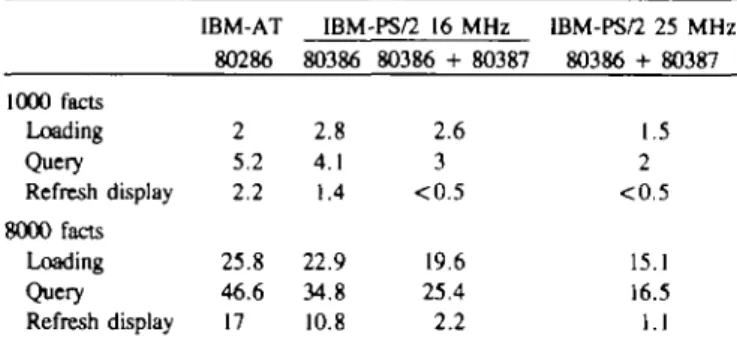
Table I. Computation time in seconds for different actions taken in the program
Geobase. 1000 facts Loading Query Refresh display 8000 facts Loading Query Refresh display IBM-AT 80286 2 5.2 2.2 25.8 46.6 17 IBM 80386 2.8 4.1 1.4 22.9 34.8 10.8 -PS/2 16 MHz 80386 + 80387 2.6 3 <0.5 19.6 25.4 2.2 IBM-PS/2 25 MHz 80386 + 80387 1.5 2 <0.5 15.1 16.5 1.1 The tests were run on four different computers with different microprocessors with two data sets containing 1000 and 8000 facts
The pies show the frequency of the different classes of total field disease severity.
Algorithms
The structure of the map data is a cartographic structure, i.e. no spatial relationships are stored among objects. The single map objects are described through a vector model. Such a structure is commonly defined as a 'spaghetti' structure. To introduce some ordering in the map files, similar structures are grouped together within a file, and information on the location of the objects is stored, thus speeding up the retrieval and display process.
The facts data are stored in two separate files. The first contains the coordinates defining the location of the facts and pointers to the stored information on each fact in the second file. During working, the coordinates of the current data set are kept in memory. To speed up access to the facts falling in the selected range of coordinates, their coordinates are sorted in ascending order of x coordinate values. To avoid re-sorting each
time a data set is loaded, the sorted coordinates are stored in a third file. Coordinates are sorted by the quicksort algorithm (Sedgewick, 1988).
A simple algorithm has been developed to cluster the facts. The primary goal was to limit computations of distances between facts, since each computation involves square roots and multiplications. A pseudo-code version of the clustering algorithm is given in Figure 4.
The convex hull around a cluster of facts is computed with the algorithm described by Sedgewick (1988).
Zooming is achieved through definition of viewports and associated world coordinate systems as usual in interactive graphic interfaces (Foley and Van Dam, 1983; Rogers, 1985).
Discussion
Scientists and engineers have long understood the importance of pictures in perceiving and communicating functional relationships in quantitative data. Geographic information systems have been used successfully in several disciplines such as soil science, forestry, geology, landscape architecture and entomology. Their applications are increasing and it is estimated that -4000 GISs will be operational by 1990 in North America (Tomlinson, 1984). Although the program presented here does not pretend to compete with professional GISs, it has some features that make it useful for the biologist's daily work: its easy stnicture and user interface shorten the necessary training time, the map structure allows work with even small amounts of map information and its implementation on a microcomputer makes it a decentralized, affordable tool. There is a price to pay, however, for these advantages:
(i) The number of functions available is limited, partly because spatial relationships between map objects are not considered—a primary drawback of the vector type data model. On the other hand, this data model is more compact than tesselation-type data models, and there are more algorithms available for vector models than for others (Peuquet, 1984).
(ii) Since computation time increases with map precision and numbers of facts, working with large data sets on PCs with limited power could become very slow. However, we used Geobase for a survey of plane trees in Southern Switzerland where > 8000 trees were recorded with their healthy state (Blaise and Gessler, 1988), and did not encounter real speed problems on AT-type machines (Table I). From this point of view, the maximum number of facts that the program can handle may be seen as a reasonable limit.
(iii) The input of map data is not automated. This has not been a problem so far, but could become so if descriptions of large maps have to be input. The possibility of importing coordinates of map objects from ASCII files should, however, provide a way around this obstacle.
Acknowledgements
We thank Dr M.S.Wolfe for critical reading of the manuscript and G. Eich for kindly providing the data used in the figures. The technical assistance of B.Koller in implementing the support for Postscript laser printers is gratefully acknowledged.
References
Blaise,P.H. and Gessler.C. (1988) Disease mapping on PC: application to the canker stain of plane trees in southern Switzerland. Abstracts, 5th International Congress of Plant Pathology, Kyoto.
Knapp.R. (1978) LANDSAT ancillary data input to automated geographic information systems. Report no. CSC-CR78-6019. Computer Science Corporation, Silverspring, ML.
FoleyJ.D. and Van Dam,A. (1983) Fundamentals of Interactive Computer
Graphics. Addison-Wesley, Reading, MA.
Peuquet.D.J. (1984) A conceptual framework and comparison of spatial data models. Department of Geography. UCSB, California.
Rogers, D.F. (1985) Procedural Elements for Computer Graphics. McGraw-Hill, New York.
Sedgewick.R. (1988) Algorithms. Addison-Wesley, Reading, MA. Smith.T.R., Menon.S., Star.J.L. and Estes.J.E. (1987) Requirements and
principles for the implementation and construction of large-scale geographic information systems. Int. J. Geograph. Inform. Syst. Jan-March, 2 9 - 3 1 . Tomlinson.R.F. (1984) Geographic information systems—a new frontier. Proc.
Int. Symp. on Spatial Data Handling, Zurich, pp. 1 - 1 4 . Received on January 16, 1990; accepted on December 21, 1990