Highly-reduced dynamic orbits and their use for global gravity field recovery: A simulation study for GOCE

FOR GLOBAL GRAVITY FIELD RECOVERY: A SIMULATION STUDY FOR GOCE

A. JÄGGI1, H. BOCK1, R. PAIL2 AND H. GOIGINGER2

1 University of Bern, Astronomical Institute, Sidlerstrasse 5, 3012 Bern, Switzerland (adrian.jaeggi@aiub.unibe.ch, heike.bock@aiub.unibe.ch)

2 TU Graz, Institute of Navigation and Satellite Geodesy, Steyrergasse 30, 8010 Graz, Austria (pail@geomatics.tu-graz.ac.at, h.goiginger@tugraz.at)

Received: November 2, 2007; Revised: February 4, 2008; Accepted: March 17, 2008

ABSTRACT

The so-called highly reduced-dynamic (HRD) orbit determination strategy and its use for the determination of the Earth’s gravitational field are analyzed. We discuss the functional model for the generation of HRD orbits, which are a compromise of the two extreme cases of dynamic and purely geometrically determined kinematic orbits. For gravity field recovery the energy integral approach is applied, which is based on the law of energy conservation in a closed system. The potential of HRD orbits for gravity field determination is studied in the frame of a simulated test environment based on a realistic GOCE orbit configuration. The results are analyzed, assessed, and compared with the respective reference solutions based on a kinematic orbit scenario. The main advantage of HRD orbits is the fact that they contain orbit velocity information, thus avoiding numerical differentiation on the orbit positions. The error characteristics are usually much smoother, and the computation of gravity field solutions is more efficient, because less densely sampled orbit information is sufficient. On the other hand, the main drawback of HRD orbits is that they contain external gravity field information, and thus yield the danger to obtain gravity field results which are biased towards this prior information.

K e y wo r d s : precise orbit determination, kinematic approach, reduced-dynamic approach, energy integral approach, a-priori information, GPS

1. INTRODUCTION

The knowledge about the Earth’s gravity field establishes a basis for many scientific disciplines like oceanography, climatology, geophysics and geodynamics of the Earth’s interior, and geodesy. Thereby the mapping of the gravity field from space applying state of the art observation techniques played a major role in recent years.

After successful operations of CHAMP (Reigber et al., 1999) and GRACE (GRACE,

1998), the gravity gradiometry mission GOCE (ESA, 1999), which is an Earth Explorer

Core mission and a part of ESA’s Living Planet Programme, will further improve the spatial resolution of the resulting global Earth’s gravity field models. The launch of GOCE is scheduled for September 2008. The scientific GOCE data processing (Level 1b to Level 2) will be performed by the “European GOCE Gravity Consortium” (EGG-C), a consortium of 10 European universities and research institutes, in the framework of the ESA project “GOCE High-Level Processing Facility” (HPF; Rummel et al., 2004). Scientific key tasks in the frame of this project are data pre-processing, precise orbit determination (POD) from satellite-to-satellite tracking in high-low mode (SST-hl), gravity field processing using both the precise GOCE orbit information and satellite gravity gradiometry (SGG), and validation of the resulting precise orbits and gravity field products. While the Astronomical Institute of the University of Bern (AIUB) will be responsible for (kinematic) POD, one out of three independent gravity field solutions will be generated by the Institute of Navigation and Satellite Geodesy of Graz University of Technology (TUG).

The challenge to determine the position of the low Earth orbiting satellite with highest accuracy is one of the topics of this study. There are several strategies for precise orbit determination. If the computation of the orbit is based exclusively on external force models, one speaks of dynamic orbits. In contrast, by using only GPS observations without introducing any information on LEO dynamics, the orbit is called kinematic. The fact that dynamic, reduced-dynamic, and kinematic orbits contain different degrees of (gravity field) a priori information has to be carefully considered when interpreting the results of the gravity field recovery based on orbit solutions.

Usually, gravity field recovery by means of kinematic orbits is the preferred methodology to derive gravity field models from 3D orbit information, because no a priori gravity field information is used for the LEO orbit modeling. This method requires densely sampled positions of high accuracy.

The geometric strength and the high density of GPS SST-hl observations allows for a purely geometrical approach to determine kinematic positions of low Earth orbiters (LEOs) at the observation epochs by precise point positioning (Švehla and Rothacher,

2002). The ephemerides are represented by a time series of three coordinates per epoch,

which are determined in a standard least-squares adjustment process of GPS observations without using any information on LEO dynamics. Kinematic CHAMP positions, e.g., received much attention in the past for subsequent global gravity field recovery and have been successfully used by many research institutions in conjunction with a broad variety of gravity field recovery methods (e.g., Gerlach et al., 2003; Mayer-Gürr et al., 2005;

Ditmar et al., 2006). Even at present, gravity field recovery from kinematic LEO positions

is still not fully exploited as shown for CHAMP by Prange et al. (2008).

Reduced-dynamic orbit positions, on the other hand, should be used with utmost care for global gravity field recovery. Since the reduced-dynamic orbit determination technique makes use of the fact that satellite trajectories are particular solutions of an equation of motion (Wu et al., 1991), the positions are affected to a certain degree by the introduced a priori information about the LEO dynamics. Therefore, gravity field recovery results obtained from reduced-dynamic orbit solutions may be biased towards the a priori information introduced into the orbit determination (Gerlach et al., 2003), provided that

the dependency on the dynamic models is not reduced sufficiently by empirical parameters being part of the reduced-dynamic orbit model. Jäggi et al. (2007) have shown with simulated CHAMP data that it is possible to reduce the impact of the dynamic laws on satellite orbits by reduced-dynamic modeling to an extent which could potentially be of interest for gravity field determination. The associated orbits are called highly reduced-dynamic (HRD) orbits, because they are represented by empirical orbit parameters estimated at high rates close to the GPS observation sampling rate. Compared to kinematic positions, HRD orbit positions provide more convenient error characteristics and additional information about the orbital velocities (Jäggi et al., 2007). Both aspects motivate the investigation of HRD orbits for the upcoming GOCE mission in order to potentially improve the recovery of the low degree spherical harmonics from precise orbit solutions.

For gravity field recovery, the information about the long wavelengths is usually derived from SST-hl data. The classical approach is based on the analysis of orbit perturbations, applying numerical integration of the orbit and variational equations (e.g.,

Montenbruck, 2000; Beutler, 2005).

There are, however, interesting alternatives. One of them is to compute the gravitational potential along the satellite’s orbit applying the principle of energy conservation (O’Keefe, 1957; Jekeli, 1999; Ilk, 2002). The feasibility and practical applicability of the energy integral method for the evaluation of SST-hl observations have been demonstrated by a number of studies, where it was applied to real CHAMP and GRACE data (e.g., Gerlach et al., 2003; Visser et al., 2003; Földváry et al., 2004; Badura

et al., 2006; Badura, 2006).

Also in the case of GOCE in the framework of the HPF project, two out of three gravity field processing strategies will be based on the precise kinematic GOCE orbits applying the energy integral method (Migliaccio et al., 2006; Pail et al., 2007).

One of the advantageous features of the energy integral approach is the strictly linear pseudo-observation model. A drawback certainly resides in the fact that the success of the method strongly depends on the accuracy of the orbit velocity information (Visser et al.,

2003; Badura, 2006). While in the case of HRD orbits velocities are part of the POD

solution, for the purely geometrical kinematic orbit solutions they have to be derived by numerical differentiation techniques (e.g., Goiginger and Pail, 2007).

2. THEORETICAL BACKGROUND

2 . 1 . H i g h l y R e d u c e d - D y n a m i c ( H R D ) O r b i t s

We use the so-called pseudo-stochastic orbit modeling technique for computing reduced-dynamic orbits from undifferenced GPS carrier phase observations (Jäggi, 2006). Apart from six initial osculating elements the orbits are characterized by a user-specified number of additional pseudo-stochastic orbit parameters, which are either set up as unconstrained velocity changes (pulses) at predefined epochs or as unconstrained piecewise constant accelerations over predefined time intervals. The partial derivatives needed to set up the GPS observation equations are formed as dot products between the unit vectors pointing from the corresponding GPS satellites to the LEO satellite and the

vectors containing the partial derivatives of the LEO a priori orbit with respect to the corresponding orbit parameters.

It is efficient and convenient to express the partial derivatives of the LEO a priori orbit with respect to the pseudo-stochastic parameters as linear combinations of the partial derivatives z_oj with respect to six initial oscilating elements o₁, ,… o₆. The partial derivative z_vij with respect to a pulse vij at time ti in direction j and the partial derivative

ij

a

z with respect to a constant acceleration aij between times ti−1 and ti in direction j may be expressed as

( )

6

_{( )}

, 1 ; ; ij k i ij k o i k t t t t t t β = < ⎧ ⎪ = ⎨ _≥ ⎪ ⎩

∑

0 z z v and

( )

( ) ( )

)

( ) ( )

1 6 , 1 1 6 , 1 ; ; , ; ij k k i a ij k o i i k ij k i o i k t t t t t t t t t t t t α α − − = = ⎧ ⎪ ⎪ _< ⎪ ⎪ =⎨ ∈⎡⎣ ⎪ ⎪ ⎪ _≥ ⎪ ⎩

∑

∑

0 z z z (1)

respectively. The advantage of this formulation is that only the six partial derivatives j

o z

have to be computed by numerical integration. An efficient computation scheme for the coefficients βij,k and αij,k of the corresponding linear combinations may be found in Jäggi et al. (2005). Note that the coefficients αij,k(ti) are time-independent for t ≥ ti.

Due to the large number of parameters involved when setting up pseudo-stochastic parameters at high rates, efficient methods taking into account the structure of the underlying normal equation system have to be applied. For the sake of simplicity, we consider in this section only six initial osculating elements and pulses in three orthogonal directions at times t_i, i = 1, …, n − 1 as parameters. For a more detailed derivation and discussion, also considering piecewise constant accelerations and additional parameters like GPS carrier phase ambiguities, we refer to Beutler et al. (2006) or Jäggi (2006).

The pulse-epochs divide the orbital arc into n subintervals. Let us therefore write all i

o

n GPS observation equations of the subinterval I_{i = ⎡⎣}t t_{i i}, ₊₁

)

in a convenient matrix notation: 1 i i i m m i i m= ⋅ + ⋅

∑

⋅ − = A Δo A B Δv ΔΦ Δρ , (2)

where A_i is the first design matrix with i o

n lines and six columns, Δo the column array containing the six increments of the initial osculating elements, B_{i k j[ , ]}=β_{ij k,} the matrix with six lines and three columns containing the coefficients of Eq.(1), Δv the column _i array containing the three pulses at time t_i, ΔΦ_i the column array containing the

i o

n

that all pulses set up before time t_i remain active (present) and contribute to the GPS observation equations of subinterval Ii (indicated by the upper summation limit).

In order to visualize the structure of the resulting normal equation system, it is instructive to use the contributions N_i =A P AT_{i i i} per subinterval to the normal equation system of orbit determination without pulses. These contributions would form, e.g., the complete normal equation matrix of orbit determination without pulses as

1 0 n T i i i i=− =

∑

N A P A , but they are also the building blocks of the complete normal equation matrix in the presence of pulses, which reads:

1 1 1 1 1 1 1 1 1 1 1 1 1 1 1 1 ₁ 1 n n i i n i i n n n T T i i n i i n n T n _{i n} i n − − − = = − − − − = = − − − _{= −} − ⎛ ⎞ ⎜ ⎟ ⎜ ⎟ ⋅ ⎜ ⎟ ⎜ _{⋅ ⋅} ⎟ ⎜ ⎟ ⎜ _{⋅ ⋅ ⋅} ⎟ ⎝ ⎠

∑

∑

∑

∑

∑

N N B N B B N B B N B B N B . (3)

Eq.(3) illustrates that the normal equation matrix (the same holds for the corresponding right-hand side of the normal equations as well) has a simple structure. Note in particular that it is not possible to pre-eliminate the pulses at any observation epoch, which is indicated by the upper summation limits. If pseudo-stochastic parameters are set up at a rate close or equal to the GPS observation sampling rate, reduced-dynamic orbit determination will become inefficient due to the unavoidably large normal equation systems to be set up and, eventually, to be solved.

Rearranging all GPS observation equations (Eq.(2)) of the subinterval I_i shows that the orbit may be represented within this particular subinterval by only six initial osculating elements: 1 i i m m i i m= ⎛ ⎞ ⋅⎜_⎜ + ⋅ ⎟_⎟− = ⎝

∑

⎠ A Δo B Δv ΔΦ Δρ , (4)

where the term in brackets denotes the column array containing six initial osculating elements characterizing the trajectory within this particular subinterval. This set of elements is simply related to the set of elements of the previous subinterval by

1

i = i− + i⋅ i

Δo Δo B Δv . (5)

It is instructive to apply the transformation given by Eq.(5) each time after having processed all observations of one subinterval. The resulting normal equation matrix then reads: 0 2 1 1 0 0 0 0 1 ₀ 1 1 ₀ 1 2 1 0 1 n i i n i i T T i i n i i n T n i i n − − = = − = = − − ₌ − ⎛ _{− −} ⎞ ⎜ ⎟ ⎜ _⋅ ⎟ ⎜ ⎟ ⎜ _{⋅ ⋅} ⎟ ⎜ ⎟ ⎜ _{⋅ ⋅ ⋅} ⎟ ⎝ ⎠

∑

∑

∑

∑

∑

N N B N B B N B B N B B N B . (6)

The solution vector obtained from the transformed normal equation system contains the same pulses as the untransformed system, but the set of elements Δo_n−1 referring to the last subinterval (instead of Δo₀ =Δo, referring to the first subinterval). A comparison with the untransformed normal equation matrix (Eq.(3)) reveals the benefit of the transformation because it is now possible to pre-eliminate the pulses after each subinterval as the upper summation limits in Eq.(6) indicate. Beutler et al. (2006) made full use of the structure of Eq.(6) and showed how a very efficient pre-elimination and back-substitution scheme may be implemented for both pulses and piecewise constant accelerations, which allows it to efficiently realize the kinematic limit with reduced-dynamic orbits. Note that the kinematic orbit solution can be reproduced as a special case by both models of reduced-dynamic orbit determination, provided that pseudo-stochastic orbit parameters are set up at the maximum rate possible, i.e., at the rate coinciding with the GPS observation sampling rate (Jäggi et al., 2007).

2 . 2 . G r a v i t y F i e l d R e c o v e r y B a s e d o n t h e E n e r g y I n t e g r a l A p p r o a c h

The observation equation of the energy integral approach in an inertial reference frame can be written as follows (Jekeli, 1999):

0 0 2 1 , , d , d 2 t t

e e kin potrot diss

t t

V C− = x − ω x x× −

_∫

F x t−

_∫

ω F x× t E= −E −E , (7) where x and x are the position and velocity vectors in the inertial frame, ωe represents the Earth’s rotation vector transformed to the inertial frame, F is the sum of all non-conservative accelerations acting on the satellite, and C is a constant. In Eq.(7), it is assumed that the gravitational potential V is free of temporal variation effects, e.g., due to tides, which can be reduced in a pre-processing step by applying external models. The first term on the right-hand side of Eq.(7) is the kinetic energy E_kin per unit mass, the second one Epotrot is related to the transformation between the Earth-fixed and the inertial coordinate frame, and the two terms including the non-conservative accelerations F contribute to the dissipative energy E_diss. The gravity field potential V represents the negative potential energy E_pot = −V, and can be expanded into a series of spherical harmonic functions in a spherical coordinate system (r, ϑ, λ):

(

)

1

( )

( )

( )

0 0

, , max cos cos sin

n n n nm lm lm n m GM R V r P C m S m R r ϑ λ ϑ λ λ + = = ⎛ ⎞ _{⎡ ⎤} =

∑

⎜ ⎟_{⎝ ⎠}

∑

⎣ + ⎦ (8)

with GM and R denoting the gravitational constant times the Earth’s mass and the Earth’s reference radius, respectively. P_nm are the fully normalized Legendre polynomials of degree n and order m, and

{

C_nm,S_nm

}

are the corresponding fully normalized spherical harmonic coefficients.

The gravity field recovery is performed by a standard least-squares adjustment, where the pseudo-observations are composed of the right-hand side of Eq.(7), and the parameters

to be recovered are the spherical harmonic coefficients. In practice, in addition to the constant C several other (empirical) parameters, e.g., a low-order polynomial, can be co-estimated to absorb long-wavelength energies which are still not correctly modeled, e.g., due to accelerometer biases or drifts (Badura, 2006).

Assuming that the non-conservative accelerations F are accurately known and that the integration period (t – t₀) is not too large (which can be guaranteed by applying an arc-wise processing strategy), an error analysis of Eq.(7) reveals that the term which is mainly affected by observation errors is E_kin = x2 2. Correspondingly, the total observation error σ can be expressed in good approximation by

kin

E

σ σ≈ = ⋅x σ_x. (9)

Eq.(9) shows that a high accuracy of the orbit velocities is the key for a high-quality gravity field solution with the energy integral approach. For this purpose HRD orbits, where in contrast to kinematic orbit solutions also orbit velocities are part of the solution, are an interesting alternative, especially for the energy integral approach. The orbit velocities do not have to be derived from the orbit positions by numerical differentiation methods (Goiginger and Pail, 2007), and thus the (stochastic) error contribution due to numerical differentiation can be avoided. However, as it will be shown in the following chapters, similarly to reduced-dynamic orbits, the danger of HRD orbit solutions is that they may contain a non-stochastic error component due to the prior information introduced in the course of the POD.

3. NUMERICAL SIMULATION: GOCE GRAVITY FIELD RECOVERY TESTS

In this numerical simulation study, which is based on a realistic GOCE orbit configuration, gravity field solutions based on HRD orbit solutions shall be analyzed and their accuracy assessed. For comparison, pure kinematic orbit solutions are generated, as well. They will serve as reference solutions.

3 . 1 . T e s t D a t a E n v i r o n m e n t

The processing standards that will be used for the determination of the GOCE precise science orbits (Bock et al., 2007) are used to simulate undifferenced GPS observations for the GOCE satellite with 1-s sampling. The GPS final orbits of the Center for Orbit Determination in Europe (CODE: analysis center of the International GNSS Service) and a simulated dynamic GOCE orbit for 30 days, subsequently denoted as true GPS orbits and the true GOCE orbit, respectively, are the basis to simulate GPS code and phase data for both carrier frequencies with the Bernese GPS software (Dach et al., 2007). The GPS code observations are affected by a white noise of 0.1 m RMS error, whereas the GPS phase observations are simulated either error-free or, alternatively, with a white noise of 1 mm RMS error, which corresponds to about 3 mm RMS error on the ionosphere-free carrier phase observable used for orbit determination. Thereby, the true GOCE trajectory is a particular solution of the equation of motion given by the EIGEN-2 gravity field model (Reigber et al., 2003) up to degree and order 90. For the sake of simplicity and

lucidness, non-gravitational accelerations and tidal effects have not been included, assuming that they can either be accurately measured (accelerations) or modeled (tides).

A purely dynamic orbit obtained from processing the simulated GPS code observations serves as a priori GOCE orbit to initiate the precise kinematic or HRD orbit determination with the simulated GPS phase observations on a daily basis. The complete EIGEN-2 gravity field model up to degree 90 or, alternatively, a modified (artificially degraded) gravity field model is used as a priori model for the HRD orbit determination. The modified model is the EIGEN-2 model truncated after degree and order 20, whereas the remaining low degree spherical harmonic coefficients are slightly modified by applying random errors corresponding to the RMS errors of the EIGEN-2 coefficients. Either pulses or piecewise constant accelerations are estimated for the HRD orbit determination according to Section 2.1.

Table 1 summarizes the test data sets that have been generated and subsequently used for the gravity field recovery tests in Section 3.2. Apart from the HRD solutions based on accelerations (No. 4−8) or pulses (No. 9−10), kinematic solutions (No. 2−3) are included for comparison as well. Most realistic orbit determination scenarios are of course obtained when all error sources are switched on (No. 2, 3, 6, 7, 8, 9, and 10). It is instructive, however, to either switch off the GPS carrier phase observation noise or the a priori gravity field errors in order to study their impact on orbit determination, and in particular the propagation of errors into the gravity field coefficients. Note that the last column of Table 1 refers to the position sampling used for the gravity field recovery tests in Section 3.2. The GPS observations were processed at 1-s sampling for all test data sets.

Table 1. GOCE test data set configurations for gravity field recovery.

No. Acronym Data content Sampling

1 NF-1s Noise-free orbit, based on EIGEN-2 complete to _{degree/order 90} 1 s

2 KIN-1s Kinematic orbit: 1 mm GPS phase noise 1 s

3 KIN-30s Same as KIN-1s 30 s

4 HRD-NOI-ACC30-1s HRD orbit: 1 mm GPS phase noise, true gravity _{field model EIGEN-2, 30 s accelerations} 1 s

5 HRD-SIG-ACC30-1s

HRD orbit: no GPS phase noise, artificially degraded gravity field model EIGEN-2 complete to degree/order 20 as gravity field prior information, 30 s accelerations

1 s

6 HRD-TOT-ACC30-1s HRD orbit: GPS phase noise + incorrect grav. _{model (TOT = NOI + SIG), 30 s accelerations} 1 s

7 HRD-TOT-ACC30-30s Same as HRD-TOT-ACC30-1s 30 s

8 HRD-TOT-ACC60-1s Same as HRD-TOT-ACC30-1s, but 60 s _{accelerations} 1 s 9 HRD-TOT-PUL30-1s Same as HRD-TOT-ACC30-1s, but with 30-s _{pulses instead of accelerations} 1 s

Table 2 summarizes the quality of the recovered orbit positions for the most important solutions for the 30-day period by showing mean values of the daily RMS errors of the x-coordinate differences with respect to the true orbit. The columns entitled with ‘SIG’ and ‘NOI’ show the respective contribution of the systematic a priori gravity field model errors and the random GPS carrier phase noise to the total orbital error (column entitled with ‘TOT’). It can be seen here that the accuracy of the kinematic solution ‘KIN’ is almost uniquely governed by the GPS carrier phase noise (the reported systematic errors are small linearization effects caused by using a priori orbits which are of a relatively bad quality due to the use of the modified gravity field model). In contrast, the HRD orbit solutions ‘ACC30’ and ‘ACC60’ are significantly less contaminated by random errors due to the filtering effect of the estimated piecewise constant accelerations. While random errors in HRD orbit positions are further reduced when increasing the interval length of the piecewise constant accelerations, the systematic a priori gravity field model errors, on the other hand, rapidly increase due to the stronger impact of the (wrong) dynamic models. It can be recognized that for 30-s intervals the impact of the systematic errors is still small and not larger than for the kinematic solution, but it rapidly increases for 60-s intervals. Nevertheless, from the point of view of orbit determination both solutions ‘ACC30’ and ‘ACC60’ are superior to the solution ‘KIN’ due to the smaller total orbit error. Note that the total orbit error of the solution based on 30-s pulses would be 1.1 mm, which is in-between the quality of the kinematic orbits and the quality of the HRD orbits based on piecewise constant accelerations.

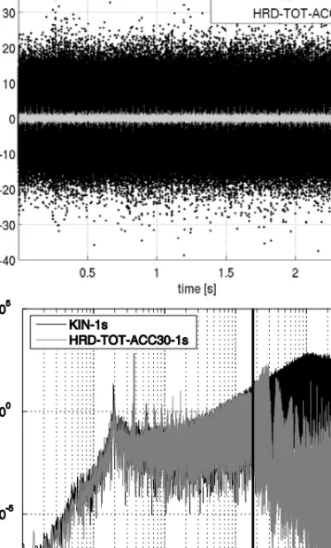
Fig. 1 shows the x-coordinate differences of the solutions ‘KIN’ and ‘ACC30’ with respect to the true orbit for one particular day when both error sources are switched on. The more convenient error characteristics of the HRD positions can be well recognized, as well as the typical variations of the quality of the kinematic positions due to the changing viewing geometry of the GPS satellites seen from the GOCE satellite.

3 . 2 . G r a v i t y F i e l d R e c o v e r y T e s t s

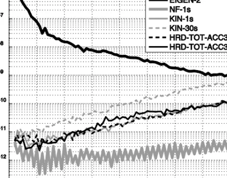
Based on the test scenarios defined in Section 3.1, the energy integral was applied to produce gravity field solutions complete to degree/order 90. The maximum degree n_max = 90 corresponds with the signal content of the input orbits and thus avoids omission errors in the gravity field solutions. The most important results of the gravity field recovery tests are compiled in Fig. 2, and will be discussed in the following subsections.

Table 2. RMS of orbit differences w.r.t. the true orbit.

Orbit Type SIG [mm] NOI [mm] TOT [mm]

KIN 0.5 2.4 2.4 ACC30 0.5 0.5 0.8 ACC60 2.0 0.4 2.1

3 . 2 . 1 . N o i s e - F r e e S c e n a r i o

As a reference configuration, the noise-free orbit ‘NF-1s’ was processed. The grey curve in Fig. 2 shows the deviations from the true gravity field model EIGEN-2 in terms of the degree error median

( ) ( )

median est true

l m Rlm Rlm

σ = ⎧⎨ − ⎫⎬

⎩ ⎭, (10)

Fig. 1. x-coordinate differences with respect to the true orbit for the solutions ‘KIN’ (black) and

‘ACC30’ (grey).

Fig. 2. Deviation from the true gravity field model EIGEN-2 in terms of the degree error median:

where R_lm=

{

C_lm;S_lm

}

are the fully normalized spherical harmonic coefficients, (est) denotes the estimated quantities, and (true) refers to the true gravity field model EIGEN-2.

It can be recognized that the differences are very small, but obviously they are not perfectly noise-free. The residual differences are due to small errors in the orbit data generation (numerical integration), and minor inconsistencies in the GOCE standards implementation at AIUB and TUG. However, the inaccuracies of this reference solution are far below the relevant noise level of the following simulations and do not harm the following interpretations.

3 . 2 . 2 . K i n e m a t i c V e r s u s H R D O r b i t s , 1 - s S a m p l i n g The energy integral was applied to the kinematic orbit ‘KIN-1s’ and the HRD orbit ‘HRD-TOT-ACC30-1s’. The fine grey curve in Fig. 2 shows the degree error median of the solution based on the kinematic orbit, while the dashed black curve displays the result based on the HRD orbit. It can be recognized that the two solutions are very similar. The minor differences in the low degrees can be attributed to the incorrect gravity field information introduced in the ‘HRD-TOT-ACC30-1s’ orbit solution, as it will be shown in Section 3.2.4. Interestingly, a slight improvement of the HRD-solution for the very high degrees, which could have been expected due to the filtering effect of the high-frequency random orbit errors, does not appear in the degree error median plot. An explanation for this behavior is given by the power spectral densities (PSDs) of the residuals of the gravity field adjustment, as it is shown in Fig. 3 (right).

Evidently, the residuals based on the kinematic orbit solution have considerably higher amplitudes in the very high frequency range (black curve), while the filtering effect of the HRD orbit solution (grey curve) in this spectral region can nicely be seen. The vertical line shows the maximum frequency that can be attributed to a gravity field signal complete to degree/order 90. Consequently, the filtering effect acts almost exclusively in the spectral region which is not relevant for a gravity field solution up to degree/order 90. This explains that there are no significant differences between these two solutions for a parameter model complete to degree/order 90. Note that although the residuals of the ‘KIN-1s’ solution have a markedly higher amplitude than those of the ‘HRD-TOT-ACC30-1s’ solution (cf. Fig. 3 left), the quality of the gravity field result is very similar.

Based on the coefficient estimates of the ‘KIN-1s’ and ‘HRD-TOT-ACC30-1s’ solutions, cumulative geoid height errors at degree/order 90 have been computed globally on a 0.5° × 0.5° grid. The standard deviations, evaluated in a latitudinal range of |ϕ| < 83.5° (excluding the polar regions which are not covered by measurements due to the sun-synchronous GOCE orbit), are 8.95 cm for the ‘KIN-1s’ and 8.45 cm for the ‘HRD-TOT-ACC30-1s’ solutions. From these results it can be concluded that the quality of the ‘HRD-TOT-ACC30-1s’ solution is marginally better than the ‘KIN-1s’.

3 . 2 . 3 . K i n e m a t i c V e r s u s H R D O r b i t s , 3 0 - s S a m p l i n g In the case of GOCE precise orbit solutions will be available with a sampling rate of 1 s. Nevertheless, the analysis of less densely sampled input orbits provides valuable insight into the system, because the situation described in Section 3.2.2 changes dramatically when using kinematic and HRD orbits with a sampling interval of 30 s. The

corresponding degree error medians are displayed as grey dashed (kinematic orbit: ‘KIN-30s’) and solid black (HRD orbit: ‘HRD-TOT-ACC30-‘KIN-30s’) curves in Fig. 2. While the 30-s HRD solution is quite similar to the corresponding 1-s solution (and also the result based on the 1-s kinematic orbit), the recovered gravity field model based on the 30-s kinematic orbit solution is markedly degraded.

Fig. 3. Time series of the residual energy (top) and the corresponding PSD (bottom) based on

Due to the fact that the HRD orbits are based on a (reduced-dynamic) force model, they are smoother than the point-wise computed kinematic orbits as shown in Fig. 1. The results of this study clearly underline, however, that compared to the 30-s sampled HRD orbit, the additional observations of the 1-s HRD orbit do not contain additional gravity field information, i.e., the gravity field (complete to degree/order 90) is fully represented by the coarser 30-s sampling.

This, however, is not true for the kinematic orbits, where - due to the point-wise orbit processing and no external force model applied - every data point contains additional gravity field information. This redundancy - and thus the 1-s sampling - is absolutely necessary to achieve a similar performance as in the case of the HRD orbits, because the dominant high-frequency errors (which have been “filtered out” during the HRD orbit processing) can be reduced significantly by additional observations (for the derivation of the velocities from the kinematic orbit position this redundancy is of great help as well). A detailed analysis shows, that the degradation of the 30-s kinematic solution relative to the corresponding 1-s solution follows the statistical √N rule (N being the number of “observations”), i.e., it is about a factor of √30 in the present case.

3 . 2 . 4 . A n a l y s i s o f t h e N o i s e B u d g e t o f t h e H R D O r b i t s In order to analyze the error components of the HRD orbit used in the previous case studies, two additional data sets have been analyzed, including

• only GPS phase noise of 1 mm (‘HRD-NOI-ACC30-1s’);

• only an incorrect gravity field model complete to degree/order 20, zero gravity field coefficients beyond degree/order 20 (‘HRD-SIG-ACC30-1s’).

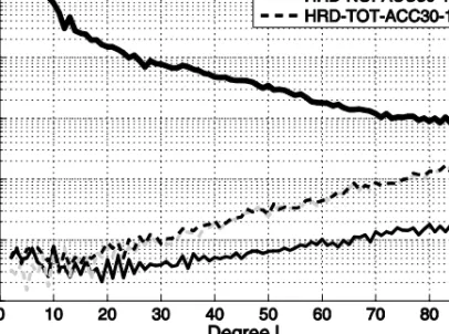
Fig. 4. Deviation from the true gravity field model EIGEN-2 in terms of the degree error median:

Fig. 4 shows the performance of the recovered gravity field model in terms of the degree error median of these two solutions. As a reference, the “sum” of the two effects (‘HRD-TOT-ACC30-1s’) is displayed as dashed curve.

Evidently, the random phase noise (grey curve) dominates the error budget, while the effect of the incorrect a priori gravity field information (black curve) plays only a minor role for the 30 days amount of data. Only at the very low degrees the deviation of the ‘HRD-SIG-ACC30-1s’ solution is slightly larger than the one of the ‘HRD-NOI-ACC30-1s’ solution. This expresses the effect of the incorrect gravity field a priori information up to degree 20 used for the orbit determination. This effect will become more pronounced when analyzing longer data sets due to a further reduction of random errors.

3 . 2 . 5 . T h e E f f e c t o f A P r i o r i G r a v i t y F i e l d I n f o r m a t i o n The HRD orbit is a compromise between a point-wise orbit solution without any a priori gravity field information (kinematic orbit), and the introduction of external (conservative and non-conservative) force models as it is done in the reduced-dynamic processing. In principle the resulting orbit is therefore dependent on the force by which the external information is imposed onto the orbit. In this respect, one of the key parameters of the orbit determination is the time period for the piecewise constant accelerations. A longer period results in a stronger a priori gravity field signal introduced into the orbit solution and vice versa. In all previous simulations, 30-s piecewise constant accelerations have been used. In order to demonstrate the effect of an incorrect gravity field signal on the orbit solution in combination with a too large weight given to this

Fig. 5. Deviations from the true gravity field model EIGEN-2 in terms of the degree error

median. The coefficient estimates are based on HRD orbits with 30-s and 60-s piecewise constant accelerations.

incorrect prior information, the orbits based on 60-s piecewise constant accelerations (‘HRD-TOT-ACC60-1s’) have been analyzed.

The dashed curve in Fig. 5 shows the degree error median of this case study. Compared to the corresponding solution based on the 30-s piecewise constant accelerations (‘HRD-TOT-ACC30-1s’), there is a marked degradation of the solution. Here, the artificially degraded a priori gravity field model, with zero coefficients beyond degree/order 20, considerably degrades the coefficient estimates in this spectral region.

This effect is also evident in the PSD of the residuals of this case study (Fig. 6). Again, the vertical line shows the maximum frequency that can be attributed to a gravity field signal complete to degree/order 90. One clearly sees that firstly, the amplitude of the residual energy of ‘HRD-TOT-ACC60-1s’ is in general higher than the amplitude of ‘HRD-TOT-ACC30-1s’, and secondly, the high-frequency signal component is cut off, leading to a substantially degraded gravity field solution particularly for degrees 35 and higher. In essence, an unbiased recovery of the gravity field from HRD orbit solutions is only possible if the number of stochastic parameters (per component and revolution period of the satellite) is at least equal or greater to twice the maximum degree of the potential to be recovered.

Based on the coefficient estimates of the ‘HRD-TOT-ACC60-1s’ solution, cumulative geoid height errors at degree/order 90 have been computed. The standard deviation of the geoid height errors, evaluated in a latitudinal range of |ϕ| < 83.5°, is 40.8 cm. Compared to the standard deviation of 8.45 cm when using HRD orbits based on 30-s piecewise constant accelerations (see Section 3.2.2), by assigning a too large weight to the

Fig. 6. PSD of residual energy based on HRD orbits with 30-s and 60-s piecewise constant

(incorrect) a priori gravity field information during the HRD orbit processing the resulting gravity field solution is substantially degraded. Much worse results have to expected for this case study when using even longer intervals for the piecewise constant accelerations.

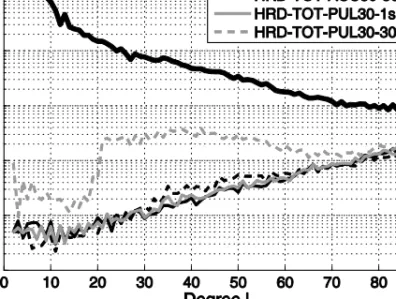
3 . 2 . 6 . P u l s e s v e r s u s P i e c e w i s e C o n s t a n t A c c e l e r a t i o n s The energy integral was also applied to the HRD orbits based on pseudo-stochastic pulses estimated every 30 s. Fig. 7 shows the degree error median of the gravity field recovery based on 1-s TOT-PUL30-1s’) and on 30-s sampled positions (PUL30-30s’), and compares them with the corresponding solutions ‘HRD-TOT-ACC30-1s’ and ‘HRD-TOT-ACC30-30s’ based on piecewise constant accelerations (see Fig. 2). Obviously, both gravity field solutions based on 1-s sampled positions are very similar despite the slightly inferior quality of the pulse-based orbits reported in Section 3.2. The comparison between the recovered gravity field coefficients obtained from the corresponding 30-s sampled positions, however, shows striking differences when using pulse-based instead of acceleration-based orbits. A degradation of almost one order of magnitude can be observed for the solution ‘HRD-TOT-PUL30-30s’ right beyond degree 20, where no a priori information was used for the orbit determination.

Fig. 8 shows the deviations of the pulse-based orbit with respect to the true orbit for a short interval of 10 min. It can be recognized that the maximum deviations occur at the subinterval boundaries every 30 s. Therefore, the striking degradation of the gravity field recovery based on 30-s sampled positions has to be mainly attributed to the special selection of orbit positions at subinterval boundaries. Note that Fig. 8 shows no such boundary effect for the solution based on piecewise constant accelerations, which explains the similar performance of the solutions based on 1-s and 30-s sampled positions in Fig. 7.

4. CONCLUSIONS

From the point of view of gravity field processing with the energy integral approach, the use of HRD orbits has the advantage that orbit velocity information exists, and does not necessarily have to be derived from the orbit positions applying numerical differentiation. Thus, the error component of the numerical differentiation can be avoided. Furthermore our study demonstrates that a less densely sampled orbit (e.g., 30 s instead of 1 s in the present study) based on 30-s piecewise constant accelerations is sufficient to obtain high-quality gravity field solutions, i.e., also the computation time can be reduced significantly. This is due to the fact that HRD orbits have a much more convenient error characteristics and considerably smaller noise amplitudes predominantly in the high-frequency region.

On the other hand, the main advantage of kinematic orbits is that they are not based on external force models for the LEO orbit determination. The deteriorating effect of incorrect prior information was demonstrated in Sections 3.2.5 and 3.2.6. Therefore, it can be concluded, that great care has to be taken for the choice of the a priori model which is “impressed” onto the HRD orbit solution. In principle, the whole bandwidth between the “extreme” cases, the kinematic orbit on the one hand, and a fully dynamic orbit on the other hand, can be realized. An unbiased recovery of the gravity field from HRD orbit solutions is, however, only possible if the number of stochastic parameters (per

component and revolution period of the satellite) is at least equal or greater to twice the maximum degree of the potential to be recovered.

We also demonstrated that a comparable gravity field accuracy as for HRD orbit solutions can be obtained from kinematic orbits, if the complete numerical “arsenal” (high redundancy of 1-s orbit sampling, high-performance numerical differentiation techniques to derive velocity information, etc.) is used, but at the price of higher CPU requirements.

The transition from the purely kinematic to the HRD orbit type can be considered as a low-pass filter procedure, i.e., improvements in the gravity field solution due to the application of HRD orbits are first to be expected in the higher degrees of the harmonic spectrum (due to the smoothing of high-frequency orbit errors), while the lower degrees remain practically unaltered. Considering the final goal of an optimum combined GOCE

Fig. 7. Deviations from the true gravity field model EIGEN-2 in terms of the degree error

median. The coefficient estimates are based on HRD orbits (1 s and 30 s sampled) with piecewise constant accelerations and pulses, respectively.

Fig. 8. x-coordinate differences with respect to the true orbit for the solutions ‘PUL30’ (black)

gravity field solution from SST-hl and satellite gravity gradiometry (SGG), the largest benefit using HRD orbits appears in the higher degrees of the harmonic spectrum. This, however, should anyway be captured by the SGG component almost exclusively, i.e., the benefit of the use of HRD orbits for a combined gravity solution seems to be very small.

If it is the goal to produce a combined GOCE-only gravity field solution, i.e., ideally without using any external gravity field information, the kinematic orbit type has to be favored. The price to be paid then is the use of kinematic orbits with less convenient error characteristics and higher noise amplitudes.

Acknowledgements: This study was performed in the framework of the ESA Project GOCE High-Level Processing Facility (Main Contract No. 18308/04/NL/MM).

References

Badura T., 2006. Gravity Field Analysis from Satellite Orbit Information applying the Energy Integral Approach. PhD Thesis, Graz University of Technology, Graz, Austria.

Badura T., Sakulin C., Gruber C. and Klostius R., 2006. Derivation of the CHAMP-only global gravity field model TUG-CHAMP04 applying the energy integral approach. Stud. Geophys. Geod., 50, 59−74.

Beutler G., 2005. Methods of Celestial Mechanics. Springer, Berlin.

Beutler G., Jäggi A., Hugentobler U. and Mervart L., 2006. Efficient satellite orbit modelling using pseudo-stochastic parameters. J. Geodesy, 80, 353−372.

Bock H., Jäggi A., Švehla D., Beutler G., Hugentobler U. and Visser P., 2007. Precise orbit determination for the GOCE satellite using GPS. Adv. Space Res., 39, 1638−1647.

Dach R., Hugentobler U., Fridez P. and Meindl M. (Eds.), 2007. Bernese GPS Software Version 5.0. Astronomical Institute, University of Bern, Bern, Switzerland.

Ditmar P., Kuznetsov V., van Eck van der Sluijs A.A., Schrama E. and Klees R., 2006. ‘DEOS_CHAMP-01C_70’: a model of the Earth’s gravity field computed from accelerations of the CHAMP satellite. J. Geodesy, 79, 586−601.

ESA, 1999. Gravity Field and Steady-State Ocean Circulation Explorer Mission. Reports for Mission Selection. The Four Candidate Earth Explorer Core Missions, SP-1233(1), European Space Agency, Noordwijk, The Netherlands.

Földváry L., Švehla D., Gerlach C., Wermuth M., Gruber T., Rummel R., Rothacher M., Frommknecht B., Peters T. and Steigenberger P., 2004. Gravity model TUM-2Sp based on the energy balance approach and kinematic CHAMP orbits. In: Reigber C., Lühr H., Schwintzer P. and Wickert J. (Eds.), Earth Observation with CHAMP - Results from Three Years in Orbit, Springer Verlag, Heidelberg, Berlin, New York, 13−18.

Gerlach C., Földváry L., Švehla D., Gruber T., Wermuth M., Sneeuw N., Frommknecht B., Oberndorfer H., Peters T., Rothacher M., Rummel R. and Steigenberger P., 2003. A CHAMP-only gravity field model from kinematic orbits using the energy integral. Geophys. Res. Lett.,

30, Art.No.2037.

Goiginger H. and Pail R., 2007. Investigation of velocities derived from satellite positions in the framework of the energy integral approach. In: Fletcher K. (Ed.), Proceedings of the 3rd

International GOCE User Workshop, ESA Special Publication SP-627, ISBN 92-9092-938-3, European Space Agency, Noordwijk, The Netherlands, 319−324.

GRACE, 1998. Gravity Recovery and Climate Experiment: Science and Mission Requirements Document. Revision A. JPLD-15928, NASA’s Earth System Science Pathfinder Program, Jet Propulsion Laboratory, Pasadena, CA.

Ilk K.-H., 2002. Energy relations for the motion of two satellites within the gravity field of the Earth. In: Sideris M.G. (Ed.), Gravity, Geoid and Geodynamics 2000. International Association of Geodesy Symposia, 123, Springer-Verlag, Berlin, 129−135.

Jäggi A., Hugentobler U. and Beutler G., 2005. Efficient stochastic orbit modeling techniques using leaast squares estimators. In: Sansò F. (Ed.), A Window on the Future of Geodesy. International Association of Geodesy Symposia, 128, Springer-Verlag, Berlin, 175−180. Jäggi A., 2006. Pseudo-Stochastic Orbit Modeling of Low Earth Satellites Using the Global

Positioning System. PhD Thesis, Astronomical Institute, University of Bern, Bern, Switzerland.

Jäggi A., Beutler G., Bock H. and Hugentobler U., 2007. Kinematic and highly reduced-dynamic LEO orbit determination for gravity field estimation. In: Tregoning P. and Rizos C. (Eds.), Dynamic Planet - Monitoring and Understanding a Dynamic Planet with Geodetic and Oceanographic Tools. International Association of Geodesy Symposia, 130, Springer-Verlag, Berlin, 354−361.

Jekeli C., 1999. The determination of gravitational potential differences from satellite-to-satellite tracking. Celest. Mech. Dyn. Astron., 75, 85−101.

Montenbruck O. and Gill E., 2000. Satellite Orbits - Models, Methods and Applications. Springer-Verlag, Berlin, Germany.

O’Keefe J.A., 1957. An application of Jacobi’s integral to the motion of an Earth satellite. Astron. J., 62, 265-266.

Mayer-Gürr T., Ilk K.H., Eicker A. and Feuchtinger M., 2005. ITG-CHAMP01: a CHAMP gravity field model from short kinematic arcs over a one-year observation period. J. Geodesy, 78, 462−480.

Migliaccio R., Reguzzoni M. and Sansó F., 2003. Spacewise approach to satellite gravity field determination in the presence of coloured noise. J. Geodesy, 78, 304−313.

Pail R., Metzler B., Preimesberger T., Goiginger H., Mayrhofer R., Höck E., Schuh W.-D., Alkathib H., Boxhammer C., Siemes C. and Wermuth M., 2007. GOCE-Schwerefeldprozessierung: Software-Architektur und Simulationsergebnisse. Zeitschrift für Geodäsie, Geoinformation und Landmanagement, Heft 1/2007, Deutscher Verein f. Vermessungswesen e.V., 16−25. Prange L., Jäggi A., Beutler G., Mervart L. and Dach R., 2008. Gravity field determination at the

AIUB - the celestial mechanics approach. In: International Association of Geodesy Symposia, Springer-Verlag, Berlin (in print).

Reigber C., Schwintzer P. and Lühr H., 1999. CHAMP geopotential mission. Boll. Geof. Teor. Appl., 40, 285−289.

Reigber C., Schwintzer P., Neumayer K.-H., Barthelmes F., König R., Förste C., Balmino G., Biancale R., Lemoine J.-M., Loyer S., Bruinsma S., Perosanz F. and Fayard T., 2007. The CHAMP-only Earth gravity field model EIGEN-2. Adv. Space Res., 31, 1883−1888.

Rummel R., Gruber T. and Koop R., 2004. High level processing facility for GOCE: products and processing strategy. GOCE, the Geoid and Oceanography, Proceedings of the 2nd International GOCE User Workshop. ESA Special Publication SP-569, ISBN 92-9092-880-8, European Space Agency, Noordwijk, The Netherlands.

Švehla D. and Rothacher M., 2002. Kinematic and reduced-dynamic precise orbit determination of low Earth orbiters. Adv. Geosci., 1, 47−56.

Wu S.C., Yunck T.P. and Thornton C.L., 1991. Reduced-dynamic technique for precise orbit determination of low Earth satellites. J. Guid. Control Dyn., 14, 24−30.

Visser P.N.A.M., Sneeuw N. and Gerlach C., 2003. Energy integral method for gravity field determination from satellite orbit coordinates. J. Geodesy, 77, 207−216.