Identifying factors limiting legume biomass production in a heterogeneous on-farm environment

(1)

CROPS AND SOILS RESEARCH PAPER

Identifying factors limiting legume biomass production in a

heterogeneous on-farm environment

S. DOUXCHAMPS1*, E. FROSSARD1, N. UEHLINGER1, I. RAO2, R. VAN DER HOEK3, M. MENA4,

A. SCHMIDT3 AN DA. OBERSON1

1

ETH Zurich, Institute of Agricultural Sciences, Eschikon 33, 8315 Lindau, Switzerland 2_{Centro Internacional de Agricultura Tropical (CIAT), A.A. 6713, Cali, Colombia} 3

Centro Internacional de Agricultura Tropical (CIAT-Central America), Apartado Postal LM-172, Managua, Nicaragua 4_{Instituto Nicaragüense de Tecnología Agropecuaria (INTA), Managua, Nicaragua}

(Received 14 July 2011; revised 17 October 2011; accepted 23 November 2011; first published online 4 January 2012)

SUMMARY

Multipurpose legumes provide a wide range of benefits to smallholder production systems in the tropics. The degree of system improvement after legume introduction depends largely on legume biomass production, which in turn depends on the legumes’ adaptation to environmental conditions. For Canavalia brasiliensis (canavalia), an herbaceous legume that has been recently introduced in the Nicaraguan hillsides, different approaches were tested to define the biophysical factors limiting biomass production on-farm, by combining information from topsoil chemical and physical properties, topography and soil profiles.

Canavalia was planted in rotation with maize during two successive years on 72 plots distributed over six farms and at contrasting landscape positions. Above-ground biomass production was similar for both years and varied from 448 to 5357 kg/ha, with an average of 2117 kg/ha. Topsoil properties, mainly mineral nitrogen (N; ranging

25–142 mg/kg), total N (Ntot; 415–2967 mg/kg), soil organic carbon (SOC; 3–38 g/kg) and pH (5·3–7·1),

significantly affected canavalia biomass production but explained only 0·45 of the variation. Topography alone explained 0·32 of the variation in canavalia biomass production. According to soil profiles descriptions, the best production was obtained on profiles with a root aggregation index close to randomness, i.e. with no major obstacles for root growth. When information from topsoil properties, topography and soil profiles was combined through a stepwise multiple regression, the model explained 0·61 of the variation in canavalia biomass (P < 0·001) and included soil depth (0·5–1·70 m), slope position, amount of clay (19–696 kg/m2) and stones (7–727 kg/m2) in the whole profile, and SOC and N content in the topsoil. The linkages between topsoil properties, topography and soil profiles were further evaluated through a principal component analysis (PCA) to define the best landscape position for canavalia cultivation.

The three data sets generated and used in the present study were found to be complementary. The profile description demonstrated that studies documenting heterogeneity in soil fertility should also consider deeper soil layers, especially for deep-rooted plants such as canavalia. The combination of chemical and physical soil properties with soil profile and topographic properties resulted in a holistic understanding of soil fertility heterogeneity and shows that a landscape perspective must be considered when assessing the expected benefits from multipurpose legumes in hillside environments.

INTRODUCTION

The use of multipurpose legumes has been promoted to increase the productivity and the resilience of

smallholder systems in the tropics (Giller2001; Cherr et al.2006). Benefits reported for cropped soils are the addition of nitrogen (N) via symbiotic N2fixation, the build-up of soil organic matter stocks, reduction of run-off and soil erosion and the enhancement of quan-tity and quality of crop residues that are fed to livestock

* To whom all correspondence should be addressed. Email: s.douxchamps@cgiar.org

Journal of Agricultural Science(2012), 150, 675–690. © Cambridge University Press 2012 doi:10.1017/S0021859611000931

https:/www.cambridge.org/core/terms. https://doi.org/10.1017/S0021859611000931

(2)

(Said & Tolera 1993; Boddey et al. 1997; Giller 2001; Pansak et al. 2008). Legume performance in providing those benefits depends largely on biomass production. N2 fixation and N uptake were reported as being proportional to legume biomass production

(Douxchamps et al. 2010; Unkovich et al. 2010).

Economic benefits from legumes are also directly linked to legume productivity (Ebanyat et al.2010).

The general degree of system improvement therefore depends on legume biomass production, which in turn depends on the legume adaptation to climate and soil fertility conditions. It is common for soil conditions to be highly heterogeneous in most low input smallholder farming systems (Tittonell et al.

2005; Zingore et al. 2007), and legumes must be

targeted to locations where only a few factors limit

biomass production (Ojiem et al. 2007). Numerous

constraints determine soil fertility in hillside environ-ments (de Costa & Sangakkara 2006) and the issue must be addressed within a landscape perspective, as biomass production is very much affected by land-scape position (Kravchenko et al. 2000; Iqbal et al. 2005; Thelemann et al.2010).

Often, a rich database on the adaptation of legumes to soil types is available for well-known legumes. However, for new legume options, very limited in-formation is available and there is no consensus on how to assess the environmental factors systematically (i.e. soil properties and topography) limiting biomass production for new varieties.

Biomass studies are based either on soil chemical and/or physical properties (Daellenbach et al.2005; Ojiem et al. 2007; Ebanyat et al. 2010) or on topo-graphy (Guretzky et al.2004; Thelemann et al.2010), or both (Kravchenko et al.2000; Iqbal et al.2005). To the knowledge of the present authors, topsoil proper-ties, topography and soil profile description have never been combined in a single biomass study.

In 2007, the tropical multipurpose legume

Canavalia brasiliensisMart. Ex. Benth (canavalia) was introduced into the smallholder crop–livestock system of the Nicaraguan hillsides with the purpose of restoring and maintaining soil fertility of cropping areas and increasing the availability of dry season feed for livestock. The main objectives of the present study were to: (i) identify the factors limiting on-farm biomass production of canavalia by combining information from soil profiles, topsoil properties and topography; and (ii) define the best landscape position for

in-troducing canavalia for improved crop–livestock

production.

MATERIALS A ND METHODS Sites and field experiments

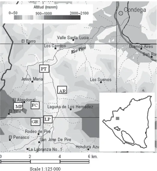
The study area is located in the Rio Pire watershed (Department of Estelí, northwestern Nicaragua), within a 2 km radius around the community of Santa Teresa

(13°18′N, 86°26′W, 600–900 m a.s.l.). Soils are

classified as Udic and Pachic Argiustolls (Suppl Mat 1). The climate is classified as tropical savannah according to the Köppen–Geiger classification (Peel et al. 2007). Annual mean rainfall (since 1977) is 825 mm (INETER2009) and has a bimodal distribution

pattern between June–August and September–

November. Six farmers from Santa Teresa who were interested in integrating canavalia on a part of their cropped land were identified. They chose the exper-imental sites within their farms themselves; these were named after the farmer’s initials. The sites presented a range of topographical features with varying soil characteristics, representative of the cropping area environmental conditions of the Rio Pire watershed

(Fig. 1). Three sites were located in the bottom of the

valley (PT, AR and LP), two at a medium level (GR and FC) and one on the top of the hill (MP). All sites were part of the same slope with eastern exposure except site AR, which was situated in front on the western exposed slope. Sites AR and GR showed high topographic variability within-site, as they were located on irregular small hills and depressions. Sites MP and FC were located on irregular slopes. Sites LP and PT were flat with homogeneous topography.

Farmers were traditional crop–livestock small-holders, cultivating maize and beans on c. 2 ha of land and grazing their cattle on communal pastures based on Jaragua grass (Hyparrhenia rufa (Nees) Stapf.). Cultivation is carried out essentially with hand-held tools. Prior to sowing maize, land is usually prepared with a plough pulled by oxen if accessibility to the field and slopes allow; otherwise it is prepared manually using a hoe. Maize is sown at the end of May, at the onset of the first rainy season. Maize is fertilized with urea (80 kg/ha on average) 8 days after sowing, sometimes complemented with compound fertilizer (120 g N/kg, 300 g P2O5/kg and 100 g K2O/kg) at fertilizer amounts up to 96 kg/ha, in one dose 22 days after sowing. At maturity, plants are cut above the ears and maize ears are left drying on the

stalks for 2–3 months. Meanwhile, common beans

are sown around mid-September between the maize rows, to take advantage of this part of the bimodal rainfall pattern. Maize and beans are both harvested in

(3)

December. In January, at the beginning of the dry season, forage becomes scarce in the grazing areas and farmers let their cattle enter the cultivated fields to graze on crop residues.

Trials aiming at comparing the N budget of the traditional maize–bean rotation (1st rainy season–2nd rainy season) with an alternative maize–canavalia rotation were established on all sites. Full details of the design, relevance of the proposed rotation for small-holder crop–livestock farmers and resulting N budgets are reported in Douxchamps et al. (2010). Since the aim of the present study was to identify factors influencing the high variability in canavalia biomass production observed in these trials, only the plots with maize–canavalia rotation are considered here. In brief, four 100 m2 plots of maize–canavalia rotation were repeated in three completely randomized blocks at each site, resulting in 12 plots per site and a total

of 72 plots on six farms. At the end of September 2007, weeds were cut with large knives (machetes) and canavalia (CIAT 17009) was sown with a stick between maize rows with a row-to-row spacing of 0·5 m and a plant-to-plant spacing of 0·2 m. No fertilizer was applied to canavalia. At the end of January 2008, four different proportions of canavalia above-ground bio-mass were removed from the four plots in each block to simulate different grazing rates for the N budget experiment (Douxchamps et al. 2010). In June 2008, the remaining biomass of canavalia was cut before planting maize and the plots were managed the same way as in 2007, with canavalia sown at the end of September 2008 between the maize rows and cut 4 months later at the end of January 2009. Precipitation during canavalia growth (September– January) was 540 mm in 2007 and 460 mm in 2008, which was above the normal rainfall in the region. Fig. 1. Location of the sites in the Rio Pire watershed (source: MAGFOR, see Suppl Mat 1). The map inserted at the bottom right depicts Nicaragua, the grey square being the study area.

Factors limiting legume biomass production on-farm 677

(4)

Temperatures for both years were similar, with a mean of 23 °C, a maximum of 32 °C and a minimum of 14 °C (INETER2009).

Biomass production of canavalia

Before cutting canavalia in January 2008 and 2009, above-ground biomass production and soil cover were determined in each plot with the comparative yield method (Haydock & Shaw1975), in which the yields from 1 m2quadrats placed at random were rated with respect to a set of five reference preselected quadrats that provided a scale covering the range of biomass encountered within each plot. This method was chosen because biomass production needed to be evaluated without being harvested, for the purpose of the N budget experiment.

Environmental factors

Topsoil chemical and physical characteristics

In September 2007, topsoil (0–100 mm) was collected with a soil corer in each plot (12 cores per plot), bulked together to form a composite sample per plot, air-dried, sieved at 2 mm and brought to the CIAT laboratories in Cali, Colombia. Samples were analysed for soil organic carbon (SOC) by K2Cr2O7 oxidation

(Nelson & Sommers 1982), total N (Ntot) by a

modification of the Berthelot reaction (Krom 1980), available phosphorus (P) using anion exchange resins (Tiessen & Moir1993), total P (Ptot) by acid digestion (Olsen & Sommers 1982), pHH2O in a soil-water suspension (Salinas & Garcia1985), cation exchange

capacity by NH4+ saturation (Mackean 1993) and

mineral N by 1M KCl (Anderson & Ingram 1993).

The same sampling was repeated in October 2008

and samples were again analysed for mineral N. A mean of the mineral N data of both years was used for the subsequent statistical analysis.

Soil physical properties of the topsoil (0–100 mm) of four contrasting sites (PT, GR, LP and MP; two plots per block) were determined in the soil physics laboratory of CIAT. An unsieved soil sample was used for the determination of aggregate stability (Yoder1936) with an apparatus similar to that described by Bourget & Kemp (1957). Three undisturbed soil cores of 50 mm of diameter per 50 mm length were taken per plot and analysed for water retention (Richards & Weaver 1944), bulk density and texture (Bouyoucos1962). Topography

Slope angle was measured on three representative points in each plot using an A mason level. Slope position was defined for each plot according to the five-unit model of Ruhe & Walker (1968) and included summit, upper slope, mid slope, lower slope and bottom positions. As in most of the studies applying this model (Iqbal et al. 2005), the boundary lines between position types were arbitrary. The topo-graphic description of the plots was completed for each plot by the hill form (convex, straight or concave). Soil profiles and rooting patterns

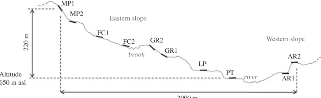
Ten groups of plots with common properties were defined based on chemical and topographic proper-ties, i.e. on all properties measured at single plot level, using an ordination plot (Anderson2004). Each group corresponded to a distinct landscape position (Fig. 2). In the second year, 4 months after canavalia establish-ment, one soil profile was opened for each group, at a 0·15 m distance parallel to plant rows, on a length

220 m MP1 MP2 FC1 FC2 GR2 ~3000 m GR1 LP PT river AR2 Western slope AR1 brook Eastern slope Altitude 650 m asl

Fig. 2. Transversal view of the landscape positions of the profiles. MP1, upland, hillslope; MP2, upland, terrace; FC1, upland, smooth slope; FC2, upland, brookside; GR2, hillslope shoulder; GR1, hillslope foot; LP, lowland, terrace; PT, floodplain; AR1, depositional area; AR2, summit.

(5)

of c. 1·20 m. Profiles were as deep as permitted by soil hardness. Profiles were named after the site in which they were examined. Detailed profile descriptions included sketch maps, horizon identification (Brady & Weil2007), soil colour, structure and fractions, as well as maps of rooting patterns. Soil colour was defined following a standard colour chart (Oyama & Takehara 1967). Soil fractions (i.e. proportions of clay, silt, sand, gravel and stones) were determined visually in the field according to the diameter ranges of Kuntze et al. (1981). Stones were defined as soil particles with a diameter >60 mm. The weight of stones, clay, silt and sand per profile was calculated from the fraction percentage of each horizon and an estimation of its bulk density following Brady & Weil (2007). The amount of each fraction per profile was the sum of the amounts in each horizon. The amount of fine earth per profile was the sum of the amounts of clay, silt and sand. A transparent plastic sheet was placed on the wall of the profile and positions of visible root contacts were marked with a pen (Tardieu1988). All living roots were attributed to canavalia plants, as there were no other plant species in the soil surrounding the profile. The resulting point patterns were then digitalized. Roots were made visible up to the plant line using small knives, and sketched. Lateral roots, which are known to be extended for canavalia (Alvarenga et al. 1995), were not included in the sketches as their excavation was not feasible in the present trial.

Statistical analysis

Statistical analyses were performed using the program

R (R Development Core Team 2007). Data from the

profiles were assigned to all plots from the own profile group. For soil physical properties, which were not defined for all plots (see above, topsoil chemical and physical characteristics), average values from their own group were imputed for missing values. First, each type of data (profiles, topographic properties and topsoil properties) was analysed separately. Then, the three types of data were combined and analysed using multivariate statistics.

Canavalia

Canavalia data were submitted to a Wilcoxon rank-sum test to check for significant differences between the 2 years. The significance of the effect of the cut of 2007 on the performance of 2008 was tested by an analysis of variance (ANOVA) using the aov function

in R (Chambers et al. 1992). The model contained

treatment as fixed factor, site and block as random factors, with block being nested within site. The significance level chosen was P = 0·05.

Topsoil data

The topsoil properties influencing canavalia biomass production were selected with a stepwise multiple regression, using the function lme in R (Pinheiro & Bates2000).

Topographic data

The proportion of variability in canavalia biomass production explained by topographic properties was determined with a multiple regression, using the function lm in R (Pinheiro & Bates2000). Categorical variables were fitted by set.

Profile data

In the profiles, root aggregation index and intensity of soil exploration by roots were determined by analysing root point patterns using the package spatstat in R (Baddeley & Turner 2005). The root aggregation index is measured based on the nearest neighbour distance, and indicates the degree of randomness in the spatial root distribution pattern. It takes values from 0 to 2, with 0 indicating the maximum degree of clustering, 1 indicating a random pattern and 2 indicating a uniform pattern (Baddeley & Turner

2005).

Combination of the three data sets

First, the environmental factors (i.e. topsoil, profile and topographic variables) influencing canavalia biomass production were selected with a stepwise multiple regression, using the function lme in R (Pinheiro & Bates 2000). Right-skewed variables were log-transformed before the regression. Model simpli-fication was done using stepAIC in R (Venables &

Ripley 2002), which uses the Aikake information

criterion (AIC) as automated selection tool according to maximum likelihood. The significance level chosen was P = 0·05.

Second, the principal component analysis (PCA) was used to link environmental properties to land-scape positions from the profile groups. The PCA was performed using princomp in R (Mardia et al.1979). Variables were scaled and standardized before the PCA.

(6)

RESULTS

Biomass production of canavalia

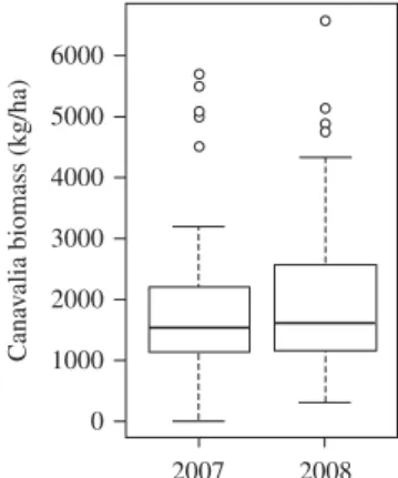
Canavalia above-ground biomass production per plot varied from 0 to 5700 kg/ha in 2007 and from 290 to 6570 kg/ha in 2008 (Fig. 3). It did not significantly differ between 2007 and 2008 (P = 0·740). The biomass removal treatments applied when cutting canavalia at the end of the growing season 2007 had no significant effect on the production in 2008 (P = 0·407). Therefore, for each plot, mean values of both years were used in the subsequent analysis. Within-site variation ranged from 0·25 (LP site) to 0·70 (AR site), whereas variation between sites was 0·32. Soil cover by canavalia varied from 0·13 to 0·96 of the soil surface, with a mean value of 0·53. It was positively correlated with canavalia biomass (cover (%) = 30 Ln (biomass (kg/ha))–171; R2= 0·78). An increase in biomass up to 3000 kg/ha also induced an important increase in soil cover, whereas beyond this yield the cover increased by only c. 0·05 for an increase of 1000 kg/ha biomass. Cover was not included in the multiple regression analysis because it was highly correlated with canavalia biomass production.

Topsoil properties

The ranges of values taken by the topsoil variables and their median are presented inTable 1. All quantitative variables except for water retention and pH took a broad range of values. In the plots, topsoil had no extreme pH values, indicating slightly acid to neutral

soils. SOC ranged from 3 to 38 g/kg, and Ntot ranged from 415 to 2967 mg/kg. The median available P was 24 mg/kg.

The regression on the topsoil data showed that Ntot, bulk density, pH, SOC and Nmin affected significantly canavalia biomass production (P = 0·003, 0·004, 0·007, 0·010 and 0·010, respectively), and explained 0·45 of the variation in canavalia biomass production.

Topographic properties

The ranges of values observed for the topographic variables are presented in Table 1. About 0·39 of the plots had slope angle of more than 11°. Most of the plots (0·78) had a straight slope form. Few plots (0·06) were located on a local summit, whereas 0·64 of the plots were on the lower part (0·23) or the bottom of the slopes (0·41). In the profiles, the amount of stones ranged from 7 to 727 kg/m2, whereas the amount of fine earth (i.e. all particles finer than 2 mm) ranged from 175 to 2328 kg/m2. The amount of fine earth per profile was highly correlated with depth (R2= 0·89).

The regression on topographic data only showed that topographic variables explained a significant proportion of the variation in canavalia biomass (0·32, P = 0·001), with slope position as main factor.

Soil profiles and rooting patterns

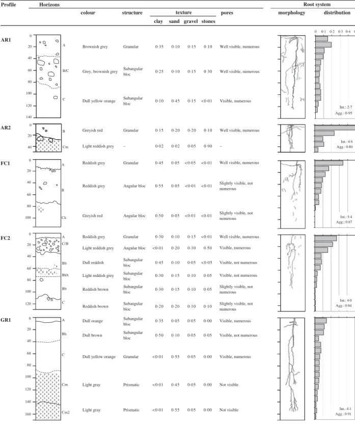
Description of soil profiles is presented inTable 2. The topsoil and topographic characteristics of the plots where profiles were made are presented in Table 3. Profiles on lower slope or bottom positions were deeper than profiles located on upper slope or summit positions. Stony or compacted layers affected root morphology. More than 0·20 of roots were counted in the first 0·2 m soil depth in the profiles with high amounts of organic matter as well as in the profiles where a stony layer hindered root growth. The root aggregation index for all profiles was between 0·6 and 1.

The biomass production of canavalia associated with each profile group is shown inFig. 4. A one-way ANOVA showed that there were significant differences between the mean canavalia biomass production per profile group (P < 0·001).

Combination of the three data sets

Results of the stepwise multiple regression indicated that the variables retained after the model reduction

6000 5000 4000 3000 2000 1000 Cana v

alia biomass (kg/ha)

0

2007 2008

Fig. 3. Canavalia above-ground biomass production on all sites in 2007 and 2008. The ends of the boxes are the upper and lower quartiles, the horizontal bold lines are the medians, the vertical lines are the full range of values, and the dots are outliers.

(7)

Table 1. Overview of the variable used in the statistical analyses

Set Abbreviation Variable Variable type Definition Units

Range or proportion

of total* (n = 69) Median

Farm Plough Use of plough Categorical Field n.a. 0·67 n.a.

Chemical properties† pH pH Quantitative Plot n.a. 5·3–7·1 6·4

CEC Cation exchange capacity Quantitative Plot mmol/kg 266–518 362

Ntot Soil total N Quantitative Plot mg/kg 415–2967 1552

Nmin Soil mineral N Quantitative Plot mg/kg 25–142 59

SOC Soil organic carbon Quantitative Plot g/kg 3–38 21

Ptot Soil total phosphorus Quantitative Plot mg/kg 122–730 464

Presin Soil available phosphorus Quantitative Plot mg/kg 6–86 24

Physical properties† WSA Water stable aggregates (> 0·25 mm) Quantitative Plot or profile group g/g 0·21–0·73 0·40

UA Unstable aggregates (< 0·125 mm) Quantitative Plot or profile group g/g 0·21–0·63 0·47

ρ Bulk density Quantitative Plot or profile group Mg/m3 0·97–1·40 1·18

θFC Water content at field capacity Quantitative Plot or profile group m3/m3 0·35–0·45 0·40

θWP Water content at wilting point Quantitative Plot or profile group m3/m3 0·24–0·38 0·32

Porosity Porosity Quantitative Plot or profile group m3/m3 0·47–0·62 0·56

Slope angle Slope Slope angle Quantitative Plot ° 0–26·1 4·6

Slope form Straight Straight slope Categorical Plot n.a. 0·78 n.a.

Concave Slope with concave form Categorical Plot n.a. 0·12 n.a.

Slope position Summit Plot on the summit of local hill Categorical Plot n.a. 0·06 n.a.

Upperslope Plot on upper part of slope Categorical Plot n.a. 0·09 n.a.

Lowerslope Plot on lower part of slope Categorical Plot n.a. 0·23 n.a.

Bottom Plot on the bottom of local hill Categorical Plot n.a. 0·41 n.a.

Depth Depth Depth of the profile Quantitative Profile group m 0·50–1·70 1·18

Texture‡ Clay Amount of clay Quantitative Profile group kg/m2profile 19–696 448

Stone Amount of stones Quantitative Profile group kg/m2_profile _7–727 ₂₉₇

* Range is given for quantitative variables and proportion of total is given for categorical variables. † Properties measured in the topsoil (0–0·1 m).

‡ Properties measured on the whole profile, for a volume of 1 m2

× profile depth. n.a. = non applicable.

Fa ctors limiting legume bioma ss production on-farm 681 https:/www.cambridge.org/core/terms . https://doi.org/10.1017/S0021859611000931 Downloaded from https:/www.cambridge.org/core

. University of Basel Library

, on

30 May 2017 at 21:22:52

(8)

Table 2. Profiles description, including horizons identification, soil colour, structure and fractions, as well as rooting patterns. Root distribution is the number of root points per depth, in proportion of total. Intensity (Int., number of root points/dm2) and aggregation index (Agg.) are given in the bottom right of each root

distribution profile Profile Horizons distribution morphology pores e r u t c u r t s r u o l o c

clay sand gravel stones texture Root system Int.: 2·7 Agg.: 0·95 Int.: 4·6 Agg.: 0·80 Int.: 4·0 Agg.: 0·84 Int.: 5·4 Agg.: 0·87 Int.: 4·1 Agg.: 0·91 0 20 40 60 80 100 120 140 0 20 40 A B/C C B Cm AR1 AR2 0 20 40 60 80 100 0 20 40 60 80 100 120 A C/B Bb Bkb Bb C A B Ck FC1 FC2 0 20 40 60 80 100 120 140 160 A Bh C Cm Cm2 GR1

Brownish grey Granular 0·35 0·10 0·15 0·10 Well visible, numerous

Grey, brownish grey Subangular

bloc 0·25 0·10 0·15 0·30 Well visible, numerous

Dull yellow orange Subangular

bloc 0·10 0·45 0·15 <0·01 Visible, numerous

Greyish red Granular 0·15 0·20 0·20 0·10 Well visible, numerous

Light reddish grey – 0·02 0·02 0·05 0·90 –

Reddish grey Granular 0·45 0·05 <0·05 <0·01

Reddish grey Angular bloc 0·55 0·05 <0·01 <0·01

Greyish red Angular bloc 0·50 0·05 <0·01 <0·01

Reddish grey Granular 0·30 0·10 0·15 <0·01 Light reddish grey Angular bloc <0·01 0·20 0·30 0·50

Dull reddish Subangular

bloc 0·45 0·10 0·05 <0·05 Light reddish grey Subangular

bloc 0·30 0·15 0·10 0·05

Reddish brown Subangular

bloc 0·30 0·15 0·10 0·05

Reddish brown Subangular

bloc 0·20 0·20 0·10 0·10

Slightly visible, not numerous Well visible, numerous Visible, numerous

Visible, not numerous Well visible, numerous

Slightly visible, not numerous

Visible, not numerous Slightly visible, not numerous

Dull orange Subangular

bloc 0·35 0·05 0·05 0·00 Visible, numerous Dull brown Subangular

bloc 0·50 0·10 0·05 0·05 Visible, not numerous

Dull yellow orange Granular <0·01 0·55 0·05 0·00 Visible, numerous

Light gray Prismatic <0·01 0·45 0·05 0·00 Not visible

Light gray Prismatic <0·01 0·55 0·05 0·00 Not visible

(9)

Table 2. (Continued) Int.: 2·8 Agg.: 0·72 Int.: 4·7 Agg.: 0·68 Int.: 5·2 Agg.: 0·80 Int.: 3·5 Agg.: 0·93 Int.: 3·2 Agg.: 0·84

Organic material slightly decomposed White colour

Compacted / dense material Mineral concretions

Stones

Abrupt / clear / sharp separation Gradual / diffuse separation 0 20 40 60 80 100 120 140 A Bkv Btg C GR2 0 20 40 60 80 100 120 140 Ap B C Cm C Cb CBm LP OA C/Bh Bk 0 20 40 60 80 100 0 20 40 60 80 A Bh Bk C MP2 MP1 PT 0 20 40 60 80 100 Ae A Bc Bt B

Light yellow Subangular

bloc 0·05 0·70 0·10 <0·01 Visible

Light grey Prismatic <0·01 0·60 <0·01 <0·01 Visible, not numerous

Yellowish Prismatic <0·01 0·65 0·05 0·01 Not visible

Dull yellow orange Prismatic <0·01 0·80 0·10 <0·01 Visible, not numerous

Profile Horizons

distribution pores

structure colour

clay sand gravel stones texture

Root system

Light reddish grey Granular 0·20 0·25 0·05 0·00 Well visible, numerous Reddish grey Subangular

bloc 0·15 0·20 0·10 0·05 Well visible, numerous Light reddish grey – 0·05 0·10 0·25 0·60 –

Reddish grey Compacted 0·05 0·60 0·05 <0·05 – Light reddish grey – <0·05 0·10 0·20 0·70 –

Reddish grey Granular 0·00 0·90 0·05 <0·01 –

Greyish Compacted 0·60 0·05 0·00 <0 ·10 –

Reddish grey Granular 0·25 0·05 0·15 0·10 Visible, numerous Dark reddish Subangular

bloc 0·40 0·05 0·15 0·10 Well visible, numerous White/light orange Prismatic 0·10 0·25 0·20 0·30 Visible, numerous

Dull orange Columnar 0·20 0·10 0·20 0·40 Slightly visible, not numerous

Brownish grey Granular 0·35 0·05 0·05 0·05 Visible, numerous

Light brownish grey – 0·01 0·02 0·05 0·80 Visible, numerous

Light grey, pale

orange Columnar 0·20 0·20 0·15 0·15

Slightly visible, not numerous

Reddish grey Subangular

bloc 0·40 0·05 0·05 <0·01 Well visible, numerous Reddish grey Columnar 0·45 0·05 <0·05 <0·01 Visible, numerous

Reddish grey Prismatic 0·25 0·30 0·15 <0·01 Visible, numerous

Reddish grey Columnar 0·40 0·05 <0·01 <0·01 Visible, numerous

Dull reddish brown Prismatic 0·30 0·30 0·05 <0·01 Visible, numerous

0 0·1 0·2 0·3 0·4 0·5

morphology

(10)

explained a significant proportion of the varia tio in canav alia biomass (0·61, P < 0·001). Estima ted parameters of the re duc ed model and re lated P -values are presented in T able 4 .The major factors influencing canavalia biomass pr oducti on wer e (in orde r o f de-creasing significance): soil depth, total amount of clay in the profile, slope position , total amount of stones in the profile, topso il SOC and Ntot. The first four components of the PCA on the environmental properties accounted for 0·68 of the variation betw een the plots. Figure 5 gives a projection of the plots and of the environmental pr ope rties on the two firs t components. Fo r the sake of clarity, only the variables fro m the re duced linear regr ession model are display ed. Plots fro m the same profile group wer close to each other. Circles wer e d rawn ar ound them, and labelled according to the landscape position of the corresponding profile. DIS C US SION Biom ass production, topso il pr ope rties, topography and soil profiles Canavalia biomass production was similar to the 230 6550 kg/ha obse rv ed when canavalia was planted at the end of the rainy season and gr own during the dry season in on-sta tion trials in Brazil (Burle et al. 1999 SOC varied from an amount close to that measured on eroded soils in the Nicaraguan hillsides (Velasquez et al. 2007 ) to a C amount chara cteristic for ar able soils . Soil wa ter conte nt at field capacity was comparable to the 0·42 m 3 /m 3 re ported by Maraux et al. ( 1998 ) for a Nicar agua n silty loam soil, but the wa ter con tent at perma nent wilting point was slightly 5000 4000 3000 2000 1000 AR1 AR2 F C1 FC2 Prof ile groups GR1 GR2 LP MP1 M P2 PT

Canavalia biomass (kg/ha)

Fig. 4. Cana valia abo ve-gr ound biomass pro duction per profile gro up. The ends of the boxes are the upper and low er quartiles, the horizontal bold lines are the medians, the ver tical lines are the full range of values, and the dots are outliers.

Table 3. Topsoil and topographic properties of the plots where profiles were described

Profile

Farm plough

Chemical characteristics Physical characteristics Topography Depth Texture

Biomass (kg/ha) pH CEC (mmol/ kg) Ntot (mg/ kg) Nmin (mg/ kg) SOC (g/ kg) Ptot (mg/ kg) Presin (mg/ kg) WSA (g/g) UA (g/g) ρ (Mg/ m3₎ θFC (m3_/ m3₎ θWP (m3_/

m3₎ porosity_(m3_/m3₎ Slope_(°) Slope_form Slope_position Landscape_position Depth_(m) Clay_(kg/m2₎ Stone_(kg/m2_{) Class} AR1 3348 yes 6·9 445 2967 108 34 730 76 0·30 0·56 1·38 0·39 0·32 0·47 21·3 concave lowerslope depositional area 1·4 460 297 silty clay AR2 1085 yes 6·6 438 1219 111 18 378 12 0·43 0·52 1·08 0·35 0·24 0·59 17·2 convex summit summit 0·5 40 579 silty clay loam FC1 1716 no 6·5 368 2073 57 28 268 12 0·49 0·42 0·98 0·41 0·33 0·62 2·9 straight midslope upland,

smooth slope

1·15 696 7 loam FC2 701 no 6·4 378 1736 54 21 308 10 0·55 0·37 1·15 0·40 0·32 0·56 6·9 straight midslope upland,

brookside

1·28 435 328 silty clay GR1 2000 yes 6·4 414 1371 102 15 253 18 0·27 0·58 1·15 0·37 0·29 0·57 14 straight lowerslope hillslope foot 1·7 237 21 loamy sand GR2 1079 yes 6·6 266 415 62 4 444 9 0·43 0·52 1·08 0·35 0·24 0·59 18·8 convex upperslope hillslope

shoulder

1·5 19 8 loam

LP 1850 yes 6·3 316 1603 105 22 625 82 0·40 0·47 1·18 0·41 0·33 0·55 1·7 straight bottom lowland, terrace 1·18 448 432 silty clay MP1 634 no 6·4 348 1895 72 27 700 12 0·49 0·42 0·98 0·41 0·33 0·62 24·2 straight upperslope upland, hillslope 1 300 405 silty clay loam MP2 3007 no 6·5 318 1611 87 20 464 9 0·40 0·55 1·09 0·38 0·30 0·59 12·4 straight lowerslope upland, terrace 0·9 173 727 silty clay

loam PT 3859 yes 6·8 362 1153 47 14 464 36 0·36 0·52 1·21 0·42 0·33 0·54 1 straight bottom floodplain 1·1 535 8 silty clay ρ, bulk density; CEC, cation exchange capacity; SOC, soil organic carbon; Nmin, soil mineral N; Ntot, total soil N; θFC, water content at field capacity;θWP, water content at wilting point; Presin, available phosphorus; Ptot, total phosphorus; UA, unstable aggregates; WSA, water stable aggregates.

684 S. Douxchamps et al. . https://doi.org/10.1017/S0021859611000931 https:/www.cambridge.org/core

. University of Basel Library

, on

30 May 2017 at 21:22:52

(11)

higher than the 0·25 m3/m3 reported by the same author. With a median of 24 mg/kg, available P levels were adequate to high for crop growth on most plots, while only 0·06 of the plots had less than 7 mg/kg, which is suggested as limiting by Cantarella et al. (1998).

The proportion of the variation in biomass pro-duction explained by topsoil data was similar to the

0·50 obtained by Daellenbach et al. (2005) when

trying to explain total biomass production of a cassava-based cropping system with a set of topsoil properties. In the regression on topographic data, slope position appeared as a significant factor, which showed that indeed the landscape perspective was important in the present biomass study.

The soil profile descriptions (Table 2) reveal that profiles with no major obstacles hindering root growth

had a relative homogeneous root distribution in depth and an aggregation index between 0·9 and 1, close to randomness (AR1, GR1 and PT). Profiles with obstacles (i.e. a stony or compacted layer in the upper part of the profile) had an irregular root distribution in depth and an aggregation index between 0·6 and 0·8, meaning that root pattern was slightly clustered (AR2, GR2, MP1 and MP2). The highest canavalia biomass production was obtained on profiles AR1 and PT, both with an aggregation index close to randomness, i.e. with no major obstacles to root growth (Fig. 4). GR1 also showed no major obstacles for roots, but it had a much more sandy texture and no more visible pores in depth compared with AR1 and PT, which translated into a lower biomass production due to poor aeration and water supply. After AR1 and PT, the next outstanding profile is MP2. Despite showing clear Table 4. Equation parameters of the reduced model assessing the

relationship between canavalia biomass and soil and topographic

properties, and their significance. Variables not retained by the model are left blank

Biomass* (kg/ha)

Coefficient P

Intercept 5·1 < 0·001

Soil and topographic properties pH

Cation exchange capacity * (mmol/kg)

Soil total N (mg/kg) 0·0006 0·007

Soil mineral N * (mg/kg)

Soil organic carbon (g/kg) −0·03 0·031

Soil total phosphorus (mg/kg) Soil available phosphorus* (mg/kg)

Water stable aggregates (> 0·25 mm) (g/g) −0·005 0·153

Unstable aggregates (< 0·125 mm) (g/g) Bulk density (t/m3)

Water retention at field capacity (m3_/m3₎ Water retention at wilting point (m3/m3) Porosity* (m3_/m3₎

Slope angle (°) −0·13 0·137

Straight slope −0·19 0·341

Slope with concave form 0·16 0·546

Plot on the summit of local hill −1·0 < 0·001

Plot on lower part of slope 0·03 0·672

Plot on upper part of slope −0·5 < 0·001

Plot on the bottom of local hill −0·006 0·956

Depth of the profile (m) −0·008 < 0·001

Clay (kg/m2profile) −0·001 < 0·001

Amount of stones (kg/m2_profile) _−0·0008 _0·002

* Variables log-transformed before the regression to approach a normal distribution.

(12)

obstacles to roots, MP2 is a brown soil rich in organic matter. In soils with sandy texture and lower nutrient content, roots have to explore a larger soil volume to supply plants with water and nutrients, which renders obstacles more problematic (AR2 and GR2). Looking at profile data only, it is clear that soil fractions, especially stones, and organic matter content affected canavalia biomass production.

Environmental properties affecting canavalia biomass production

As is often the case some variables, such as Ntot and SOC, were typically correlated (Dharmakeerthi et al. 2005). However, for the stepwise multiple regression, dropping one variable deteriorated the model fit, so both were kept in the subset of variables. Likewise, replacingθFCandθWPwith an estimation of available water content in the topsoil led to a loss of information and less reliable model, and both variables were maintained in the analysis. The proportion of the variation in canavalia biomass explained by this

combined model (0·61) was less than the sum of variation explained by the topsoil and by the topographic properties separately (0·45 and 0·32, respectively). Trying to understand the variability of canavalia biomass production by looking at the data sets separately would have led to an overestimation of the variance explained, due to the existence of strong correlations between soil and topographic properties. About 0·40 of the variation in canavalia biomass production remained unexplained by the environmental properties. This is probably due to missing information such as nutrient and water content in layers deeper than 0·1 m. Moreover, the availability of some macronutrients, like potassium, calcium and magnesium, or of micronutrients, was not measured. Microtopography can also have a signifi-cant effect on crop yields (Wezel 2006). Finally, another significant factor for unexplained variation could be the farmers. All farmers managed the plots in a similar way, but not all entered the fields with the same frequency and the same care (Douxchamps et al.2010). –5 0·3 0·2 0·1 0·0 PC2 (0·21) PC1 (0·24) –0·2 –0·2 –0·1 0·0 0·1 0·2 0·3 –0·1 Deposition all area Hillslope, shoulder Hillslope, foot Upland, hillslope and terrace Upland, smooth slope Upland, brookside Lowland, terrace and floodplain Summit Slope summit upperslope lowerslope _Stone Ntot_SOC straigh WSA Clay Depth bottom concav 0 5 10 10 5 0 –5

Fig. 5. Projection of the environmental properties and the plots on the two first components. For the sake of clarity, only variables from the reduced regression model are displayed. Circles are drawn around the plots from the same profile group and labelled in grey with the corresponding landscape position. Variance explained by the components is given in parenthesis.

(13)

Environmental properties and landscape positions The projection of the plots and of the environmental properties (Fig. 5) showed that deep soils were found on both lowland and depositional areas. Plots on lowland positions were characterized by high clay content. Upland and hillslope positions were charac-terized by steep slopes, as expected. From the perspective of the first two components, Ntot and SOC were associated with upland positions. However, plotting the third and fourth components of the PCA shows that the depositional area is also a sink for nutrients (data not shown). This is consistent with the results from Gandah et al. (2003) as well as Wezel

(2006) who found that SOC and N significantly

decreased from upland to lowland, except in concave positions.

Landscape position favouring high canavalia biomass production

The best suitable soil for canavalia production was found to be deep, well-drained and rich in SOC and clay. The landscape positions presenting these charac-teristics are depositional areas, footslopes and flood-plains. Canavalia cannot fully achieve its potential as a drought-tolerant legume on soils with low SOC content nor on shallow and stony soils that hinder deep rooting, as in summit positions. Land with some limiting characteristics can compensate with a few good ones, e.g. MP2, had high amounts of SOC in spite of high amounts of stones.

The characteristics of the best location for canavalia agronomic performance conform to what is commonly recognized as ‘good’ soil. Yield superiority at lower slope positions has been explained by increased available water, deposition of organic matter and nutrients by overland erosion and subsurface flow (Agbenin & Tiessen 1995) and has been observed in many landscape studies (Stone et al.1985; Rockström et al. 1999; Kravchenko et al. 2000; Kravchenko & Bullock 2002; Oswald et al.2009). Rockström & de Rouw (1997) added that the effect of slope position on yields was reinforced during periods of water shortage. Butler et al. (1986) also found more biomass production on concave than on convex positions. However, lower slope position alone does not guarantee abundant canavalia production. If these soils are associated with low drainage properties, they may become partially flooded during the rainy season and be less suitable. Other legumes may be

more suitable to poorly drained lands. For example, Desmodium ovalifoliumwould be a suitable option for periodically flooded and shallow soils (Schmidt et al. 2001) if grazed at the beginning of the dry season, since it is not drought tolerant.

Except for the SOC, the characteristics of the locations favouring high canavalia biomass pro-duction are all directly related to drought proneness, suggesting that canavalia mainly tolerates drought due to its deep rooting ability. If soil conditions do not allow water to be tapped from deeper soil layers, growth and biomass production could be markedly reduced. Root system observation for different types of profiles at the end of the dry season would allow confirmation of this hypothesis.

The adaptation of canavalia to acid and P depleted soils, as reported by Peters et al. (2002), could not be tested in the present study because available P was not limiting at most sites and pH ranged from 5·3 to 7·1. The potential of canavalia to improve productivity on acid and/or low P soils would therefore need to be confirmed by further studies.

Perspective for integrating canavalia in the Nicaraguan hillsides

The purpose of introducing canavalia into the Nicaraguan hillsides was twofold: (i) to restore and maintain soil fertility of cropping areas and (ii) to increase the availability of feed to livestock during the dry season. Canavalia has the potential to improve the crop–livestock system as it can produce high amounts of biomass. It is important to note that even on less productive, shallow and stony soils canavalia could still make a contribution to improving soil cover and fertility and feed availability. However, a marked increase in agricultural production will not occur on these less productive areas in the short-term without additional inputs of mineral fertilizer or animal manure. If canavalia is used on slopes, it needs to be combined with other soil-conservation measures to restore soil fertility in the short to medium term, as advised by Vanlauwe et al. (2010) to remove con-straints of soils that are less responsive to soil fertility-management practices. Various measures have been documented for smallholder systems in hillside environment, for instance the incorporation of grass strips along contours or the promotion of soil macro-fauna activities through maintenance of a litter cover (de Costa & Sangakkara2006).

(14)

Farmers will adopt canavalia only if the perceived benefits exceed the perceived costs. The cost of producing canavalia comes mainly from buying

seed and labour, and amount to US$110–120/ha

(Douxchamps et al.2011). Farmers need to recover this investment from an increase either in milk production or in maize yields, of which only the additional income from milk sales is perceived as a direct benefit. Improved crop residues with canavalia increase dry matter biomass production by 3000 kg/ ha, leading to an additional dry season milk pro-duction of c. 5 kg/ha per day over c. 9 weeks, producing 300 additional litres of milk (CIAT2008). This provides the farmers an extra income of c. US $100, with an average milk price of US$0.32/kg during the dry season. This approximate calculation suggests that growing canavalia is only of economic interest at a biomass production of 3600 kg/ha and upwards.

However, this does not take into account longer-term benefits such as soil improvement, weed suppres-sion and maize yield increase. Furthermore, labour is generally provided by family members and opportu-nity costs are often lower than the costs assumed in the present analysis. More detailed socio-economic studies are still needed to assess the benefits of canavalia biomass production and the factors influen-cing its adoption by smallholder farmers.

CONC LUD I NG R EMARK S

Landscape position strongly affected canavalia

bio-mass production in farmers’ fields in Nicaragua.

Canavalia cannot fully express its potential as a drought-tolerant cover legume on soils with low organic matter content as well as on shallow and stony soils that hinder deep rooting ability of the legume. Under these conditions, canavalia should be combined with other soil fertility management practices in order to build up an arable layer over time. Biophysical and economic trade-off analyses are needed to identify the minimum biomass production at the whole farm level and on the long term for farmers to adopt canavalia as a legume option. There is also a need for evaluating other legume options for less productive areas to improve the productivity and profitability of smallholder farms that are variable in their soil fertility conditions.

The three data sets generated and used (profiles, topsoil characteristics and topography) in the present field study were complementary. From the profile

description it was clear that biomass studies should consider not only the topsoil but also the deeper soil layers, especially for deep-rooted crops. The combi-nation of chemical and physical soil properties with soil profile and topographic properties resulted in an integrated understanding of soil fertility heterogeneity and showed that a landscape perspective must be considered when assessing the benefits expected from the integration of multipurpose legumes in hillsides environments.

SUPPLEMENTARY MATERIAL REFERENCE Suppl Mat 1. Municipio de Condega. Subgrupos

Taxonómicos. Journal of Agricultural Science,

Cambridge 2012; Suppl. Mat1 (available at http://

journals.cambridge.org/AGS).

We warmly thank the six farmers of Santa Teresa (Don Antonio Ruiz, Don Felipe Calderón, Don Gabriel Ruiz, Don Lorenzo Peralta, Don Marcial Peralta and Don Pedro Torres) who participated in the present study. We gratefully acknowledge fieldwork assistance by Alexander Benavidez (INTA) and François-Lionel Humbert (ETH). Jesus Hernando Galvis, Don Arnulfo and Fabrizio Keller are also warmly thanked for the analysis of soil physical properties, as well as Andrea Rizzi for the programming of rooting patterns. We acknowledge statistical advice from Werner Stahel, Sam Yeaman, Harry Olde Venterink, Marti J. Anderson and Petr Smilauer. Financial support was provided by the North-South Center of ETH Zurich, Switzerland.

REFERENC ES

AGBENIN, J. O. & TIESSEN, H. (1995). Soil properties and their variations on two contiguous hillslopes in Northeast Brazil. Catena 24, 147–161.

ALVARENGA, R. C., DA COSTA, L. M., MOURA FILHO, W. &

REGAZZI, A. J. (1995). Potential of some green manure

cover crops for conservation and recuperation of tropical soils. Pesquisa Agropecuaria Brasileira 30, 175–185. ANDERSON, J. M. & INGRAM, J. S. I. (1993). Tropical Soil Biology

and Fertility. A Handbook of Methods. Wallingford, UK: CAB International.

ANDERSON, M. J. (2004). CAP: a FORTRAN Computer

Program for Canonical Analysis of Principal Coordinates. Auckland, New Zealand: Department of Statistics, University of Auckland.

BADDELEY, A. & TURNER, R. (2005). Spatstat: an R package for analyzing spatial point patterns. Journal of Statistical Software12, 1–42.

(15)

BODDEY, R. M., DE MORAES SÁ, J. C., ALVES, B. J. R. &

URQUIAGA, S. (1997). The contribution of biological

nitrogen fixation for sustainable agricultural systems in the tropics. Soil Biology and Biochemistry 29, 787–799. BOURGET, S. J. & KEMP, J. G. (1957). Wet sieving apparatus for

stability analysis of soil aggregates. Canadian Journal of Soil Science37, 60–61.

BOUYOUCOS, G. J. (1962). Hydrometer method improved for

making particle size analyses of soils. Agronomy Journal 54, 464–465.

BRADY, N. C. & WEIL, R. R. (2007). The Nature and Properties of Soils. 14th edn. Upper Saddle River, NJ: Pearson Education Addison Wesley.

BURLE, M. L., LATHWELL, D. J., SUHET, A. R., BOULDIN, D. R., BOWEN, W. T. & RESCK, D. V. S. (1999). Legume survival during the dry season and its effect on the succeeding maize yield in acid savannah tropical soils. Tropical Agriculture76, 217–221.

BUTLER, J., GOETZ, H. & RICHARDSON, J. L. (1986). Vegetation and soil–landscape relationships in the North-Dakota Badlands. American Midland Naturalist 116, 378–386. CANTARELLA, H.,VANRAIJ, B. & QUAGGIO, J. A. (1998). Soil and

plant analyses for lime and fertilizer recommendations in Brazil. Communications in Soil Science and Plant Analysis 29, 1691–1706.

CHAMBERS, J. M., FREENY, A. E. & HEIBERGER, R. M. (1992). Analysis of variance; designed experiments. In Statistical Models in S(Eds J. M. Chambers & T. J. Hastie), pp. 145– 193. Pacific Grove, CA: Wadsworth & Brooks/Cole. CHERR, C. M., SCHOLBERG, J. M. S. & MCSORLEY, R. (2006).

Green manure approaches to crop production: A syn-thesis. Agronomy Journal 98, 302–319.

CIAT (2008). Summary Annual Report 2008. SBA3: Improved Multipurpose Forages for the Developing World. Cali, Colombia: CIAT.

DAELLENBACH, G. C., KERRIDGE, P. C., WOLFE, M. S., FROSSARD, E. & FINCKH, M. R. (2005). Plant productivity in cassava-based mixed cropping systems in Colombian hillside farms. Agriculture, Ecosystems and Environment105, 595–614. DE COSTA, W. & SANGAKKARA, U. R. (2006). Agronomic regeneration of soil fertility in tropical Asian smallholder uplands for sustainable food production. Journal of Agricultural Science, Cambridge144, 111–133.

DHARMAKEERTHI, R. S., KAY, B. D. & BEAUCHAMP, E. G. (2005). Factors contributing to changes in plant available nitrogen across a variable landscape. Soil Science Society of America Journal69, 453–462.

DOUXCHAMPS, S., HUMBERT, F. L.,VAN DERHOEK, R., MENA, M., BERNASCONI, S. M., SCHMIDT, A., RAO, I., FROSSARD, E. &

OBERSON, A. (2010). Nitrogen balances in farmers fields

under alternative uses of a cover crop legume: a case study from Nicaragua. Nutrient Cycling in Agroecosystems 88, 447–462.

DOUXCHAMPS, S., MENA, M.,VAN DERHOEK, R., BENAVIDEZ, A. &

SCHMIDT, A. (2011). Canavalia brasiliensis. Forraje que

restituye la salud del suelo y mejora la nutrición del ganado. Managua, Nicaragua/Lindau, Switzerland: INTA/ CIAT/ETH. Available online athttp://www.ciat.cgiar.org/ ourprograms/Agrobiodiversity/forages/Pages/Publications. aspx(verified 10 October 2011).

EBANYAT, P., DE RIDDER, N., DE JAGER, A., DELVE, R. J., BEKUNDA, M. A. & GILLER, K. E. (2010). Impacts of hetero-geneity in soil fertility on legume-finger millet productivity, farmers’ targeting and economic benefits. Nutrient Cycling in Agroecosystems87, 209–231.

GANDAH, M., BROUWER, J., HIERNAUX, P. & VAN

DUIVENBOODEN, N. (2003). Fertility management and

land-scape position: farmers’ use of nutrient sources in western Niger and possible improvements. Nutrient Cycling in Agroecosystems67, 55–66.

GILLER, K. E. (2001). Nitrogen Fixation in Tropical Cropping Systems. Wallingford, Oxon, UK: CABI.

GURETZKY, J. A., MOORE, K. J., KNAPP, A. D. & BRUMMER, E. C. (2004). Emergence and survival of legumes seeded into pastures varying in landscape position. Crop Science 44, 227–233.

HAYDOCK, K. P. & SHAW, N. H. (1975). The comparative yield method for estimating dry matter yield of pasture. Australian Journal of Experimental Agriculture and

Animal Husbandry15, 663–670.

INETER (2009). Banco de Datos Meteorológicos, 2007–

2008. Managua, Nicaragua: Instituto Nicaragüense de Estudios Territoriales, Direccion de Meterología.

IQBAL, J., READ, J. J., THOMASSON, A. J. & JENKINS, J. N. (2005). Relationships between soil-landscape and dryland cotton lint yield. Soil Science Society of America Journal 69, 872–882.

KRAVCHENKO, A. N. & BULLOCK, D. G. (2002). Spatial variability of soybean quality data as a function of field topography: I. Spatial data analysis. Crop Science 42, 804–815. KRAVCHENKO, A. N., BULLOCK, D. G. & BOAST, C. W. (2000).

Joint multifractal analysis of crop yield and terrain slope. Agronomy Journal92, 1279–1290.

KROM, M. D. (1980). Spectrophotometric determination of

ammonia – a study of a modified Berthelot reaction

using salicylate and dichloroisocyanurate. Analyst 105, 305–316.

KUNTZE, H., NIEMANN, J., ROESCHMANN, G. & SCHWERDTFEGER, G. (1981). Bodenkunde. Stuttgart: Ulmer.

MACKEAN, S. (1993). Manual de Analisis de Suelos y Plantas.

Cali, Colombia: Centro Internacional de Agricultura Tropical (CIAT).

MARAUX, F., LAFOLIE, F. & BRUCKLER, L. (1998). Comparison between mechanistic and functional models for estimating soil water balance: deterministic and stochastic ap-proaches. Agricultural Water Management 38, 1–20. MARDIA, K. V., KENT, J. T. & BIBBY, J. M. (1979). Multivariate

Analysis. London: Academic Press.

NELSON, D. W. & SOMMERS, L. E. (1982). Total carbon,

organic carbon and organic matter. In Methods of Soil Analysis. Part 2: Chemical and Microbiological Properties (Eds A. L. Page, R. H. Miller & D. R. Keeney), pp. 539–580. Madison, WI: American Society of Agronomy.

OJIEM, J. O., VANLAUWE, B.,DERIDDER, N. & GILLER, K. E. (2007). Niche-based assessment of contributions of legumes to the nitrogen economy of Western Kenya smallholder farms. Plant and Soil292, 119–135.

OLSEN, S. R. & SOMMERS, L. E. (1982). Phosphorus. In Methods of Soil Analysis. Part 2: Chemical & Microbiological Properties(Eds A. L. Page, R. H. Miller & D. R. Keeney),

(16)

pp. 403–430. Madison, WI: American Society of Agronomy.

OSWALD, A.,DEHAAN, S., SANCHEZ, J. & CCANTO, R. (2009). The complexity of simple tillage systems. Journal of Agricultural Science, Cambridge147, 399–410.

OYAMA, M. & TAKEHARA, H. (1967). Revised Standard Soil Color Charts. Tokyo, Japan: Research Council of Agriculture, Forestry and Fisheries.

PANSAK, W., HILGER, T. H., DERCON, G., KONGKAEW, T. &

CADISCH, G. (2008). Changes in the relationship between

soil erosion and N loss pathways after establishing soil conservation systems in uplands of Northeast Thailand. Agriculture Ecosystems and Environment128, 167–176. PEEL, M. C., FINLAYSON, B. L. & MCMAHON, T. A. (2007).

Updated world map of the Koppen-Geiger climate classification. Hydrology and Earth System Sciences 11,

1633–1644.

PETERS, M., FRANCO, L. H., SCHMIDT, A. & HINCAPIÉ, B. (2002). Especies forrajeras multipropósito: opciones para produc-tores de Centroamérica. CIAT publication no. 333. Cali, Colombia: Centro Internacional de Agricultura Tropical (CIAT).

PINHEIRO, J. C. & BATES, D. M. (2000). Mixed-effects Models in S and S-PLUS. Berlin: Springer.

R Development Core Team (2007). R: a Language and Environment for Statistical Computing. Vienna, Austria: R Foundation for Statistical Computing.

RICHARDS, L. A. & WEAVER, L. R. (1944). Moisture retention by some irrigated soils as related to soil-moisture tension. Journal of Agricultural Research69, 215–235.

ROCKSTRÖM, J. & DE ROUW, A. (1997). Water, nutrients and slope position in on-farm pearl millet cultivation in the Sahel. Plant and Soil 195, 311–327.

ROCKSTRÖM, J., BARRON, J., BROUWER, J., GALLE, S. &DEROUW, A. (1999). On-farm spatial and temporal variability of soil and water in pearl millet cultivation. Soil Science Society of America Journal63, 1308–1319.

RUHE, R. V. & WALKER, P. H. (1968). Hillslope models and soil formations. I. Open systems. In Transactions of the 9th International Congress of Soil Science vol. 4 (Eds International Society of Soil Science), pp. 551–560. Adelaide: International Society of Soil Science.

SAID, A. N. & TOLERA, A. (1993). The supplementary value of forage legume hays in sheep feeding: feed intake, nitrogen retention and body weight change. Livestock Production Science33, 229–237.

SALINAS, J. G. & GARCIA, R. (1985). Métodos quimicos para el analisis de suelos ácidos y plantas forrajeras. Cali, Colombia: Centro Internacional de Agricultura Tropical (CIAT).

SCHMIDT, A., PETERS, M. & SCHULTZE-KRAFT, R. (2001).

Desmodium heterocarpon (L.) DC. subsp ovalifolium

(Prain) Ohashi. Rome: FAO. Available online at http:// www.fao.org/ag/AGP/agpc/doc/Gbase/DATA/Pf000038. htm(verified 11 October 2011).

STONE, J. R., GILLIAM, J. W., CASSEL, D. K., DANIELS, R. B., NELSON, L. A. & KLEISS, H. J. (1985). Effect of erosion

and landscape position on the productivity of

Piedmont soils. Soil Science Society of America Journal 49, 987–991.

TARDIEU, F. (1988). Analysis of the spatial variability of maize root density 1. Effect of wheel compaction on the spatial arrangement of roots. Plant and Soil 107, 259–266. THELEMANN, R., JOHNSON, G., SHEAFFER, C., BANERJEE, S.,

CAI, H. W. & WYSE, D. (2010). The effect of landscape position on biomass crop yield. Agronomy Journal 102, 513–522.

TIESSEN, H. & MOIR, J. O. (1993). Characterisation of available P by sequential extraction. In Soil Sampling and Methods of Analysis(Ed. M. R. Carter), pp. 75–86. Boca Raton, FL: CRC Press Inc.

TITTONELL, P., VANLAUWE, B., LEFFELAAR, P. A., ROWE, E. C. & GILLER, K. E. (2005). Exploring diversity in soil fertility

management of smallholder farms in western Kenya –

I. Heterogeneity at region and farm scale. Agriculture,

Ecosystems and Environment110, 149–165.

UNKOVICH, M. J., BALDOCK, J. & PEOPLES, M. B. (2010). Prospects and problems of simple linear models for estimating symbiotic N-2 fixation by crop and pasture legumes. Plant and Soil329, 75–89.

VANLAUWE, B., BATIONO, A., CHIANU, J., GILLER, K. E., MERCKX, R.,

MOKWUNYE, U., OHIOKPEHAI, O., PYPERS, P., TABO, R.,

SHEPHERD, K. D., SMALING, E. M. A., WOOMER, P. L. &

SANGINGA, N. (2010). Integrated soil fertility management

operational definition and consequences for implemen-tation and dissemination. Outlook on Agriculture 39, 17–24.

VELASQUEZ, E., LAVELLE, P. & ANDRADE, M. (2007). GISQ, a multifunctional indicator of soil quality. Soil Biology and Biochemistry39, 3066–3080.

VENABLES, W. N. & RIPLEY, B. D. (2002). Modern Applied Statistics with S. 4th edn. Berlin: Springer.

WEZEL, A. (2006). Variation of soil and site parameters on extensively and intensively grazed hillslopes in semiarid

Cuba. Geoderma 134, 152–159.

YODER, R. E. (1936). A direct method of aggregate analysis of soil and study of the physical nature of erosion losses. Journal of the American Society of Agronomy 28, 337– 351.

ZINGORE, S., MURWIRA, H. K., DELVE, R. J. & GILLER, K. E. (2007). Influence of nutrient management strategies on variability of soil fertility, crop yields and nutrient balances on smallholder farms in Zimbabwe. Agriculture, Ecosystems