Analysis of Slow Convergence Regions in Adaptive
Systems
by
Oscar Nouwens
B.Eng., University of Pretoria (2014)
Submitted to the Department of Mechanical Engineering
in partial fulfillment of the requirements for the degree of
Master of Science
at the
MASSACHUSETTS INSTITUTE OF TECHNOLOGY
MASSACHUSETTS INSTITUTE OF TECHNOLOGY
JUN 0 2'2016
LIBRARIES
ARCHIVES
June 2016
@
Massachusetts Institute of Technology 2016. All rights reserved.
Author ...
Certified by ..
Signature redacted
V7
nhnD artment f Mec-h/9Z-anical Engineering
May 16, 2016
(Signature redacted
...
..
...
...
...
...
...
%
...
...
Anuradha M. Annaswamy
Senior Research Scientist
Thesis Supervisor
Accepted by ...
Signature redacted
Rohan Abeyaratne
Chairman, Department Committee on Graduate Students
Analysis of Slow Convergence Regions in Adaptive Systems
by
Oscar Nouwens
Submitted to the Department of Mechanical Engineering on May 16, 2016, in partial fulfillment of the
requirements for the degree of Master of Science
Abstract
In this thesis, the convergence properties of errors are examined in a class of adaptive sys-tems that corresponds to adaptive control of linear time-invariant plants with state variables accessible. The existence of a sticking region is demonstrated in the error space where the state errors move with a finite velocity independent of their magnitude. It is shown that these properties are also exhibited by adaptive systems with closed-loop reference mod-els, which have been demonstrated to exhibit improved transient performance, as well as those that include an integral control in the inner-loop. Simulation and numerical stud-ies are included to illustrate the size of this sticking region and its dependence on various system parameters. With the existence of sticking regions shown for inner-loop adaptive controllers, the impact on outer-loop control is demonstrated for systems that implement inner-loop adaptation.
Thesis Supervisor: Anuradha M. Annaswamy Title: Senior Research Scientist
Acknowledgments
I would like to thank my advisor Dr. Anuradha Annaswamy, whose continued guidance
and expertise allowed for great research progress and results. I would also like to thank Dr. Eugene Lavretsky of Boeing Research & Technology for his invaluable advise and suggestions. Thanks also to members of my research group, Daniel Wiese, Max Zheng Qu and Heather Hussain for their kind assistance and help during the course of my research. Finally, I would like to thank my Mom and Dad for their love and support during all these years.
Contents
1 Introduction
2 Analysis of Sticking Regions
2.1 Problem Statement . . . . 2.1.1 The CRM-Adaptive System . . . . 2.1.2 The IC-Adaptive System . . . .
2.1.3 Slow Convergence Analysis . . . . 2.2 Analysis of the Sticking Region . . . .
2.2.1 Characterization of x(t) . . . . 2.2.2 Characterization of xrn(t) . . . . 2.2.3 Maximum Rate of Convergence During Sticking 2.2.4 Existence of Set S . . . . 2.3 Simulation Study . . . . 2.4 Numerical Analysis . . . . 2.4.1 Numerical Results . . . . 2.4.2 Simulation Results . . . . 15 . . . . 16 . . . . 16 . . . . 17 . . . . 19 . . . . 19 . . . 20 . . . 23 . . . 25 . . . . 27 . . . . 30 . . . . 35 . . . . 36 . . . . 37
2.4.3 Additional Insight to Sticking in the IC-Adaptive System . . . .
2.5 Sticking Analysis with (A, Ab) unknown . . . .
2.5.1 The CRM-Adaptive System with (A, Xb) Unknown . . . .
2.5.2 Insight to Sticking in the CRM-Adaptive System with (A, 2kb)
Un-know n . . . . 2.5.3 Simulation Results . . . . 2.6 Summary . . . . 39 40 41 42 43 44 13
3 Sticking in Outer-Loop Control 45
3.1 Problem Statement . . . 46
3.1.1 The Outer-Loop Control Problem with Unknown Inner-Loop Dy-namics . . . . 46
3.1.2 Impact of Inner-Loop Sticking on Outer-Loop Control . . . . 48
3.2 Analyis of Sticking in Outer-Loop Control . . . 48
3.2.1 Inner-Loop Sticking . . . 48
3.2.2 Outer-Loop Sticking . . . . 49
3.3 Outer-Loop Altitude Control with Inner-Loop Adaptation . . . . 51
3.3.1 Control Problem Formulation . . . . 52
3.3.2 Open-Loop Reference Model Design . . . . 55
3.3.3 Adaptive Control Design . . . . 60
3.3.4 Simulation Study with Sticking Analysis . . . 66
3.4 Summary . . . 73
List of Figures
2-1 i(t) trajectory in N with t, =0 and t2 290 . . . . 32
2-2 6(t) trajectory in S with t, =0 and t2 2 290 . . . . 32
2-3 x(t), x,(t), 6(t) and
I|O(t)||
versus time . . . 322-4 Set N in x space, set S and the lower bound of t2 for varying k. Arrows denote increasing values of k . . . . 33
2-5 z(t) trajectory in N when L = I2x2 with ti= 0 and t2 2300 . . . . 33
2-6 6(t) trajectory in S when L = I2x2 with ti 0 and t2 2300 . . . . 34
2-7 x(t), x,,(t), 6(t) and ||6(t)|| versus time when L = I2x2. . . . 34
2-8 i(t) trajectory in N for persistent excitation with ti 0 and t2 2 560 . . . . 34
2-9 6(t) trajectory in S for persistent excitation with ti 0 and t2 C 560 . . . . 35
2-10 x(t), x,(t), 6(t) and
IJE(t)JI
versus time for persistent excitation . . . . 352-11 x* and O,*L for versus k with n = 2 -+ 6 in the CRM-adaptive system . . . 37
2-12 x* and * for versus k with n = 2 -+ 6 in the IC-adaptive system . . . . 37
2-13 Settling time T for various initial conditions of the CRM and IC-adaptive system s . . . . 39
2-14 Settling time T for various initial conditions of the CRM-adaptive systems with (A) and (A, A b) unknown . . . 44
3-1 Open-loop plant with inner and outer-loop dynamics . . . . 47
3-2 Longitudinal flight angle relations [9] . . . . 53
3-3 Open-loop reference model block diagram . . . . 56
3-4 Pursuit based guidance algorithm [3] . . . . 58
3-6 Control architecture with error state feedback loops . . . . 62 3-7 Bode plots for the transfer functions from e,(s) to x,(s) -xORAI(s)...'69
3-8 Altitude reponse h(t), command signal h...d (t) and elevator input u(t) ver-sus tim e for k = I . . . . 70 3-9 Altitude reponse h(t), command signal hcmd(t) and elevator input u(t)
ver-sus tim e fork= 10 . . . . 71 3-10 Inner-loop sticking in Controller 1 and Controller 2 for t E [0, 700] with
k=10... ... 72
3-11 4 n (t) superimposed over N for Controller I and Controller 2 for t E
[0, 7001 with k= 10 . . . 73 3-12 Altitude reponse h(t), command signal hemd(t) and elevator input u(t) of
List of Tables
3.1 Definitions for the inner-loop sticking analysis . . . . 50
Chapter
1
Introduction
The stability of adaptive systems corresponding to the control of linear time-invariant plants has been well documented in the literature, with the tracking error converging to zero for any reference input [10]. If in addition, conditions of persistence of excitation are met, these adaptive systems can be shown to be uniformly asymptotically stable (u.a.s.) as well. Recently, in [8], it was shown that for low order plants, these adaptive systems cannot be shown to be exponentially stable, and are at best u.a.s. The main contribution of this thesis is the extension of this result to general linear time-invariant plants. Two classes of adaptive systems are considered both of which are shown to be u.a.s. and not exponentially stable, and are described in Chapters 2 and 3. The most important implication of the property of u.a.s. is the existence of a sticking region in the underlying error-state space where the trajectories move very slowly. This corresponds to places where the overall adaptive system is least robust. As a result, a precise characterization of this sticking region is important and is the main contribution of Chapter 2. Simulation and numerical results are included to complement the theoretical derivations.
In proving the existence of sticking regions, we show that the system will not only exhibit slow convergence of the state errors when traversing through the sticking region, but that the plant states will remain constrained in a well defined region during this time. This means that certain plant states are inaccessible during sticking which may have major implications for outer-loop controllers that implement inner-loop adaptation. This forms the scope of Chapter 3 which deals with analyzing the impact of inner-loop sticking regions
on outer-loop control. A complete example of an aircraft autopilot system for altitude control is included to illustrate the significance of sticking regions in a practical application.
Chapter 2
Analysis of Sticking Regions
In this chapter, two different types of adaptive controllers are considered. The first corre-sponds to the use of closed-loop reference models [5], [6], [13] (denoted as CRM-adaptive systems), and the second corresponds to the use of integral control for command track-ing [9] (denoted as IC-adaptive systems). For both controllers, an analysis is presented that proves the existence of sticking regions for a general n'h order linear time-invariant plant, whose states are accessible. Later in the chapter, simulation results are provided to complement the theoretical derivations.
Consider the nWh order time-invariant plant differential equation is given by
x*(t) = Ax(t) + bu(t). (2.1)
By implementing adaptation, this plant may be controlled with a tracking error converging
to zero when there are uncertainties in the system (A, b) [10]. However, in this chapter, it is assumed that the input vector b is constant and known such that all the uncertainty lies in the matrix A, which is constant. With this assumption, the complexity of the analysis is reduced. The case where there are additional uncertainties in b is only briefly discussed at the end of this chapter using insights gained throughout the analysis. Simulations are also included for the case where b is unknown, however, it is not the main focus of the chapter.
2.1 Problem Statement
We consider two classes of adaptive systems to demonstrate the region of slow conver-gence, the first of which is the CRM-adaptive system and second is the IC-adaptive system. For both systems, only the single input case is considered. In this section, we present the underlying adaptive systems and state the overall problem with regard to sticking regions. Throughout the analysis, it is assumed that the underlying reference input is bounded and smooth.
2.1.1
The CRM-Adaptive System
The n'I order time-invariant plant differential equation is given by
.(t) = Ax(t) + bu(t) (2.2)
where A is a constant n x n unknown matrix and b is a known vector of size n. A state variable feedback controller is defined by
u(t) = O(t)x(t) + q*r(t) (2.3)
where
e(t)
is the time varying adaptive parameter updated as0(t) = -bTpe(z)xT(t). (2.4)
Here e(t) x(t) - x,,(t) and x.. (t) is the output of a reference model defined by
(t) A,,,x,n(t) + b,,r(t) + Le (t) (2.5)
where A,, is Hurwitz, b, = q*b, q* is a known scalar and L is a constant n x n feedback ma-trix which introduces a closed-loop in the reference model. If L = 0, then (2.5) represents
matching condition [10]
A+b0* = A,in (2.6)
satisfied, the error differential equation is defined by
(2.7)
where 0(t) = 0(t) - 0*. If [A,, - L] is Hurwitz, then a symmetric positive definite P exists that solves the well known Lyapunov equation
(2.8)
where Qo is a symmetric positive definite matrix. It is well known that the error model in
(2.7) and (2.4) can be shown to be globally stable at the origin and that [10]
lim e(t) = 0.
t-*oo (2.9)
The goal in this analysis is to characterize regions in the [e, 6] space where the speed of convergence is slow, i.e. identify the sticking region.
2.1.2
The IC-Adaptive System
The n'Wh order time-invariant plant differential equation is given byp
xp~t W = A Pxp(t) + bpu(t ) (2.10)
where Ap is a constant un, x n, unknown matrix and bp is a known vector of size n. The goal is to design a control input u(t) such that the system output
y(t) = CPxP(t) (2.11)
e(t) = [Ain - L] e(t) + b6(t)x(t)
tracks a time-varying reference signal r(t), where C is known and constant. An integral state evi is proposed as
eyq(t) = [y(c) - r(r)]dr. (2.12)
Augmenting (2.10) with the integrated output tracking error yields the nWh order extended plant differential equation given by
.(t) = Ax(t) + bU(t) + bmir(t) (2.13)
where x = [evl, x]T, n= np + 1 and
0 Cp 0 -1
A
[
b= bin= . (2.14)-Onpx I Ap bp _OnP
A state variable feedback controller is defined by
u(t) = O(t)x(t) (2.15)
where O(t) is updated as
O(t) = -bTPe(t)xT(t). (2.16)
Here e(t) is defined as in Section 2.1.1 and xn(t) is the output of a nth reference model defined by
.rm (t) = Anxm(t) + bmr(t) +Le(t) (2.17)
where again, A, is Hurwitz and L is a constant n x n feedback matrix. The matching condition and error differential equation are given as in (2.6) and (2.7) respectively, and the existence of a positive definite P that solves (2.8) is also guaranteed for a Hurwitz [Am - L]. Using the same arguments as in the CRM-adaptive system, here too we can show that limt, e(t) = 0. With this it can be shown that the control goal of interest may be reached [9]. The objective of this analysis is to characterize sticking regions in this IC-adaptive
2.1.3
Slow Convergence Analysis
From (2.4) and (2.16), it can be seen that the time varying adaptive gain 0(t) is updated through the plant and reference model states only. This creates the premise for charac-terizing sticking regions as the update law has no dependence on the adaptive gain 0(t) itself.
Our approach will be as follows: Determine a region S in the 0 space, N in the i space and R in the x, space. Here i is simply a deviation of the plant state from a fictitious trajectory as will be later defined. We continue our approach by showing that there are some initial conditions for which 0(t) will remain in S, k(t) in N and x,,(t) in R, over a certain interval, with
10
(t) remaining finite. The combined setY:
{
[c,
, x,,] E R3n E S, i E N, xn e R} (2.18)is defined to be the sticking region. In the following section, we demonstrate the existence of this sticking region.
2.2
Analysis of the Sticking Region
In order to establish the sticking region, we need to guarantee the existence of a finite Og such that
I10(t)JH
< 0* V t E ft1,t2j (2.19)and a t2 such that
86*
t2 - t > - (2.20)
where 30* is a lower bound defined as
10(t2) - 0(ti)I ;> 86*. (2.21)
The above implies that the parameter error moves slowly for all t E [ti, t2]. In order to satisfy
is addressed in Section 2.2.1 which follows. A similar procedure is adopted to characterize xm(t) in Section 2.2.2. With these characterizations, the sticking region _91 as defined in
(2.18), is analyzed in Section 2.2.3.
2.2.1
Characterization of
x(t)
Using the matching condition in (2.6) and feedback controllers from (2.3) and (2.15), the plant differential equations for the CRM and IC-adaptive systems in (2.2) and (2.13), re-spectively, may be written similarly as
x(t) =
[An+be(t)]x(t)+
bmr(t) (2.22)with bm = q*b for CRM-adaptive system and defined as (2.14) for the IC-adaptive system. We consider an arbitrary point 00, and a fictitious trajectory i(t) and the deviation k(t) of x(t) from i(t). That is, we define
O(t) = 00 + 30(t) (2.23)
-(t) =
[Am
+ beo] 'bmr(t) (2.24)(t ) = xW -
2(t).
(2.25)Using equations (2.22) through (2.25), a differential equation for the state ~(t) may be expressed as
i(t)
= [Am+
be)(t))(t)+0(t)
i(t) -- ;(t).
(2.26)
If A(O(t)) = [A,1 + b6(t)] and w(t) = b66(t)(t) - ;(t), then the following linear
time-variant plant differential equation is obtained:
A(
=0 Z((t)) i(t) + w (t). (2.27)
The following energy function of i(t) will be used to examine the propensity of zi(t) towards
0:
where Y is a symmetric positive definite matrix. Additionally the sets are defined: S:
{
ERn
T(O)Y
+YA()+I]
<0
n
1|0 - 0I < |YbIja} (2.29) M :{iE Rn 2 i2 >42} (2.30) N: {i E Rn iTYi7 < 4Ana(Y)1p2} (2.31) where13>
1II(Am+ bO0 )-1btII (lYb|ll-ar* + IYlr*). (2.32)Here Ir(t)I < r* V t, i-(t)I < r* V t and a is a positive constant chosen as 0 < a < 1. Throughout this analysis, Amin(B) and A...x(B) will be used to denote the smallest and largest eigenvalues, respectively, of a matrix B.
It should be noted that M is an unbounded region in R" outside a bounded sphere, while
N is a bounded ellipsoid. S is a set in R" whose existence is yet to be demonstrated. Lemma 1. From the definition of M and N in (2.30) and (2.31) respectiveky, it follows that
Nc c M.
Proof From the definition of N, it is known that
Ainax(Y) |I 2 > JYj > 4Amacx(Y)132 V i C N' (2.33)
or simply
|11|2 > 4p2 V iE Nc. (2.34) The bounds in (2.33) and (2.34) are well defined as Y is a symmetric positive definite matrix. From the definition of M, equation (2.34) implies that N' c M. 0
With the above definitions and properties, we demonstrate the propensity for i(t) to remain in N in the following theorem.
Theorem 2. If (i) 6(t) E S V t E [t1,t2] where t2 > t1, and (ii) i(t1 ) E N, then
i(t) E N V t E [tI,t2].
Proof The time derivative of Vj(t) in (2.28) is
9',(t) =zT
(6(t))Y + YA ((t))]i]+
2wT(t)Yk.From condition (i) in Theorem 2, equation (2.35) leads to the inequality
fo(t) < -q ( m r2We(t)w te
for t E [t , t2]. Equation (2.36) may be rewritten as
T
1 (t) < - (i- Yw(t))
(i- Yw(t)) + IYw(t) |2.(2.35)
(2.36)
(2.37)
From condition (i) in Theorem 2 and the definition of S, it follows that
13®0(t)I
y a V t E [t1 ,t2]. (2.38)From this, an upper bound on IYw(t)|| is determined for t E [tI, t2]:
||Y w(t }|| < ||Y bl|||8 5(t|||||l Atln+b~o )-bm||lr*+
IIYII
11Am ( +b8o)-'bn|r*(2.39)
< ||(Am +
bOo)
1bmiI|(IlYbli -ar*+
jY||rd*)<8.
From (2.37), (2.39) and the definition of M, it follows that for t E [t1,t2], AV(t) < 0 if
?(t)
C
M and condition (i) in Theorem 2 holds. From Lemma 1, this in turn implies that if2.2.2
Characterization of
x,(t)
The update laws in (2.4) and (2.16) are also affected by the reference model and thus it is important to characterize xM(t). The reference models for the CRM and IC-adaptive controllers may be written as
xm,,(t) = [A,, - L]xm (t)+z(t) (2.40)
where z(t) = br(t) + Lx(t). Similar to the approach used to characterize x(t), the follow-ing energy function of xm (t) will be used:
V ,(t) = x(t)Wxmn(t) > 0 V xm(t) - 0 (2.41)
where
[Ain - L] TW + W [Am - L] = -1. (2.42)
Since [Am - L] is Hurwitz, W is a symmetric positive definite matrix. Finally, sets
Q
andR are defined:
Q
:{xE R" Ixm 112 > 4A} (2.43) R: :{x E JR xWx 1 < 4Akmax(W)A2 (2.44) where A >flWll (ljbmjIr*
+IL|lx*)
(2.45) andx* = 2# A3ax(Y) + I(Am + bOO) -- bmIlr*. (2.46)
Xmin (Y )
Lemma 3. From the definition of Q and R in (2.43) and (2.44) respectively, it follows that
Proof From the definition of R, it is known that
or simply
(2.47) Ainax(W) 1x,n 112 > XTWxn > 4A,a.(W)A2 V x, E Rc
IIxn
112 > 4A2 V Xn E RC. (2.48)The bounds in (2.47) and (2.48) are well defined as W ig a symmetric positive definite matrix. From the definition of
Q,
equation (2.47) implies that RC c Q.11
As in the characterization of x(t), we use the above definitions and properties to demon-strate the propensity for xn(t) to remain in R in the following theorem.
Theorem 4. If (i) ~(t) E N V t E [t ,t2 ] and (ii) x,,(t1) E R, then
xn(t) E R V t E [tI,t2].
Proof The time derivative of Y,,,(t) in (2.41) is
V,
(t) = -x x+ 2z'(t )Wxn (2.49)which may also be expressed as
V .. (t) = -(x, -Wz(t))T(x,n -Wz(t))
+
IIWz(t)112. (2.50)From condition (i) in Theorem 4 and the definition of N it follows that
||
(t)11 < 20
X(Y)2 V t E [tht2. Atnin(Y ) )(2.51)
inequality in (2.51) and the definition of I in (2.25), it follows that
l|x(t)I|
<x* V t E [tl,t2. (2.52)From this, an upper bound on IlWz(t)II is determined fort E [tht2]:
||W z(t||| < ||W||||binr(t )+Lx(t )||
< 1W
II(llb,ullr*+
IILIx*) (2.53)< A.
From (2.50), (2.53) and the definition of Q, it follows that for t E [ti
tf,
i2)
(t) < 0 ifXrn(t) E
Q.
From Lemma 3, this in turn implies that if conditions (i) and (ii) in Theorem 4hold, then x,..(t) E R V t E [tit,]. D
2.2.3
Maximum Rate of Convergence During Sticking
Theorems 2 and 4 create the basis for analyzing sticking in the adaptive systems. That is, we determine conditions under which the parameter error
e(t)
has a bounded derivative, over a certain time interval. This is presented in the following theorem.Theorem 5. Let
E* = |brP|| x*2 + 2x*A /lnca(W) . (2.54)
If(i) 0(t) ES V t E [tht21 where
t2-=min{ t I 6(t1) E S, 6(t +3t) /S Vat > , t > ti}, (2.55)
(ii) i'(t1) c N and (iii) x,E(t1)
c
R, thenh2 - tj ;> 16(2- tl(2.56)
)a *d
N V t c [t1, 2]. From Theorem 4, this in turn implies that if condition (iii) of Theorem 5
also holds, then x,,(t) E R V t c [tit2].
From the definition of N and R it follows that
|i(t)| 2#l(Amax() V E [t2 ,t2] (2.57)
and
||xm(t)11 < 2A Xlinw V t E [tt,t2]. (2.58)
From the inequality in (2.57) and the definition of iin (2.25), it follows that
I1x(t)I
< x* V t E [ti, t21. (2.59)An upper bound on O(t) for t E [tj, t2] can now be determined as
| 0(t)I| = 11 -b TP(x(t) -x1(t))x (t)
<
|jb"P||(||x(t)H
I|xT(t)I|
+|xm,.(t)j|||xT(t)||)
< I|b"P|| X*2 X*A X (
-- Amtin(W) )
This proves Theorem 5.
Theorem 5 is the main result of this chapter. It establishes a lower bound on the duration of the time interval [1, t2] that is dependent on the maximum speed of convergence 0* and
the size of set S. The term "sticking region" was first used in [8] to describe a set in state space where the state rate remained bounded for a minimum time. This implies that the combined set Y in (2.18) is the sticking region with sticking occurring over the interval
[t1,t2] during which 0(t) c S, 3 (t) E N and xm (t) E R.
The conditions under which the lower bound of t2 in (2.56) may be made arbitrarily
large are investigated next. In order to determine these conditions, we first argue that S as defined above exists.
2.2.4
Existence of Set S
To establish the existence of S, we first choose the symmetric matrix Y defined in (2.28). For this purpose we define
AO = A, +bOO (2.60)
where it is assumed that 00 is such that AO is Hurwitz. A symmetric and positive definite
matrix P may therefore be defined by
A Y +Yf
-I. (2.61)We now define Y using P in (2.61) and a posiLive constant as
Y
=(1 +).
(2.62)The motivation for this selection of Y will become clear in the following theorem that proves the existence of S:
Theorem 6. Let
Ao = Al + b~o (2.63)
be Hurwitz. Then S exists and may be defined as
S: { R"I -3 * < - 00 <
E*
} (2.64) (2.65)* = [36*, 59*
3*]
0 < 30* < min 2n||Ybi,ax' n||Ylb|a (2.66) where withSI :{®GERn [
T(6)Y+YA(5)+I
<
}
S2 :{E R'n 111- 00 < IYbI a}.
It is easy to note that
S E S1 nS2.
We first show the existence of S1 . Since A(6) can be written as
(6)
=AO + b56
and AO is Hurwitz, we use (2.61) and (2.62) to rewrite (2.67) as
S, :
{
c Ri C(36) < 01where
C(35) = [cij(,5)] = 8eTbTy
+
Ybo-
yI.By considering diagonal dominance, it is known that C(30) < 0 if [2]
cit(36) <0 V
i
and
icii36)1> E
~jj(6)jv
i.isii
We will show that Si in (2.71) exists by demonstrating that the elements of C(50) in (2.72) satisfy (2.73) and (2.74). By defining
C 2||Yb||naxI|e5||niax (2.75) > 1 ®
b
Y +YbO5I|Inax Proof Let (2.67) (2.68) (2.69) (2.70) (2.71) (2.72) (2.73) (2.74)it is known that
ci;(6O) < c* - V i (2.76)
and
(n-1)c* > Icij(36) V
i.
(2.77)j#i
By utilizing inequalities (2.76) and (2.77), conditions (2.73) and (2.74) become
ci(3e) c* - y <0 V i (2.78)
and
|cji(80)| > (n - 1)c*
>LIcij (56)1 V i. (.9
jii Both conditions (2.78) and (2.79) may be satisfied if
C* <
r
(2.80)or equivalently
||8O|<max .2 (2.81)
2n||Y b l,,max
Thus, set Si is defined in
e
space where (2.81) is satisfied. We now consider the existenceof S2. Since
110- 0011 < nII3e0|max, (2.82)
the set S, is well defined if
I
||60111nax < n a.bI0 (2.83)
The definition of S in (2.64) describes an admissible set such that the conditions for set Si and S2 in (2.81) and (2.83) respectively, are satisfied for all 0 E S. L
The existence of set S has now been shown under the condition that A0 in (2.63) is Hurwitz. Each 00 that satisfies this condition describes a certain set S. It will become clear from the simulation results that the selection of 00 greatly effects sticking if 6(ti) = Oo.
2.3
Simulation Study
We carry out simulations in this section to describe the sticking region Y. A second order plant and reference model are chosen as in (2.2) and (2.5) with
0
1
A = -4 4 0 1 At,= -1 -2 0 b =0 0
bin = b L= .0 0
(2.84) (2.85)An adaptive controller as in (2.3) and (2.4) was simulated where P in (2.4) was solved using (2.8) with Qo = I. A constant reference input was chosen with r(t) = 1. In order to define a set S, we use Theorem 6 which requires AO in (2.63) to be Hurwitz. By setting
00 = [-24, -241, the following eigenvalues of Ao are obtained:
SZ0) =-I A2
(A
0) =-25. (2.86)With
AO
known, we can define Y and Y using (2.61) and (2.62) with y = 1. We use (2.32) and (2.45) to set#
and A, respectively, as small as possible withf = 0.04 A= 1.71. (2.87)
S is then defined in (2.64) with 80* = 6.25 set as large as possible in (2.66) with a = 1.
region Y is then given by (2.18) with - -E -T -2 6.25 24 6.25
S:jOEWR
<
[4+L< 21
6.25 24 6.25 N: i E R 2 2.04 0.04 ~ 0.013 0.04 0.04 ) R : E R 2 T 1.5 0.5 x, < 19.90 0.5 0.5J
We choose the initial conditions at t= 0 as
E(ti) =0 i(t) =0 x,,(ti) -A,;;'br(tj). (2.88)
That is, the system trajectory begins in Y and the conditions of Theorem 5 are satisfied. From (2.54), we compute 0* to be 3.87. Finally, using (2.56), we compute the lower bound on t2 using the values of 0* and 38* as
t2 > 1.61. (2.89)
In order to validate this analytical prediction, a numerical simulation of the CRM-adaptive system specified by (2.84), (2.85) and (2.88) was carried out, the results of which are shown in Figures 2-1 to 2-3. It can be seen from these figures that i(t)
c
N, 6(t) E Sand |0(t) < <)* V t E [0, 290]. This confirms (2.89).
The lower bound of t2 > 1.61 from (2.89) may mislead the reader into thinking that the
sticking may occur only for a short period of time. This is not true; it should be noted that the selection of 00 above was done arbitrarily, insuring only that A0 was Hurwitz. Suppose that 00 is chosen such that the eigenvalues of A0 are set as follows:
(AO) = 2(Z0) =-k with k>l. (2.90)
OA 06 -i I-0.2 -0 I -06 -08 -0.2 0 02 0.4 0.6 0S 1 12
Figure 2-1: i(t) trajectory in N with t, = 0 and t2 290
-16
-26
--28
-30 .- ... - - ... --..
-35 -3 -25 -20 -15 -10 -5 0 5
Figure 2-2: O(t) trajectory in S with t = 0 and t2 2 290
-20 t2 05
---.--- -25___ L- -L --_ - - --- --- ___ -
C----0 70 6W0 812 40 400 low 10 00 03 000 W10 111
TI~rB (u) Tle (s) Time (s)
Figure 2-3: x(t), x (t), 6(t) and 0 (t)H versus time
bound on t2 can be calculated. These are shown in Figure 2-4, which clearly illustrates
that as initial condition increases in magnitude, the time that the trajectories spend in the sticking region grows as well. Here the effects of sticking become predominant in the CRM-adaptive system as O may be made arbitrarily small by increasing k. This is due to a decreasing size of N about x = 0 and increasing size of S when k is increased.
-_N _
F-1
1701 tt 4 102 Nk k~ I 1 -100 10--f6 AFigure 2-4: Set N in x space, set S and the lower bound of t2 for varying k. Arrows denote
increasing values of k
In Section 2.4 which follows, we extend the observation in Figure 2-4 to general nh
order systems. However, let us first consider some additional simulations. In (2.85) we let L = 0 such that no closed-loop reference model was defined. In [5], [6], it has been
demonstrated that adaptive systems with closed-loop reference models exhibit improved transient performance. We therefore suspect that introducing the error state feedback may improve the transient performance during sticking. The simulation as presented in (2.84) though (2.88) is repeated for the case when L = I2x2. The results are shown in Figures
2-5 through 2-7. It can be seen from these figures that i(t) c N, 6(t) E S and
116(t)I
<0g V t E [0, 2300]. We observe that the new feedback L has reduced 0)* which has made
the system more susceptible to sticking.
0.6 04 -0,2 t02 1 -0.4A 4.6 .2 0 02 0.4 0.6 08 12
Figure 2-5: z(t) trajectory in N when L =2x2 with ti = 0 and t2 2300
Finally, let us consider the case for when the conditions of persistent excitation are sat-isfied. Once again, we repeat the simulation as presented in (2.84) though (2.88), but define
-20- -22- s$-24- -26--28 -0 -5 t2 -- S -~~1 ti ___________ --- I -30 -25 -20 -15 -10 -5 0 61
Figure 2-6: 6(t) trajectory in S when L = I2x2 with t = 0 and t2 _ 2300
-- --- --I 20 / // 7 04 0 2
0,-O 1 21t 5 0 10f 5O55 s 00 05511 N 55 5I 10150 25M 00. 5 ,2Os 4K" -(X 81101 5 10 2101 31 411 sW 500C 1 705 KO)
Tise (S) 1111e( TimAl (o)
Figure 2-7: x(t), x,(t), 6(t) and
Ie(t)l
versus time when L = I2x2Figures 2-8 through 2-10. Here the response is only plotted until shortly after the system leaves the sticking region and k(t) = x,.(t) - x(t). It can be seen from these figures that
G(t)
E N and 6(t) E S V t E [0,560]. Thus persistent excitation does not make the system
less susceptible to sticking.
0.1 0.05 0 -0,15 -0-1) i1
Figure 2-8: %(t) trajectory in N for persistent excitation with t, = 0 and t2 3 560 IF 511!-- -- -N --048 -06 -0A -0.2 0 0.2 0.A 0.6 0. 1
5
'-I 1 1 1 -20 --22 t',
I
t-2 T -24 - -26- -28--30 -.1 a5 -30 -25 -20 -15 -10 -5 0 5Figure 2-9: 0(t) trajectory in S for persistent excitation with t1 = 0 and t2 560
I'
i'II'
Ii jI 1 j~ Ii Iii 0 500 5 15 M 15 a05 l50o 1500 15 5 0 0O 1500 0 2500Time (s) lim (s) Time(
Figure 2-10: x(t), xm(t), 6(t) and
116(t)
|1 versus time for persistent excitation2.4 Numerical Analysis
In this section, we address the lower bound on t2, from Theorem 5, and its dependence on
initial conditions for general nh order CRM and IC-adaptive systems. In order to do this, it is assumed that (A, b) is expressed in control canonical form such that
0 0
I:
A b= . (2.91)
0
at a2 - a,
1
This is possible for the CRM-adaptive plant defined in (2.2) since up to this point, no constraints have been placed on the system (A, b). However, the IC-adaptive plant is defined according to the augmentation in (2.14). It is clear that if Cp = [1 0 - 0] in (2.11)
and (Ap, bp) is represented in control canonical form in (2.10), then (A, b) in (2.14) is
o j4iA'1AAAk
420
-similar to (2.91) with aI = 0. This is the case considered in this section.
By representing both the CRM and IC-adaptive systems in control canonical form, we
are able to closely compare the numerical results that follow in the next section.
2.4.1
Numerical Results
For a system that is initialized in the sticking region with 0(ti) = 0(, we have from Theo-rem 5 and 6 that
t2 - t] >1 >. (2.92)
For any given adaptive system, it is clear form (2.45) and (2.54) that if x* (defined in (2.46)) decreases, then )*0 in (2.92) will decrease provided A is always set to the lower bound in (2.45). Additionally, by considering (2.66), 50* may be increased if the upper bound
18* 11111' = min y2 Y 1 (2.93)
2n||Y b||rnx',. n||Y b||a
increases. Therefore, in order to determine the conditions under which the lower bound on t2 in (2.92) may be made arbitrarily large, only the quantities x* and 3O, need to be
analyzed. This will be the approach used in the remainder of this section.
In these numerical results, it is assumed that the reference input is constant such that r* =
1
and r* = 0. In order to define a set S, we choose 00 in (2.63) such that2(Ao)= -1 for i= I ... n- 1
(2.94) n(
~o)
= -k with k> 1.We now define P and Y using (2.61) and (2.62) with y 1.
#
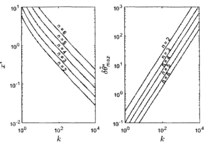
is then defined as the lower bound in (2.32) with a = I and a = 0.3, respectively, for the CRM and IC-adaptive systems. By setting A to the lower bound in (2.45), we show how x* and 6,*ax vary with
k in Figure 2-11 for the CRM-adaptive system and Figure 2-12 for the IC-adaptive system.
In these figures, results for system orders from two to six are shown.
It is clear from these graphs that the lower bound of t2 in (2.92) may be made arbitrarily
101 100 10'2 100~ 10 2 1 102/ 102 10~ 100 10 0 1 2 1 A-~ i0
Figure 2-11: x* and 0*x for versus k with n = 2 -÷ 6 in the CRM-adaptive system
101 S102 101 100 100 102 4 k 100 10'~ 100 102 104 k
Figure 2-12: x* and 8,* for versus k with n = 2 - 6 in the IC-adaptive system
for the CRM-adaptive system. Additionally, it can be seen that x* approaches a non-zero value as k increases for the IC-adaptive system, while x* approaches zero for the CRM-adaptive system. This means that )*O may be made arbitrarily small by increasing k for the CRM-adaptive system, but not for the IC-adaptive system.
2.4.2
Simulation Results
To illustrate sticking and the significance of Figures 2-11 and 2-12, simulations were car-ried out for a CRM and IC-adaptive system defined in Section 2.1.1 and 2.1.2, respectively,
by 0 1 0 0 A= 0 0 1 b= 0 (2.95) LO -4 -4 1 0 1 0 An, = 0 0 1 L= [03x31 (2.96) 1 -3 -3
with bn, = b for CRM-adaptive system and defined in (2.14) for the IC-adaptive system. For
the CRM-adaptive system, an adaptive controller as in (2.3) and (2.4) was simulated where P in (2.4) was solved using (2.8) with Qo = I. For the IC-adaptive system, an adaptive controller as in (2.15) and (2.16) was simulated with the same P. A constant reference input was chosen with r(t) = 1 and the system was initialized at t1 = 0 as
x(ti) = 0 Xm(ti) = 0 6(ti) =[O0,jol1O]. (2.97)
For each simulation, the initial conditions in (2.97) were used for increasingly negative values of O0 while recording the settling time T defined as
Tmin t 14 -1< E (2.98)
(t)~ |zti T|| l~_,
where z(t) = [x(t), xm(t), ®(t)]T, z* = limt z(t) and E = 0.05. By making 6O more negative in (2.97), the system was initialized further and further into a sticking region (This corresponds similarly to increasing k in (2.94)). The results of the settling time T are included in Figure 2-13. Here a decreasing convergence rate for the CRM-adaptive system is observed as O0 is made more negative. On the other hand, the IC-adaptive system demonstrates a constant learning rate. Figure 2-13 also includes the settling time T for the exponentially stable system (denoted by 'EXP-system') when 0(t) = 0 V t. Here x(ti)
#
0 such thatIIz(ti)I
# 0. This additional plot is only included to create a perspective of the convergence rate of the ORM and IC adaptive systems against a roughly equivalentexponentially stable system. ORM-system 10 20 30 40 40 35 30 25 20 15 10 5 0 IC-system 10 20 30 40
~Iz(ti)il
40 35 30 25 20 15 10 5 0 -EXP-system 10 20 30 40Figure 2-13: Settling time T for systems
various initial conditions of the CRM and IC-adaptive
2.4.3
Additional Insight to Sticking in the IC-Adaptive System
The results in Sections 2.3 and 2.4 thus far demonstrate that the IC-adaptive system is less susceptible to sticking when compared to the CRM-adaptive system. Consider again Section 2.1.2: An alternate comparison can be drawn between the two adaptive systems when we note that (2.15) may be written as
u(t) [02(t) ... On(t)]xp(t) + O1 (t)
]
[Cpxp(r) - r(T)]d (2.99) where 0(t) = [01 (t), 02(t) ... ,,(t)]. Let Op(t) = [02(t) ... 0, (t)] andrp(t) - q * 1 (t)
j
[Cpxp( ) - r( r)]d. (2.100)Then (2.99) takes the familiar form
it(t) = Op(t)xp(t )+q*rp(t). (2.101)
With this in mind, we compare the IC-adaptive plant differential equation (2.10) and con-troller (2.101), directly to (2.2) and (2.3) of the CRM-adaptive system. If the order of these
2000 1500 1000 H 500 0
two plants were the same and (A, b) in (2.2) was equal to (A,, bp) from (2.10), then we expect a very similar result could be drawn from Theorem 2 where the plant states were characterized. This would be the case, but r, (t) in (2.100) contains a time varying parame-ter Oi (t) and an integrated error state eyi(t) f [Cx,((r) - r(r)]dr. Unlike the reference
input r(t) in (2.3), r,(t) introduces an additional degree of freedom that reduces the effects of sticking. It can be seen form (2.29) through (2.32) that the definition of the sticking region Y/ is largely dependent on the reference input bounds r* and r,.
2.5
Sticking Analysis with (A,
Ab)
unknown
Thus far in this chapter, we have proved the existence of sticking region in the CRM and IC-adaptive systems for the case when only A in (2.2) and (2.13) was unknown. Consider now the nW order time-invariant plant differential equation is given by
x(t) = Ax(t)+ Xbu(t). (2.102)
In this section, we consider the CRM-adaptive system for the case when (A, Xb) is un-known. Here it is assumed that the vector b is known while A is an unknown constant with a known sign. Once again, only the single input case is considered and it is assumed that the underlying reference input is bounded and smooth. From the numerical analysis in Section 2.4.1, we show that the IC-adaptive system is less susceptible to sticking compared to the CRM-adaptive system. This result could be more intuitively understood from the additional insight provided in Section 2.4.3. Using the same intuitive approach, the effect due to the additional unknown parameter on sticking will be investigated.
In this section we first present the underlying adaptive system when (A, Xb) is un-known. The effect of the additional unknown parameter on sticking is then discussed. Finally, simulations are included to verify the result.
2.5.1
The CRM-Adaptive System with (A, Xb) Unknown
The n'h order time-invariant plant differential equation is given by
f(t) = Ax(t) + Abu(t)
where A is a constant n x n unknown matrix, b is a known vector of size it and unknown scalar with a known sign. A state variable feedback controller is defined
u(t) = OA X(t) +OB(t) r(t)
where OA(t) and OB(t) are time varying adaptive parameter updated as
®A(t) = -sign(X)b TPe(t)xT(t)
OB(t)
= -sign(A)bTPe(t)r(t)(2.103)
A is an
by
(2.104)
(2.105)
Here e(t) = x(t) - x,, (t) and xn (t) is the output of a reference model defined by
(2.106)
where A.. is Hurwitz and L is a constant n x n feedback matrix which introduces a closed-loop in the reference model. With the standard matching conditions [10]
A+ A be* = A
A bO* = bm
satisfied, the error differential equation is defined by
d(t) = [A, - L]e(t) + Xb6A (t)x(t) + XbeB(t)r(t)
(2.107)
(2.108)
where 6A(t) = OA(t) - 0* and 6B(t)
-t ~ - If An -L] is Hurwitz, then a
sym-metric positive definite P exists that solves the well known Lyapunov equation
[Am -L]PP + pAm -L]
=
-Q0 (2.109)where Qo is a symmetric positive definite matrix. It is well known that the error model in
(2.108) and (2.105) can be shown to be globally stable at the origin and that [10]
lim e(t) = 0. (2.110)
t-*oo
2.5.2
Insight to Sticking in the CRM-Adaptive System with (A, 2Lb)
Unknown
Using the same approach as presented in Section 2.4.3, we note that the controller in (2.104) may be expressed as
-(t)
= ®E(t)x(t) + q*rB(t) (2.111)
where
r-B(t) = q* OB(t)r(t).
(2.112)
With this in mind, we compare the CRM-adaptive plant and controller with (A, Xb) un-known in (2.103) and (2.104), directly to (2.2) and (2.3) of the CRM-adaptive system with only (A) unknown. If (A, Xb) in (2.103) was equal to (A, b) form (2.2), then we expect a very similar result could be drawn from Theorem 2 where the plant states were charac-terized. Once again, this would be the case but rB(t) in (2.112) contains a time varying parameter OB(t), which unlike the reference input r(t) in (2.3), introduces an additional
degree of freedom that reduces the effects of sticking.
This is a similar result to Section 2.4.3. In order to demonstrate these effects, simulation results are included in the following section.
2.5.3
Simulation Results
Rather than completing an entire sticking analysis for the CRM-adaptive system with
(A, Ab) unknown, we complete a convergence analysis as done in Section 2.4.2.
Sim-ulations were carried out for the CRM-adaptive system with (A) and (A, Ab) unknown as defined in Sections 2.1.1 and 2.5.1, respectively. The plant and reference models are defined by
0
1
0
A =K
0 1 0L -4 -- 4 0 1 0 All= 0 0 1 -1 -- 3 -30
b= 0b
ll
b~b (2.113) (2.114) L= [03x3]For the CRM-adaptive system with (A) unknown, an adaptive controller as in (2.3) and (2.4) was simulated where P in (2.4) was solved using (2.8) with Qo = I. For the CRM-adaptive system with (A, Ab) unknown, an CRM-adaptive controller as in (2.104) and (2.105) was simulated with the same P and A = 1. A constant reference input was chosen with
r(t) 1 and the system was initialized at t1 = 0 as
x(ti) = 0 x,.( ) = 0 6(t) = A(tl) = [60, 60,o] eB(t) =0. (2.115)
For each simulation, the initial conditions in (2.115) were used for increasingly negative values of Oo while recording the settling time T defined as in (2.98) where
CRM with only (A) unknown CRM with (A, Ab) unknown,
(2.116)
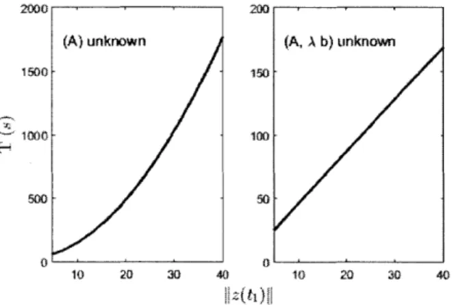
z* = lim ,z(t) and E = 0.05. By making 0 more negative in (2.97), the system was initialized further and further into a sticking region. The results of the settling time T are included in Figure 2-14. As before, a decreasing convergence rate for the CRM-adaptive
ZI(t) = [x(t), xin(t), 6(t)]T
system with only (A) unknown is observed as 0o is made more negative. On the other hand, the CRM-adaptive system with (A, AXb) unknown demonstrates a constant learning rate similarly to the IC-adaptive system in Figure 2-13. This corresponds to the discussion form Section 2.5.2.
200G 200
(A) unknown (A, A b) unknown
1500 150
1000-
100-500 50
10 20 30 40 10 0 3 4
Figure 2-14: Settling time T for various initial conditions of the CRM-adaptive systems with (A) and (A, Ab) unknown
2.6 Summary
In this chapter, we have focused on slow convergence properties of errors in a class of adaptive systems that corresponds to adaptive control of linear time-invariant plants with state variables accessible. We prove the existence of a sticking region in the error space where the state errors move with a finite velocity independent of their magnitude. These properties are exhibited by ORM, CRM and IC-adaptive systems. Simulation and numer-ical studies are included to illustrate the size of this sticking region and its dependence on various system parameters.
Chapter 3
Sticking in Outer-Loop Control
Chapter 2 presents an analytic approach for characterizing sticking regions in adaptive systems. In this chapter, the impact of sticking is investigated for outer-loop controllers that include inner-loop adaptation. An analysis is presented that identifies the existence of a sticking region in the inner-loop and its impact on command following in the outer-loop. In the design of outer-loop controllers, it is often assumed that the inner-loop states are readily available. The inner control loop is then responsible for tracking command signals generated by the outer-loop. This separates the outer and inner-loop design problems which is advantageous since well-established design methods exist separately [12]. However, if inner-loop adaptation is implemented to account for any uncertainties in the plant model, then it is possible, as argued in Chapter 2, that the overall inner-loop adaptive system can exhibit sticking, and as a result, the outer-loop performance in terms of command tracking can be compromised.
In order to demonstrate these sticking effects in outer-loop control, we focus on a com-bined inner and outer-loop problem in a flight control application. Here, adaptation is implemented in the inner-loop for control of an aircraft's angle of attack and pitch rate dynamics with uncertainties. This forms the inner-loop dynamics of the system. The outer-loop dynamics consists of the pitch angle and altitude of the aircraft, and is assumed to be known. Two adaptive control solutions are implemented that ensure the aircraft altitude tracks the desired altitude. While the controllers are very similar, they exhibit different behaviors during sticking. Through simulations it is shown that one of these controllers is
not able to access the inner-loop states necessary for effective altitude command tracking during sticking. Thus the importance of accounting for sticking regions in adaptive control is demonstrated.
3.1
Problem Statement
We consider the general outer-loop control problem when the inner-loop dynamics are un-known. Model reference adaptive control may be implemented to account for the uncertain-ties in the inner-loop. However, following this approach, the system becomes susceptible to inner-loop sticking as presented in Chapter 2. In this section, we present the under-lying outer-loop control problem when there are uncertainties in the inner-loop dynamics and propose a control design. With this, the overall problem with regard to the impact of inner-loop sticking on outer-loop control is stated.
3.1.1
The Outer-Loop Control Problem with Unknown Inner-Loop
Dynamics
Consider the ng order differential equation that describes the unknown inner-loop dynam-ics given by
p (t ) = A pxp (t )
+
bp t(t ) (3.1 )where Ap is a constant unknown n x i, matrix and bp is a known vector of size tip. Additionally we have the known outer-loop dynamics given by the nW order differential
g equation
g
t ) = Agxg(t)+
B9xpt W(3.2)
y(t ) =Cgxg(t ).
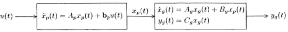
It is assumed that the open-loop plant, as shown in Figure 3-1, is controllable with acces-sible states xp(t) and xg(t). Let vg,(t) be a desired command state which is known and specified. The objective is to design a closed-loop controller u(t) such that the system is
'(t) 'XIA0 y (t) =Cqax,(t)
Figure 3-1: Open-loop plant with inner and outer-loop dynamics
stable and the outer-loop state y. (t) approaches the desired trajectory yct (t), that is
lim yg (t = yga,,d (t).- (3.3)
t-+0
In this chapter, the control problem is solved by first designing an open-loop reference model (ORM) where the unknown parameters of the system are estimated. Here the ORM is designed such that it represents the output desired in the plant at every time (i.e. achieves tracking of the trajectory yg,(t)). Since the dynamics of the reference model may vary from the actual plant, error states are defined. A control architecture similar to that in [14] is then implemented, where additional error state feedback loops are introduced to the ORM, thus forming a closed-loop reference model (CRM). By considering the error dynamics between the actual system and the CRM, an adaptive controller u(t) may be designed to achieve the control objective in (3.3).
The complete control design of u(t) will follow in Section 3.3. In order to present the main idea of this chapter, the following proposition is useful, which is
Proposition 7. If the uncertainties of the inner-loop dynamics in (3.1) are such that the matching conditions
Ap+ bpO* = A,,,,, and b = bp (3.4)
are satisfied for some 0*, where Arm and bpm are known, then there exists an adaptive controller of the form
-(t)
= op(t)xp(t)+ fp (t) (3.5)
where Op(t) and fp(t) are time varying functions with the properties Op(t), Op(t ), fp(t),
fp(t)
c
Y. such that the system response satisfies xp(t) xg (t) E Y. and the controlobjec-tive in (3.3) is realized.
model discussed in Chapter 2. We will return to the definition of (A,, bp,,) in Section
3.3.
3.1.2
Impact of Inner-Loop Sticking on Outer-Loop Control
Proposition 7 implies that an adaptive controller exists such that the control objective in
(3.3) is satisfied. However, by comparing the form of (3.5) to (2.3), we realize the
inner-loop may be susceptible to sticking. Thus we begin our approach by completing a stick-ing analysis as done in Theorem 2 under Proposition 7: Show that there are some initial conditions for which .~p(t) will remain in a set N while Op(t) traverses in a set S over a certain time interval [tl, t2]. From (3.2), we see that if xp(t) is subject to the constraint kp(t) E N Vt E [ti, t2] during sticking, then the ability for yg(t) to converge quickly towards Ygcilld (t) may be prohibited during this time interval.
This is problematic since we have shown in Chapter 2 that sticking may occur for extended periods of time. In this chapter, we are only concerned about the definition of sets
S and N. Therefore, in this chapter "sticking" will refer to the time interval [ti, t2] during
which 6(t) E S and k(t) E N.
3.2
Analyis of Sticking in Outer-Loop Control
In this section, we complete a sticking analysis as done in Theorems 2 and 6 for the inner-loop of the system as given in (3.1). This is completed using the control solution from Proposition 7 (to be proved in Section 3.3 which addresses the design of an autopilot system for altitude tracking). With this sticking analysis, the impact on outer-loop control will be investigated.
3.2.1
Inner-Loop Sticking
Suppose that the matching condition is satisfied for a suitably chosen (Ap, bp,) and that a control input as in (3.5) exists. We can then express the plant differential equation in (3.1)


![Figure 3-2: Longitudinal flight angle relations [9]](https://thumb-eu.123doks.com/thumbv2/123doknet/14174840.475128/53.918.232.656.286.490/figure-longitudinal-flight-angle-relations.webp)
