Bitwise: optimizing bitwidths using data-range propagation

Bitwise: Optimizing Bitwidths Using Data-Range

Propagation

by

Mark William Stephenson

Submitted to the Department of Electrical Engineering and Computer

Science

in partial fulfillment of the requirements for the degree of

Master of Science in Computer Science and Engineering

at the

MASSACHUSETTS INSTITUTE OF TECHNOLOGY

May 2000

@

Mark William Stephenson, MM. All rights reserved.

The author hereby grants to MIT permission to reproduce and

distribute publicly paper and electronic copies of this thesis document

in whole or in part.

ENG

A uthor ...

JUN 2 2

2000

Department of Ele

ical Engineering and Computer Science

/7

_{May 5, 2000}

Certified by..

2

Saman Amarasighe

Assistant Professor

Thesis Supervisor

Accepted by ... (

Arthur C. Smith

Chairman, Department Committee on Graduate Students

Bitwise: Optimizing Bitwidths Using Data-Range

Propagation

by

Mark William Stephenson

Submitted to the Department of Electrical Engineering and Computer Science on May 5, 2000, in partial fulfillment of the

requirements for the degree of

Master of Science in Computer Science and Engineering

Abstract

This thesis introduces Bitwise, a compiler that minimizes the bitwidth - the number of bits used to represent each operand - for both integers and pointers in a pro-gram. By propagating static information both forward and backward in the program dataflow graph, Bitwise frees the programmer from declaring bitwidth invariants in cases where the compiler can determine bitwidths automatically. Because loop in-structions comprise the bulk of dynamically executed inin-structions, Bitwise incorpo-rates sophisticated loop analysis techniques for identifying bitwidths. We find a rich opportunity for bitwidth reduction in modern multimedia and streaming application workloads. For new architectures that support sub-word data-types, we expect that our bitwidth reductions will save power and increase processor performance.

This thesis also applies our analysis to silicon compilation, the translation of programs into custom hardware, to realize the full benefits of bitwidth reduction. We describe our integration of Bitwise with the DeepC Silicon Compiler. By taking advantage of bitwidth information during architectural synthesis, we reduce silicon

real estate by 15 - 86%, improve clock speed by 3 - 249%, and reduce power by 46

-73%. The next era of general purpose and reconfigurable architectures should strive

to capture a portion of these gains.

Thesis Supervisor: Saman Amarasighe Title: Assistant Professor

Acknowledgments

First and foremost I'd like to thank my advisor Saman Amarasinghe for sinking a great deal of time and energy into this thesis. It was great working with him. Jonathan Babb also helped me a great deal on this thesis. I'd like to thank him for letting me use his silicon compiler to test the efficacy of my analysis.

I also received generous help from the Computer Architecture Group at MIT. In

particular, I want to thank Matt Frank, Michael Zhang, Sam Larsen, Derek Bruening, Andras Moritz, Benjamin Greenwald, Michael Taylor, Walter Lee, and Rajev Barua for helping me in various ways. Special thanks to Radu Rugina for providing me with his pointer analysis package. Thanks to the National Science Foundation for funding me for the last two years.

This research was funded in part by the NSF grant EIA9810173 and DARPA grant DBT63-96-C-0036.

Contents

1 Introduction 11

1.1 A New Era: Software-Exposed Bits . . . . 11

1.2 Benefits of Automating Bitwidth Specification . . . . 12

1.3 The Bitwise Compiler . . . . 13

1.4 Application to Silicon Compilation . . . . 13

1.5 Contributions . . . . 14

1.6 O rganization . . . . 14

2 Bitwidth Analysis 15 3 Bitwise Implementation 17 3.1 Candidate Lattices . . . . 17

3.1.1 Propagating the Bitwidth of Each Variable . . . . 17

3.1.2 Maintaining a Bit Vector for Each Variable . . . . 18

3.1.3 Propagating Data-Ranges . . . . 18 3.2 Data-Range Propagation . . . . 19 4 Loop Analysis 25 4.1 Closed-Form Solutions . . . . 25 4.2 Sequence Identification . . . . 26 4.3 Sequence Example . . . . 28 4.4 Term ination . . . . 31

5 Arrays, Pointers, Globals, and Reference Parameters

5.1 A rrays . . . .

5.2 P ointers . . . .

5.3 Global Variables and Reference Parameters . . . .

6 Bitwise Results

6.1 Experiments . . . .

6.2 Register Bit Elimination . . . .

6.3 Memory Bit Elimination . . . . 6.4 Bitwidth Distribution . . . .

7 Quantifying Bitwise's Performance 7.1 DeepC Silicon Compiler . . . .

7.1.1 Implementation Details . . . . .

7.1.2 Verilog Bitwidth Rule . . . . .

7.2 Impact on Silicon Compilation . . . . .

7.2.1 Experiments . . . .

7.2.2 Registers Saved in Final Silicon

7.2.3 A rea . . . . 7.2.4 Clock Speed . . . . 7.2.5 Power . . . . 7.2.6 Discussion . . . . 8 Related Work 9 Conclusion 33 33 34 35 37 . . . . 37 . . . . 39 . . . . 40 . . . . 41 47 47 48 48 48 49 49 51 53 53 . . . . . 55 57 59

List of Figures

2-1 Sample C code to illustrate fundamentals. . . . .

3-1 Three alternative data structures for bitwidth analysis. . . . . 3-2 Forward and backward data-range propagation. . . . .

3-3 A selected subset of transfer functions for data-range propagation.

4-1 Pseudocode for the algorithm that solves closed-form solutions. . . 4-2 A lattice that orders sequences according to set containment. . . . . . 4-3 Exam ple loop. . . . . 4-4 SSA graph corresponding to example loop .. . . . . 4-5 A dependence graph of sequences... 4-6 Backward propagation within loops. . . . .

6-1 Com piler flow . . . .

6-2 Percentage of total register bits. . . . .

6-3 Percentage of total memory remaining after bitwidth analysis. . . 6-4 A bitspectrum of the benchmarks we considered. . . . .

7-1 7-2 7-3

7-4

7-5

Register bits after Bitwise optimization. . . . .

Register bit reduction in final silicon. . . . .

FPGA area after Bitwise optimization. . . . . FPGA clock speed after Bitwise optimization. . . . . ASIC power after Bitwise optimization. . . . .

16 18 21 23 27 28 29 29 30 32 38 41 43 44 . . . 50 . . . 50 . . . 52 . . . 54 . . . 55

List of Tables

6.1 Benchmark characteristics . . . . 39 6.2 Number of bits in programs before and after bitwidth analysis . . . . 42

6.3 Table showing memory bits remaining after bitwidth analysis. .... 43 6.4 The bitspectrum in tabular format. . . . . 45

Chapter 1

Introduction

The pioneers of the computing revolution described in Steven Levy's book

Hack-ers [16] competed to make the best use of every precious architectural resource. They

hand-tuned each program statement and operand. In contrast, today's programmers pay little attention to small details such as the bitwidth (e.g., 8, 16, 32) of data-types used in their programs. For instance, in the C programming language, it is common to use a 32-bit integer data-type to represent a single Boolean variable. We could dismiss this shift in emphasis as a consequence of abundant computing resources and expensive programmer time. However, there is another historical reason: as processor architectures have evolved, the use of smaller operands eventually has provided no performance gains. Datapaths became wider, but the processor's entire data path was exercised regardless of operand size. In fact, the additional overhead of pack-ing and unpackpack-ing words - now only to save space in memory - actually reduces performance.

1.1

A New Era: Software-Exposed Bits

Three new compilation targets for high-level languages are re-invigorating the need to conserve bits. Each of these architectures expose subword control. The first is the rejuvenation of SIMD architectures for multimedia workloads. These architectures include Intel's MultiMedia eXtension (MMX) and Motorola's Altivec [19, 24]. For

example, in Altivec, data paths are used to operate on 8, 16, 32, or 64 bit quantities. The second class of compilation targets consists of embedded systems which can effectively turn off bit slices [6]. The static information determined at compile time can be used to specify which portions of a datapath are on or off during program execution. Alternatively, for more traditional architectures this same information can be used to predict power consumption by determining which datapath bits will change over time.

The third class of compilation targets comprises fine-grain substrates such as gate and function-level reconfigurable architectures - including Field Programmable Gate Arrays (FPGAs) - and custom hardware, such as standard cell ASIC designs. In both cases, architectural synthesis is required to support high-level languages. There has been a recent surge of both industrial and academic interest in developing new reconfigurable architectures [17].

Unfortunately, there are no available commercial compilers that can effectively target any of these new architectures. Programmers have been forced to revert to writing low-level code. MMX libraries are written in assembly in order to expose the most sub-word parallelism. In the Verilog and VHDL hardware description languages, the burden of bitwidth specification lies on the programmer. To compete in the marketplace, designers must choose the minimum operand bitwidth for smaller, faster, and more energy-efficient circuits.

1.2

Benefits of Automating Bitwidth Specification

Automatic bitwidth analysis relieves the programmer of the burden of identifying and specifying derivable bitwidth information. The programmer can work at a higher level of abstraction. In contrast, explicitly choosing the smallest data size for each operand is not only tedious, but also error prone. These programs are less malleable since a simple change may require hand propagation of bitwidth information across a large segment of the program. Furthermore, some of the bitwidth information may be dependent on a particular architecture or implementation technology, making

programs less portable.

Even if the programmer explicitly specifies operand sizes in languages that allow it, bitwidth analysis can still be valuable. For example, bitwidth analysis can be used to verify that specified operand sizes do not violate program invariants - e.g., array

bounds.

1.3

The Bitwise Compiler

Bitwise minimizes the bitwidth required for each static operation and each static assignment of the program. The scope of Bitwise includes fixed-point arithmetic, bit manipulation, and Boolean operations. It uses additional sources of information such as type casts, array bounds, and loop iteration counts to refine variable bitwidths. We have implemented Bitwise within the SUIF compiler infrastructure [25].

In many cases, Bitwise is able to analyze the bitwidth information as accurately as the bitwidth information gathered from run-time profiles. On average we reduce the size of program scalars by 12 - 80% and program arrays by up to 93%.

1.4

Application to Silicon Compilation

In this thesis we apply bitwidth analysis to the task of silicon compilation. In partic-ular, we have integrated Bitwise with the DeepC Silicon Compiler [2]. The compiler produces gate-level netlists from input programs written in C and FORTRAN. We compare end-to-end performance results for this system both with and without our bitwidth optimizations. The results demonstrate that the analysis techniques per-form well in a real system. Our experiments show that Bitwise favorably impacts area, speed, and power of the resulting circuits.

1.5

Contributions

This thesis' contributions are summarized as follows:

" We formulate bitwidth analysis as a value range propagation problem.

* We introduce a suite of bitwidth extraction techniques that seamlessly perform bi-directional propagation.

" We formulate an algorithm to accurately find bitwidth information in the

pres-ence of loops by calculating closed-form solutions.

" We implement the compiler and demonstrate that the compile-time analysis can

approach the accuracy of run-time profiling.

" We incorporate the analysis in a silicon compiler and demonstrate that bitwidth

analysis impacts area, speed, and power consumption of a synthesized circuit.

1.6

Organization

The rest of the thesis is organized as follows. Chapter 2 defines the bitwidth analysis problem. Bitwise's implementation and our algorithms are described in Chapters 3, 4, and 5. Chapter 6 provides empirical evidence of the success of Bitwise. Next, Chap-ter 7 describes the DeepC Silicon Compiler and the impact that bitwidth analysis has on silicon compilation. Finally, we present related work in Chapter 8 and conclude in Chapter 9.

Chapter 2

Bitwidth Analysis

The goal of bitwidth analysis is to analyze each static instruction in a program to determine the narrowest return type that still retains program correctness. This information can in turn be used to find the minimum number of bits needed to represent each program operand.

Library calls, I/O routines, and loops make static bitwidth analysis challenging. In the presence of these constructs, we may have to make conservative assumptions about an operand's bitwidth. Nevertheless, with careful static analysis, it is possible to infer bitwidth information.

Structures such as arrays and conditional statements provide us with valuable bitwidth information. For instance, we can use the bounds of an array to set an index variable's maximum bitwidth. Other program constructs such as AND-masks, divides, right shifts, type promotions, and Boolean operations are also invaluable for reducing bitwidths.

The C code fragment in Figure 2-1 exhibits several such constructs. This code, which is an excerpt of the adpcm benchmark presented later in this thesis, is typical of important multimedia applications. Each line of code in the figure is annotated with a line number to facilitate the following discussion.

Assume that we do not know the precise value of delta, referenced in lines (1),

(1) index += indexTable[delta]; (2) if ( index < 0 ) index = 0; (3) if ( index > 88 ) index = 88; (4) step = stepsizeTable[index]; (5) (6) if ( bufferstep ) {

(7) outputbuffer = (delta << 4) & Oxf0;

(8) } else {

(9) *outp++ = (delta & OxOf) I

(10) (outputbuffer & Oxf0);

(11) }

(12) bufferstep = !bufferstep;

Figure 2-1: Sample C code used to illustrate the fundamentals of the analysis. This code fragment was taken from the loop of adpcm-coder in the adpcm multimedia benchmark.

value is confined by the base and bounds of indexTable'. Though we still do not

know delta's precise value, by restricting the range of values that it can assume, we effectively reduce the number of bits needed to represent it. In a similar fashion, the code on lines (2) and (3) ensure that index's value is restricted to be between 0 and

88.

The AND-mask on line (7) ensures that outputbuffer's value is no greater than Oxf 0. Similarly, we can infer that the assignment to *outp on line (9) is no greater than Oxff (0x0f I Oxf 0).

Finally, we know that bufferstep's value is either true or false after the

assign-ment on line (12) because it is the result of the Boolean not (!) operation.

'Our analysis assumes that the program being analyzed is error free. If the program exhibits bound violations, arithmetic underflow, or arithmetic overflow, changing operand bitwidths may alter its functionality.

Chapter 3

Bitwise Implementation

The next three chapters describe the infrastructure and algorithms of Bitwise, a compiler that performs bitwidth analysis. Bitwise uses SSA as its intermediate form. It performs a numerical data flow analysis. Because we are solving for absolute numerical bitwidths, the more complex symbolic analysis is not needed [22].

We continue by comparing the candidate data-flow lattices that were considered in our implementation.

3.1

Candidate Lattices

We considered three candidate data-structures for propagating the numerical infor-mation of our analysis. Figure 3-1 visually depicts the lattice that corresponds to each data-structure.

3.1.1

Propagating the Bitwidth of Each Variable

Figure 3-1 (a) is the most straightforward structure. While this representation permits an easy implementation, it does not yield accurate results on arithmetic operations. When applying the lattice's transfer function, incrementing an 8-bit number always produces a 9-bit resultant, even though it may likely need only 8-bits. In addition, only the most significant bits of a variable are candidates for bit-elimination.

INT,,n = min(IN7) TDR = (INTmin, INT.)

BW 32 INTx = nmax(INT)

I ~~(INTmin, INTax -1) (INTm.in.+ 1,INT,_)

31 TBL TBL TBL

(INTmin INTma -2) (INTi, + 1, INTax- I) (INTn, + 2, INT,)

1 0 10 10 1,

0 J-BL -LBL -BL (INTmin, INT,j) (INT, + 1, INTwjin+ 1) ... (-1, -1)(O0 0) (1, 1) ... (INT,, - 1, INTax-1)(INT., INT..

IBW

'DR

(a) (b) (c)

Figure 3-1: Three alternative data structures for bitwidth analysis. The lattice in (a) represents the number of bits needed to represent a variable. The lattice in (b) represents a vector of bits that can be assigned to a variable, and the lattice in (c) represents the range of values that can be assigned to a variable.

3.1.2

Maintaining a Bit Vector for Each Variable

Figure 3-1(b) is a more complex representation, requiring the composition of several

smaller bit-lattices [7, 20]. Although this lattice allows elimination of arbitrary bits

from a variable's representation, it does not support precise arithmetic analysis. As an example of eliminating arbitrary bits, consider a particular variable that is assigned the values from the set {0102, 1002, 11021. After analysis, the variable's bit-vector will

be [TT], indicating that we can eliminate the least significant bit. Like the first data

structure, the arithmetic is imprecise because the analysis must still conservatively assume that every addition results in a carry.

3.1.3

Propagating Data-Ranges

Figure 3-1(c) is the final lattice we considered. This lattice is also the implementation chosen in the compiler. A data-range is a single connected subrange of the integers from a lower bound to an upper bound (e.g., [1..100] or [-50..50]). Thus a data-range keeps track of a variable's lower and upper bounds. Because only a single range is

used to represent all possible values for a variable, this representation does not permit the elimination of low-order bits. However, it does allow us to operate on arithmetic

expressions precisely. Technically, this representation maps bitwidth analysis to the

to be useful in value prediction, branch prediction, constant propagation, procedure cloning, and program verification [18, 22].

For the Bitwise compiler we chose to propagate data-ranges, not only because of their generality, but also because most important applications use arithmetic and will benefit from their exact precision. Unlike a regular set union, we define the data-range union operation (Li) to be the union over the single connected subrange of the integers where (a,, ah) H (bl, bh) - (min(a,, bl), max(ah, bh)). We also define the data-range intersection operation (n1) to be the set of all integers in both subranges where

(a,, ah) n (bi, bh) = (max(a,, bi), min(ah, bh)). The intersection of two non-overlapping

data-ranges yields the value J-DR, which can be used to identify likely programmer errors (e.g., array bound violations). Additionally, note that the value TDR, a part

of the lattice, represents values that cannot be statically determined, or values that can potentially utilize the entire range of the integer type.

3.2

Data-Range Propagation

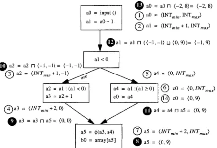
As concluded in the last section, our Bitwise implementation propagates data-ranges. These data-ranges can be propagated both forward and backward over a program's control flow graph. Figure 3-3 shows a subset of the transfer functions for propagation. The forward propagated values in the figure are subscripted with a down arrow ( ), and the backward propagated values with an up arrow (t). In general the transfer functions take one or two data-ranges as input and return a single data-range.

Initially, all of the variables in the SSA graph are initialized to the maximum range allowable for their type. Informally, forward propagation traverses the SSA graph in breadth-first order, applying the transfer functions for forward propagation. Because there is one unique assignment for each variable in SSA form, we can restrict a variable's range if the result of its assignment is less than the maximum data-range of its type.

To more accurately gather data-ranges, we extend standard SSA form to include the notion of range-refinement functions. For each node that is control dependent, a

function is created which refines the range of control variables based on the outcome of the branch test. Consider the SSA graph shown in Figure 3-2. Range-refinement functions have been inserted in each of the nodes directly following the branch test.

By taking control-dependent information into account, these functions facilitate a

more accurate collection of data-ranges. Thus, if the branch in the figure is taken, we know that al's value is less than zero. Similarly, al's value has to be greater than or equal to zero if the branch is not taken.

Forward propagation allows us to identify a significant number of unused bits, sometimes achieving near optimal results. However, additional minimization can be achieved by integrating backward propagation. For example, when we find a data-range that has stepped outside of known array bounds, we can back-propagate this new reduced data-range to instructions that have already used its deprecated value to compute their results. Beginning at the node where the boundary violation is found, we propagate the reduced data-range in a reverse breadth-first order, using the transfer functions for backward propagation. This halts when either the graph's entry node is reached, or when a fixed point is reached. Forward propagation resumes from this point.

Forward and backward propagation steps have been annotated on the graph in Figure 3-2 to ease the following discussion. The numbers on the figure chronologi-cally order each step. The step numbers in black represent the backward propagation of data-ranges. Without backward propagation we arrive at the following data-ranges:

'SSA form is not an efficient form for performing backward propagation[11]. Bitwise currently

reverts to standard data-flow analysis techniques only when analyzing in the reverse direction. If efficiency in the less common case of backward propagation is a concern, our form of SSA could readily be converted to SSI form, which was designed for bi-directional data-flow analyses[l].

a aO = a r- (-2, 8)= (-2, 8)

aO = input () _{aO = (INT,,,, INTmajx)}

al = aO+1 _®a=

(INT,,, + 1, INTax) (al = al n ((-1, -1) u (0, 9))= (-1, 9) al <0

O

tiIN a2 = (INTin + 1,-i) a4 = (0, INTmax)

a2 = al: (al<0) a4 = al :(al 0) cO = (0, INTax)

a3 = a2+ 1 cO = a4 I cO = (0, 9)

a3 = (INT n,,,,+2,0) a4 = a4 n a5 = (0, 9) * a3 = a3 n a5 = (0, 0)

a5 = (a3, a4) a5 = (INTi,,l, +2, INTmax)

bO = array[a5]

*

Figure 3-2: Forward and backward data-range propagation. The numbers denote the order of evaluation. Application of forward propagation rules are shown in white, while backward propagation rules are shown in black. We use array's bounds information to tighten the ranges of some of the variables.

aO = (INTmin, INTmax) al = (INTmin + 1, INTmax) a2 = (INTmin + 1, -1) a3 = (INTmin + 2,0) a4 = (0, INTmax) a5 = (INTmin + 2, INTmax) cO (0, INTmax)

Let us assume we know that the length of the array, array, is 10 from its decla-ration. We can now substantially reduce the data-ranges of the variables in the graph with backward propagation. We use array's bound information to clamp a3's data-range to (0, 9). We then propagate this value backward in reverse breadth-first order

using the transfer functions for backward propagation. In our example, propagating

aO (-2, 8) al = (-1, 9) a2 = (-1, -1) a3 = (0,0) a4 = (0,9) a5 = (0, 9) cO = (0,9)

Reverse propagation can halt after ao's range is determined (step 13). Because cO uses the results of a variable that has changed, we have to traverse the graph in the forward direction again. After we confine cO's data-range to (0, 9) we will have reached a fixed point and the analysis will be complete.

In this example we see that data-range propagation subsumes constant propaga-tion; we can replace all occurrences of a3 with the constant value 0.

(a) bj = (bl, bh) C = _{(cl, ch)} at = (al, ah) a=b+c bT = bf l (al - ch, ah - c) Ct = cr i (al - bh, ah - bi) a, = at n (bi + cl, bh + Ch) (b) bj = (b, bh) _{c = (cI, ch)} bt = b nF (al + cz, ah + Ch) ct = c n (al + b, ah + bh) a = b-c

at = (al, ah) at = at n (bi - ch, bh - c)

(c) b = (bl, bh) bt = bg

cg = (c1, ch) _{ct = c}

a=b&c

aT =(alah)ag = aT n (-2n-1, 2n-1 - 1),

at =(l, ah) where n = min(bitwidth(bg), bitwidth(cg,))

(d) b = (bl,bh) b bbr-a

a b

a = (al, ah) a - a -1 b

(e) x = (al, ah) x = x F (x1, xh)

{XI <_ X < Xh}

xb = (bi, bh) xbT Xbj 1

xcI = (cch) Xb Xc Xct = X% Xa

xa .TbXc)

Xat = (al, ah) xa L at n (xb U X%)c

(g) Xa I = (al, ah) yJ = (y, yh) xbt = (bl,bh) xC T = (Ch, Ch) ba <y xb Xa. = X% F1 (xbT U X'T) XC b Xa n Xb (al,yh ₁₎ xc = Xa l Xc T n (yi, ah)

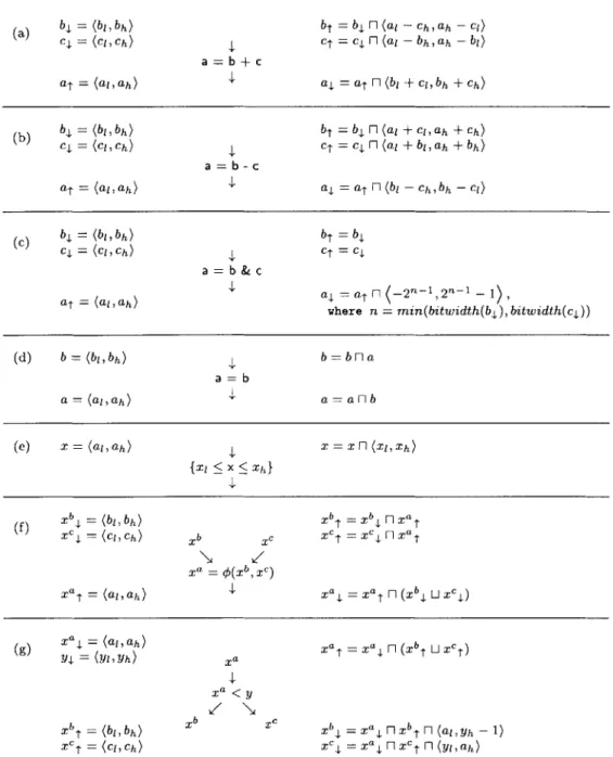
Figure 3-3: A selected subset of transfer functions for bi-directional data-range propagation. Intermediate results

on the left are inputs to the transfer functions on the right. The variables in the figure are subscripted with the direction in which they are computed. The transfer function in (a) adds two data-ranges, and (b) subtracts two data-ranges. Both of these functions assume saturating semantics which will confine the resulting range to be within the bounds of the type on which they operate. The AND-masking operation for signed data-types in (c) returns a data-range corresponding to the smallest of its two inputs. It makes use of the bitwidth function which returns the number of bits needed to represent the data-range. The type-casting operation shown in (d) confines the resulting range to be within the range of the smaller data-type. Because variables are initialized to the largest range that can be represented by their types, ranges are propagated seamlessly, even in the case of type conversion. The function in (e) is applied when we know that a value must be within a specified range. For instance, this rule is applied to limit the data-range of a variable that is indexing into a static array. Note that rules (d) and (e) are not directionally dependent. Rule (f) is applied at merge points, and rule (g) is applied at locations where control-flow splits. In rule

(g), we see that xb corresponds to an occurrence of xa such that xa < y. We can use this information to refine the

Chapter 4

Loop Analysis

Optimization of loop instructions is crucial - they usually comprise the bulk of

dynamic instructions. Traditional data flow analysis techniques iterate over back edges in the graph until a fixed point is reached. However, this technique will saturate even the simplest loop-carried arithmetic expression. That is, because the method does not take into account any static knowledge of loop bounds, such an expression will eventually saturate at the maximum range of its type.

Because many important applications use loop-carried arithmetic expressions, a new approach is required. To this end, our implementation of the Bitwise compiler identifies loops and finds closed-form solutions. We ease loop identification in SSA form by converting all q-functions that occur in loop headers to P-functions [9]. These functions have exactly two operands; the first operand is defined outside the loop, and the second operand is loop carried. We take advantage of these properties when finding closed-form solutions.

4.1

Closed-Form Solutions

To find the closed-form solution to loop-carried expressions, we use the techniques introduced by Gerlek et al. [9]. These techniques allow us to identify and classify

sequences in loops. A sequence is a mutually dependent group of instructions. In

dependence graph. We can examine the instructions of the sequence to try and find a closed-form solution to the sequence.

Thus, the algorithm begins by finding all the sequences in the loop. We then order them according to dependences between the sequences. At this point we can classify each sequence in turn. The algorithm for classifying sequences is shown in Figure 4-1.

A sequence's type is identified by examining its composition of instructions. This

functionality corresponds to the SEQUENCETYPE procedure called in Figure 4-1. We provide a sketch of our approach in Section 4.2.

Once we have determined the type of sequence the component represents, the algorithm invokes a solver to compute the sequence's closed-form solution. For each type of sequence, a different method is needed to compute the closed-form solution.

If no sequence is identified, the algorithm resorts to fixed point iteration up to a user

defined maximum.

4.2

Sequence Identification

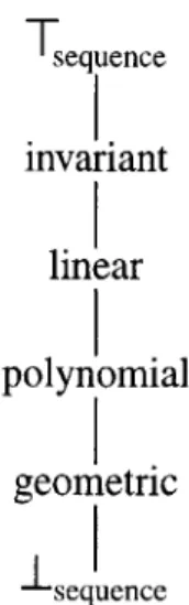
We sketch our sequence identification algorithm as follows. First, we create a partial order on the types of expressions we wish to identify. We employ the Expression lattice (Figure 4-2) to order various expressions according to set containment. For example, linear sequences are the composition of an induction variable and loop invariants, and polynomial sequences are the composition of loop invariants and linear sequences. The top of the lattice (Tsequence) represents an undetermined expression, and the bottom of the lattice (Isequence) represents all possible expressions.

Next, we create transfer functions for each instruction type in the source language.

A transfer function, which operates on the lattice, is implemented as a table that is

indexed by the expression types of its source operands. The destination operand is then tagged with the expression type dictated by the transfer function.

We proceed by classifying the sequence based on the types of its expressions and its composition of

#-

LSS: InstList List x Int Cur x Range Trip

x SSAVar Sentinel -+ Range x Int Range R +- (0,0)

Int i *- Cur

while i < IListj do

if List[i] has form (ak = p(al, am) with tripcount tc) then

ak -- al

(R, i) +- LSS(List,i + 1, tc xDR Trip, am) else if List[i] has form (ak = al linop C) then

ak <- a, linop C X DR Trip

else if List[i] has form (ak = #(al, am)) then

ak +- ai L am

if ak = Sentinel then return (ak,i)

i +- i + 1

return (R,i)

CLASSIFYSEQUENCE: InstList List -+ Void

Range Val

if jListj = 1 then

EVALUATEINST(List[0])

else

SeqType <- SEQUENCETYPE(List)

if SeqType = Linear then

(Val, x) +- LSS(List, 0, (1, 1) , NIL)

foreach Inst I E List do

ak <- Val where ak is destination of I

else if ...

else if SeqType = '-Sequence

Fix(List, MaxIters)

Figure 4-1: Pseudocode for the algorithm that classifies and solves closed-form solutions of commonly occurring sequences. The SEQUENCETYPE function identifies the type of sequence we are considering. Based on the sequence type, we can invoke the appropri-ate solver. We provide pseudocode for the linear sequence solver LSS. The Fix function

T

Figure 4-2: A lattice that orders sequences according to set containment.

linear sequences must have at least one p-function'. Remember that p-functions define loop headers, and thus denote the start of all non-trivial sequences. Trivial sequences contain exactly one instruction, and thus, the sequence itself represents the closed-form solution.

4.3

Sequence Example

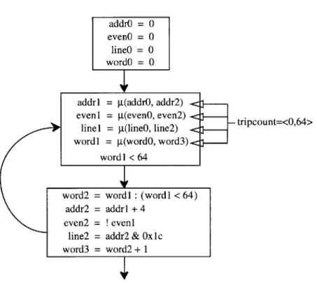
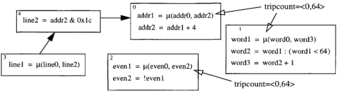
Figure 4-3 is an example loop and Figure 4-4 is its corresponding SSA graph. In this example all p-functions are annotated with the loop's tripcount ((0, 64)). While we can restrict the range of the loop's induction variable without the annotations, knowing the tripcount allows us to analyze other unrelated sequences.

The next step is to find all of the strongly connected components in the loop's body and create the sequence dependence graph. The sequence dependence graph for the loop in Figure 4-3 is shown in Figure 4-5.

We then analyze each of the sequences according to the dependence graph. The algorithm classifies the sequence based on the types of its constituent expressions. The component below, from the example, is determined to be a linear sequence be-cause it contains a [t-function and a linear-type expression:

1_{Gerlek et al. process inner-loops first and provide mechanisms to propagate closed-form solutions}

addr = 0; even = 0; line = 0; for (word addr = even = line = } = 0; word < 64; word++) addr + 4; !even;

addr & Ox1c;

Figure 4-3: Example loop.

addrO = 0

evenO = 0

line0 = 0 wordO = 0

addrl = g(addrO, addr2) even1 = g(evenO, even2)

line1 = g(lineO, line2)

wordi = g(word, word3). wordI < 64

- tripcount=<0,64>

Figure 4-4: SSA graph corresponding to example loop. {

word2 = wordi : (wordi < 64) addr2 = addrl + 4

even2 = ! eveni

line2 = addr2 & OxIc

word3 = word2 + 1

4 line2 = addr2 & OxIc addrl = p(addr, addr2)

tripcount=<0,64>

addr2 = addrl + 4

wordi = t(wordO, word3) word2 = wordI : (wordl < 64) linel = p(lineO, line2) even 1 = g(evenO, even2) word3 = word2 + 1

even2 = !evenl

tripcount=<O,64>

Figure 4-5: A dependence graph of sequences corresponding to the code in Figure 4-3. The sequences labeled (3) and (4) are trivial sequences. In other words, the sequences are themselves the closed-form solution. Using the tripcount of the loop, we can calculate the final ranges for the linear sequences labeled (0) and (1). Though we do not identify Boolean sequences such as the one marked (2), they quickly reach a fixed point.

Sequence Sum

addrl = p(addrO, addr2) (0,0)

addr2 = addrl + 4 (4, 4) x (0, 64) = (0, 256)

Based on the tripcount of the p-function ((0, 64)) and addr0's range ((0, 0)), the

function LSS in Figure 4-1 finds the maximum range that any of the variables in the linear sequence can possibly assume. The function steps through the sequence summing up all of the invariants. This sum is multiplied by the total number of times the loop in question will be executed. For this example, the function determines the

maximum range to be (0, 256). At this point we set all of the destination variables in

the sequence to this range and the sequence is solved. Note that this solution makes no distinction between the values of individual variables in the sequence.

Obtaining this conservative result is simpler than finding the precise range for each variable in the sequence. Because there is typically little variation between ranges of destination variables in the same sequence, this method works well in practice.

Unlike linear sequences, not all sequences are readily identifiable. In such cases

we iterate over the sequence until a fixed point is reached. For example, the sequence

labeled (2) in Figure 4-5, will reach a fixed point after only two iterations. Not

divides - all common in multimedia kernels - can quickly reach a fixed-point. The following section addresses the cases when a fixed-point is not reached quickly.

4.4

Termination

For cases in which we cannot find a closed-form solution, lattice height could lead to seemingly boundless iteration. For example, by traversing back-edges in the control flow graph, it could take nearly 232 iterations to reach a fixed point for typical 32-bit integers.

In order to solve this problem, we consider what happens to a data-range after applying a transfer function to a static assignment. The data-range either:

" reaches a fixed point, or " monotonically decreases.

Thus it is possible to add a user-defined limit to the number of iterations. When iteration is limited, the resulting data-range will be an improved but potentially sub-optimal solution.

4.5

Loops and Backward Propagation

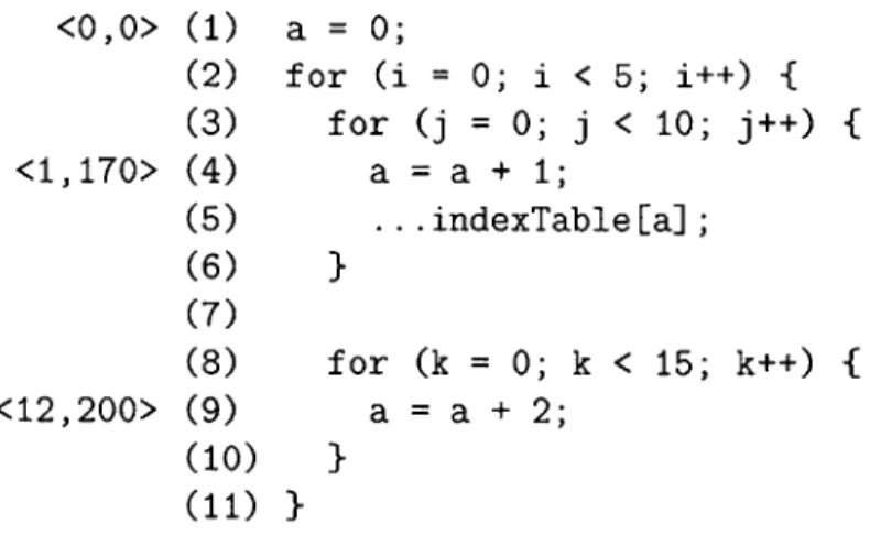
Because arrays are usually accessed within loop bodies (and are the principal form of known bounds information), backward propagation within loops is essential. It turns out that the DAG of sequences that was constructed for analyzing sequences in order, provides an excellent infrastructure for backward propagation within loops. For instance, if we find that an index variable steps beyond the range of an array in one of the loop's sequences, we can restrict the range, then backward propagate the new range using the dependence information inherent in the DAG.

Note that we cannot always use backward propagation within loops. For example, in the case of linear sequences, we do not precisely solve for the values of individual variables in the sequence. Because the value of a linear induction variable may in

<0,0> (1) a = 0; (2) for (i = 0; i < 5; i++){ (3) for (j = 0;

j

j++)

Figure 4-6: Sample C code used to illustrate the problems associated with backward prop-agation within loops. The actual data-range associated with each expression in the linear sequence is shown on the left of the figure. Our conservative solution will assign every expression in the sequence to the value (0, 200).

fact be different in two loop nests, our conservative approximation prevents us from restricting the entire sequence based on one variable.

Consider the example in Figure 4-6. Though the actual range of values that the expressions on line (4) and (9) can take on are different, we conservatively set them both to (0, 200). Because of this simplification however, we cannot use the bounds information on line (5) to restrict the sequence's value.

Although in some cases it is non-trivial to backward propagate within loops, when we can determine the closed form solution to a sequence, we can backward propagate

through the loop. In other words, we can backward propagate through a loop by simply applying the transfer functions for reverse propagation to the closed form solution.

Chapter 5

Arrays, Pointers, Globals, and

Reference Parameters

In traditional SSA form, arrays, pointers, and global variables are not renamed. Thus, the benefits of SSA form cannot be fully utilized in the presence of such constructs. This chapter discusses extensions to SSA form that gracefully handle arrays, pointers, and global variables.

5.1

Arrays

Special extensions to SSA form have been proposed that provide element-level data flow information for arrays [13]. While such extensions to SSA form can potentially provide more accurate data-range information, for bitwidth analysis it is more con-venient to conservatively treat arrays as scalars.

When treating an array as a scalar, if an array is modified we must insert a new q-function to merge the array's old data-range with the new data-range. A side-effect of this approach is that a uniform data-range must be used for every element in the array. Another drawback of this method is that a

#-function

5.2

Pointers

Pointers complicate the analysis of memory instructions, potentially creating aliases and ambiguities that can obscure data-range discovery. To handle pointers, we use the

SPAN pointer analysis package developed by Radu Rugina and Martin Rinard [21]. SPAN can determine the sets of variables - commonly referred to as location sets -that a pointer may or must reference. We distinguish between reference location sets and modify location sets. A reference location set is a location set annotation that occurs on the right hand side of an expression, whereas a modify location set occurs on the left hand side of an expression.

As an example, consider the following C memory instruction, assuming that p0 is a pointer that can point to variable aO or bO, and that qO is a pointer that can only point to variable bO:

*pO = *qO + 1

The location set that the instruction may modify is

{aO, b0},

{bO}.

Keeping the SSA guarantee that there is a unique assignment associated with each variable, we have to rename aO and bO in the instruction's modify location set. Furthermore, since it is not certain that either variable will be modified, a q-function has to be inserted for each variable in the modify location set to merge the previous version of the variable with the renamed version:

{al, bl} = {bO} + 1

a2 = O(a0, al)

If the modify location set has only one element, the element must be modified,

and a q-function does not need to be inserted. This extension to SSA form allows us to treat de-referenced pointers in exactly the same manner as scalars.

5.3

Global Variables and Reference Parameters

From an efficiency standpoint, maintaining def-use information is important. For this reason, we also choose to rename global variables and call-by-reference parameters. Because the methods of handling globals and call-by-reference parameters are similar, this thesis only discusses the handling of global variables.

In order to establish what variables need to be kept consistent across procedure call boundaries, we perform interprocedural alias analysis to determine the set of variables that each procedure modifies and references. With this information, we insert copy instructions to keep variables consistent across procedure call boundaries. For example, if a global variable is used in a procedure, directly before the procedure is called, an instruction is inserted to copy the value of the latest renamed version of the global to the actual global. Before a procedure returns, all externally defined variables that were modified in the procedure are made consistent by assigning the last renamed value to the original variable. If there are any uses of a global variable after a procedure call that modifies the global, another copy instruction has to be inserted directly after the call.

Chapter 6

Bitwise Results

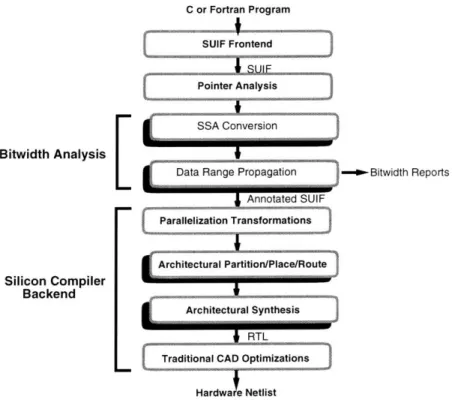
This chapter presents results from a stand-alone Bitwise Compiler. The compiler is composed of the first four steps shown in Figure 6-1. Further results, after processing

with the silicon compiler backend (the last four steps in the flowchart), are presented in Chapter 7.

The frontend of the compiler takes as input a program written in C or FORTRAN and produces a bitwidth-annotated SUIF file. After parsing the input program into

SUIF, the compiler performs traditional optimizations and then pointer analysis [21].

The next two passes, labeled "Bitwidth Analysis", are the realization of the algorithms

discussed in this paper. Here, the SUIF intermediate representation is converted to SSA form, including the extensions discussed in Chapter 4 and Chapter 5. Finally,

the data-range propagation pass is invoked to produce bitwidth-annotated SUIF along with the appropriate bitwidth reports. In total, they comprise roughly 12,000 lines of C++ code. We first discuss the bitwidth reports that are generated after these passes.

6.1

Experiments

The prototype compiler does not currently support recursion. Although this

restric-tion limits the complexity of the benchmarks we can analyze, it provides adequate support of programs written for high-level silicon synthesis.

C or Fortran Program S U IF Frontend Pointer Analysis SSA Conversion Bitwidth Analysis Silicon Compiler Backend

L

Parallelization Transformations

Architectural Partition/Place/Rloute

Architectural Synthesis RTL Traditional CAD Optimizations

Hardwa e Netlist

Figure 6-1: Compiler flow: includes general SUIF, Bitwise, silicon, and CAD processing steps. The raised steps are new Bitwise or DeepC passes, and the remaining steps are re-used from previous SUIF compiler passes.

Benchmark Type Source Lines Description softfloat Emulation Berkeley 1815 Floating Point adpcm Multimedia UTdsp 195 Audio Compress bubblesort Scientific Raw 62 Bubble Sort

life Automata Raw 150 Game of Life intmatmul Scientific Raw 78 Int. Matrix Mult.

jacobi Scientific Raw 84 Jacobi Relation median Multimedia UTdsp 86 Median Filter

mpegcorr Multimedia MIT 144 From MPEG Kernel sha Encryption MIT 638 Secure Hash

bilinterp Multimedia MMX 110 Bilinear Interp. convolve Multimedia MIT 74 Convolution histogram Multimedia UTdsp 115 Histogram intfir Multimedia UTdsp 64 Integer FIR

newlife Automata MIT 119 New Game of Life

parity Multimedia MIT 54 Parity Function pmatch Multimedia MIT 63 Pattern Matching

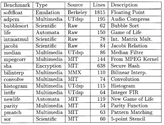
sor Scientific MIT 60 5-point Stencil Table 6.1: Benchmark characteristics

Table 6.1 lists the benchmarks used to quantify the performance of Bitwise. The source code for the benchmarks can be found at [5]. We include several contemporary multimedia applications as well as standard applications that contain predominantly bit-level or byte-level operations, such as life and softfloat.

6.2

Register Bit Elimination

Figure 6-2 shows the percentage of the original register bits remaining in the program after Bitwise has run, while Table 6.2 shows the absolute number of bits saved in a progam. Register bits are used to store scalar program variables. The lower bound - which was obtained by profiling the code - is included for reference. For the particular data sets supplied to the benchmark, this lower bound represents the fewest number of bits needed to retain program correctness. That is, it forms a lower bound on the minimum bitwidth that can be determined by static analysis, which must be correct over all input data-sets. The graph assumes that each variable is assigned to its

own register. However, downstream architectural synthesis passes include a register allocator. If variables with differing bitwidths share the same physical register, the final hardware may not capture all of the gains of our analysis. Our metric is a useful overall gauge because register bitwidths affect functional unit size, data path bitwidths, and circuit switching activity.

Our analysis dramatically reduces the total number of register bits needed. In most cases, the analysis is near optimal, which is especially exciting for applications that perform abundant multi-granular computations. For instance, Bitwise nearly matches the lower bound for life and mpegcorr, which are bit-level and byte-level

applications respectively.

The only applications in the figure with substantially sub-optimal performance compared to the dynamic profile are median and softfloat. In the case of median, the analyzer was unable to determine the bitwidth of the input data, thus variables that were dependent on the input data assumed the maximum possible bitwidths. Although dynamic profiling of softfloat shows plenty of opportunities for bitwidth reduction, these opportunities are specific to particular control flow paths and were not discovered during our static analysis of the whole program.

6.3

Memory Bit Elimination

Figure 6-3 shows the percentage of the original memory bits remaining in the program. Table 6.3 shows the actual number of memory bits in the program both before and after bitwidth analysis. Here memory bits are defined as data allocated for static arrays and dynamically allocated variables. This is an especially useful metric when compiling to non-conventional devices such as an FPGA, where memories may be segmented into many small chunks. In addition, because memory systems are one of the primary consumers of power in modern processors, this is a useful metric for estimating power consumption [12].

In almost all cases, the analyzer is able to determine near-optimal bitwidths for the memories. There are a couple of contributing factors for Bitwise's success in reducing

vith Bitwise E dynamic profile - - - -... 100% -8 0 % - --- -- - --- -60% -40% - - - --- 2 0 % -L 0% % E - -- 5 o C. 0 0. -0 E =3 -C 0 - C0 f CU a) 0 E a0 E -a ' - -- --- - - --i 0 3- (U (U C0 0 UL M 0

Figure 6-2: Percentage of total register bits remaining: post-bitwidth analysis versus dy-namic profile-based lower bound.

array bitwidths. First, many multimedia applications initialize static constant tables which represent a large portion of the memory savings shown in the figure. Second, Bitwise capitalizes on arrays of Boolean variables.

6.4

Bitwidth Distribution

It is interesting to categorize variable bitwidths according to grain size. The stacked bar chart in Figure 6-4 shows the distribution of variable bitwidths both before and

after bitwidth analysis. We call this distribution a Bitspectrum. To make the graph

more coherent, bitwidths are rounded up to the nearest typical machine data-type size. In most cases, the number of 32-bit variables is substantially reduced to 16, 8, and 1-bit values.

For silicon compilation, this figure estimates the overall register bits that can be saved. As we will see in the next chapters, reducing register bits results in smaller datapaths and subsequently smaller, faster, and more efficient circuits.

Benchmark Before Bitwise After Bitwise Dynamic Profile softfloat 2432 1057 391 adpcm 416 137 103 bubblesort 224 78 75 life 576 125 114 intmatmul 256 157 153 jacobi 160 72 57 median 224 129 66 mpegcorr 512 102 78 sha 928 821 800 bilinterp 864 394 380 convolve 64 23 23 histogram 192 131 121 intfir 128 79 68 newlife 192 62 60 parity 128 29 29 pmatch 128 30 21 sor 96 29 28

Table 6.2: The actual number of bits in the progam before and after bitwidth analysis. The dynamic lower bound which was obtained by runtime profiling is included for reference. higher degrees of parallelism [14]. In this context, the spectrum shows which appli-cations will have the best prospect for packing values into sub-word instructions.

E with Bitwise i dyamic profile 100% ---- - - -- ---80% -60% 40% -20% --- - - --0% w bnd CO E 75 Z E'~ 0u 0 E) 0-0 .5 ~ -0 cc M ) C) > ) CD C o cc -0 E E 0 ~ CL E L)

-Figure 6-3: Percentage of total memory remaining: post-bitwidth analysis versus dynamic profile-based lower bound.

Benchmark Before Bitwise After Bitwise Dynamic Profile softiloat 8192 1024 1024 adpcm 118912 38727 21871 bubblesort 32768 16384 16384 life 69632 2176 2176 intmatmul 98304 55296 53248 jacobi 4096 1024 1024 median 131712 131712 103947 mpegcorr 2560 2560 2560 sha 16384 5120 4608 bilinterp 4736 4648 4600 convolve 12800 12544 12544 histogram 534528 135168 133120 intfir 64512 62400 51136 newlife 33792 2048 2048 parity 32768 31744 31744 pmatch 68608 36736 36736 sor 532512 532512 532512

Table 6.3: The actual number of memory bits in the progam before and after bitwidth analysis. The dynamic lower bound which was obtained by runtime profiling is included for reference.

32 bits 1-16 bits bits 111 bit68 100% -80% 60% -40% -

I

softfloat bubblesort intmatmul median

adpcm life jacobi mpegcorr

sha

II

5:E 1: sfs5Z s

convolve intfir parity sor

bilinterp histogram newlife pmatch

Figure 6-4: Bitspectrum. This graph is a stacked bar chart that shows the distribution of register bitwidths for each benchmark. Without bitwidth analysis, almost all bitwidths are 32-bits. With Bitwise, many widths are reduced to 16, 8, and 1 bit machine types, as denoted by the narrower 16, 8, and 1 bit bars.

20 0 I

I

-Benchmark with/without 32-bits 116-bits 8-bits 1-bit softfloat with 186 48 66 181 softfloat without 475 6 0 0 adpcm with 15 24 14 5 adpcm without 43 8 7 0 bubblesort with 0 6 0 1 bubblesort without 7 0 0 0 life with 3 0 6 11 life without 20 0 0 0 intmatmul with 4 4 2 0 intmatmul without 10 0 0 0 jacobi with 2 1 5 0 jacobi without 8 0 0 0 median with 13 9 2 2 median without 13 13 0 0 mpegcorr with 8 0 10 2 mpegcorr without 20 0 0 0 sha with 27 2 1 0 sha without 30 0 0 0 bilinterp with 11 4 16 0 bilinterp without 31 0 0 0 convolve with 0 2 0 0 convolve without 2 0 0 0 histogram with 3 2 2 0 histogram without 7 0 0 0 intfir with 2 1 1 0 intfir without 4 0 0 0 newlife with 1 1 4 0 newlife without 6 0 0 0 parity with 0 1 2 0 parity without 3 0 0 0 pmatch with 0 2 1 1 pmatch without 4 0 0 0 sor with 0 1 2 0 sor without 3 0 0 0

.- . ~

r e

e

n

M

w

-9

n

i

--Chapter

7

Quantifying Bitwise's Performance

Thus far we have shown that bitwidth analysis is a generally effective optimization and that our Bitwise Compiler is capable of performing this task well. We now turn

to a concrete application of bitwidth analysis. We have applied bitwidth analysis to the problem of silicon compilation. This chapter briefly discusses the design of a high-level silicon compiler. We then quantify the impact that bitwidth analysis has

in this context.

7.1

DeepC Silicon Compiler

We have integrated Bitwise with the Deep C Silicon Compiler [3]. DeepC is a research compiler under development that is capable of translating sequential applications, written in either C or FORTRAN, directly into a hardware netlist. The compiler automatically generates a specialized parallel architecture for every application. To make this translation feasible, the compilation system incorporates the latest code optimization and parallelization techniques as well as modern hardware synthesis technology. Figure 6-1 shows the details of integrating Bitwise into DeepC's overall compiler flow. After reading in the program and performing traditional compiler

op-timizations and pointer analysis, the bitwidth analysis steps are then invoked. These

steps were described in detail in Chapters 3 and 4. The additional steps of the silicon compiler backend are as follows. First, loop-level parallelizations are applied, followed