Bayesian inference of chemical reaction networks

(1)

Bayesian inference of chemical reaction networks

by

Nikhil Galagali

B.Tech., Indian Institute of Technology Madras (2007)

S.M., Massachusetts Institute of Technology (2009)

Submitted to the Department of Mechanical Engineering

in partial fulfillment of the requirements for the degree of

Doctor of Philosophy in Computational Science and Engineering

at the

MASSACHUSETTS INSTITUTE OF TECHNOLOGY

June 2016

c

○ Massachusetts Institute of Technology 2016. All rights reserved.

Author . . . .

Department of Mechanical Engineering

February 19, 2016

Certified by . . . .

Youssef M. Marzouk

Associate Professor of Aeronautics and Astronautics

Thesis Supervisor

Accepted by . . . .

Rohan Abeyaratne

Chairman, Department Committee on Graduate Students

(2)

(3)

Bayesian inference of chemical reaction networks

by

Nikhil Galagali

Submitted to the Department of Mechanical Engineering on February 19, 2016, in partial fulfillment of the

requirements for the degree of

Doctor of Philosophy in Computational Science and Engineering

Abstract

The development of chemical reaction models aids system design and optimization, along with fundamental understanding, in areas including combustion, catalysis, elec-trochemistry, and biology. A systematic approach to building reaction network models uses available data not only to estimate unknown parameters, but to also learn the model structure. Bayesian inference provides a natural approach for this data-driven construction of models.

Traditional Bayesian model inference methodology is based on evaluating a mul-tidimensional integral for each model. This approach is often infeasible for reaction network inference, as the number of plausible models can be very large. An alternative approach based on model-space sampling can enable large-scale network inference, but its efficient implementation presents many challenges. In this thesis, we present new computational methods that make large-scale nonlinear network inference tractable. Firstly, we exploit the network-based interactions of species to design improved “between-model” proposals for Markov chain Monte Carlo (MCMC). We then intro-duce a sensitivity-based determination of move types which, when combined with the network-aware proposals, yields further sampling efficiency. These algorithms are tested on example problems with up to 1000 plausible models. We find that our new algorithms yield significant gains in sampling performance, with almost two orders of magnitude reduction in the variance of posterior estimates.

We also show that by casting network inference as a fixed-dimensional problem with point-mass priors, we can adapt existing adaptive MCMC methods for network inference. We apply this novel framework to the inference of reaction models for catalytic reforming of methane from a set of ≈ 32000 possible models and real exper-imental data. We find that the use of adaptive MCMC makes large-scale inference of reaction networks feasible without the often extensive manual tuning that is required with conventional approaches.

Finally, we present an approximation-based method that allows sampling over very large model spaces whose exploration remains prohibitively expensive with

(4)

ex-act sampling methods. We run an MCMC algorithm over model indicators and for each visited model approximate the model evidence via Laplace’s method. Limited and sparse available data tend to produce multi-modal posteriors over the model indicators. To perform inference in this setting, we develop a population-based ap-proximate model inference MCMC algorithm. Numerical tests on problems with around 109 _{models demonstrate the superiority of our population-based algorithm}

over single-chain MCMC approaches. Thesis Supervisor: Youssef M. Marzouk

(5)

Acknowledgments

I want to firstly thank my advisor, Youssef Marzouk, for being a great mentor. His enthusiasm for doing research and the rigor he displays in all his pursuits have been a constant source of inspiration to me. This thesis has been shaped by his many in-puts and I am grateful for his guidance. I would also like to thank Ahmed Ghoniem, William Green, Pierre Lermusiaux, and Habib Najm for serving on my thesis com-mittee. Their questions during the committee meetings made me delve deeper into many of the ideas developed in this thesis.

I also would like to acknowledge the members of the Uncertainty Quantification Lab for sharing a congenial atmosphere to work in. Thank you also to all the friends I have made during stay at MIT. Spending time with friends has definitely made the graduate school experience more enjoyable.

I am grateful for the generous financial support from KAUST Global Research Partnership and BP through the BP-MIT Energy Conversion Program during my graduate studies. I am also thankful to Ms. Leslie Regan for the administrative support.

Finally, I would like to thank my parents and my brother for their love and support over all the years I have spent away from home.

(6)

(7)

List of Figures

2-1 A process model. . . 29

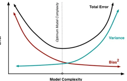
2-2 Bias-variance tradeoff curve . . . 32

3-1 Stagnation flow reactor; figure reproduced from [86].. . . 65

3-2 Reaction networks of the highest posterior probability models for steam reforming of methane (Example 2), under different prior specifications. Edge thicknesses are proportional to reaction rates calculated using posterior mean values of the rate parameters. . . 77

3-3 Posterior reaction inclusion probabilities of all reactions for the three prior specifications in Example 2. The red line indicates the prior reaction inclusion probability. . . 79

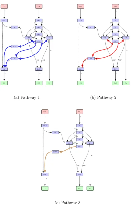
3-4 Reaction pathways for steam reforming of methane on rhodium (Ex-ample 2). Pathway 1 involves both species C* and HCO*, Pathway 2 excludes HCO*, and Pathway 3 excludes C* species. All other re-actions that are treated as uncertain and that do not involve C* and HCO* are dotted. Reactions involving gas-phase species are shown as regular lines.. . . 80

3-5 Reaction networks of the highest posterior probability models for dry reforming of methane (Example 3), under different prior specifications. Edge thicknesses are proportional to reaction rates calculated using posterior mean values of the rate parameters. . . 84

(12)

3-6 Posterior reaction inclusion probabilities of all reactions for the three prior specifications in Example 3. The red line indicates the prior

reaction inclusion probability. . . 86

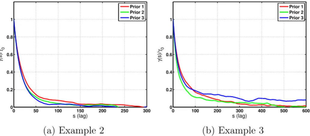
3-7 Reaction pathways for dry reforming of methane on rhodium (Example 3). Pathway 1 involves both species C* and HCO*, Pathway 2 excludes HCO*, and Pathway 3 excludes C* species. All other reactions that are treated as uncertain and that do not involve C* and HCO* are dotted. Reactions involving gas-phase species are shown as regular lines. 87 3-8 Autocorrelation at lag s of the log-posterior of the MCMC chains. . . 88

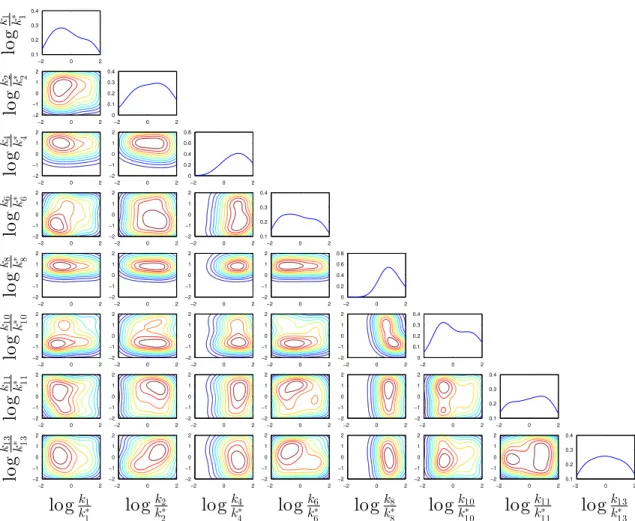
3-9 1-D and 2-D posterior marginals of the rate constants of the highest-posterior-probability model for steam reforming (from Example 2), be-ginning with the prior 𝑝(𝑘𝑖,𝑓) = 0.8𝛿(𝑘𝑖,𝑓) + 0.2𝒞(𝑘𝑖,𝑓). The logarithms here are base 10. . . 90

4-1 A simple reaction network . . . 93

4-2 Common reaction network elements . . . 94

4-3 Reaction network with all reactions . . . 95

4-4 Two reaction networks with the same effective network . . . 97

4-5 Effective reaction network . . . 97

4-6 Efficient RJMCMC: align densities on (𝑘1, 𝑢)to (𝑘2,1, 𝑘2,2)accurately 101 4-7 Model move from network 1 to 2 and 2 to 3 in the standard approach leads to the proposal adapting to the prior. Only the final move from 3 to 4 incorporates the likelihood function . . . 106

4-8 Two networks with different pathways. . . 110

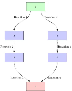
4-9 6 uncertain reactions; species 1 has non-zero initial concentration, species 2, 3, 5, and 6 are produced in operation, and species 4 is observed.117 4-10 Variance of the eight highest posterior model probability estimates in Example 1 . . . 119

(13)

4-11 A reaction network with 5 (reactions 3, 4, 5, 6, and 7) uncertain reac-tions. BRaf is the observable. . . 120

4-12 MCMC trace plots for Example 2: posterior samples from models with both pathways in orange and samples from models with only the left pathway in blue . . . 123

4-13 Variance of the eight highest posterior model probability estimates in Example 2 . . . 125

4-14 MCMC trace plots for Example 2-additional: posterior samples from models with both pathways in orange and samples from models with only the left pathway in blue . . . 127

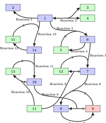
4-15 A reaction network with 6 (reactions 3, 5, 6, 8, 10, and 12) uncertain reactions. BRaf is the observable. . . 128

4-16 MCMC trace plots for Example 3 without sensitivity-based proposals: the generated posterior samples are only from models with both pathways129

4-17 MCMC trace plots for Example 3 with sensitivity-based proposals: posterior samples from models with both pathways in orange and sam-ples from models with only the left pathway in blue . . . 130

4-18 Variance of the eight highest posterior model probability estimates in Example 3 . . . 133

4-19 A reaction network with 10 (reactions 2–12) uncertain reactions. BRaf is the observable. . . 134

4-20 MCMC trace plots for Example 4 without sensitivity-based proposals: the generated posterior samples are only from models with only the left pathway . . . 136

4-21 MCMC trace plots for Example 4 with sensitivity-based proposals: posterior samples from models with both pathways in orange and sam-ples from models with only the left pathway in blue . . . 137

(14)

5-2 Reaction network of Example 2 . . . 154

5-3 Three realizations of single-chain approximate model inference MCMC and population-based approximate model inference MCMC algorithms for Example 2. For the population-based algorithm, we are showing the posterior samples for the chain corresponding to the target distribution ˜

𝑝(𝑀 |𝒟) . . . 157 5-4 Reaction network of Example 3 . . . 158

5-5 Three realizations of single-chain approximate model inference MCMC and population-based approximate model inference MCMC algorithms for Example 3. For the population-based algorithm, we are showing the posterior samples for the chain corresponding to the target distribution ˜

(15)

List of Tables

3.1 Proposed reactions for reforming of methane . . . 70

3.2 Synthetic data sets for Example 1. . . 73

3.3 Proposed reactions for inference in Example 1. . . 74

3.4 The five most probable models and their probabilities, from Example 1. 74 3.5 Experimental operating conditions for Example 2, from [86]. . . 76

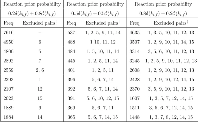
3.6 The ten models with highest posterior probability in Example 2, for each choice of prior.. . . 78

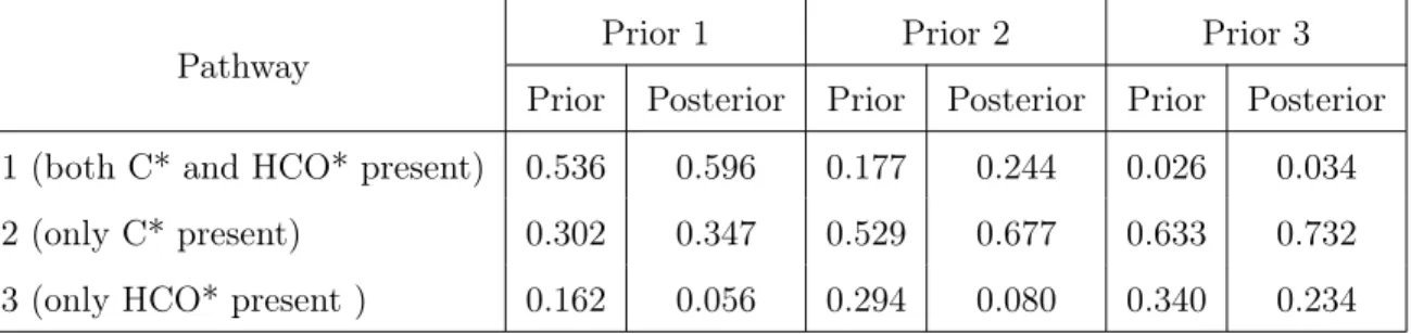
3.7 Prior and posterior pathway probabilities for steam reforming of methane, Example 2. . . 81

3.8 Experimental operating conditions for Example 3 [85]. . . 82

3.9 The ten models with highest posterior probability in Example 3, for each choice of prior.. . . 83

3.10 Posterior pathway probabilities for dry reforming of methane, Example 3. . . 85

4.1 Cluster switching parameter proposals . . . 108

4.2 Summary statistics of MCMC simulations (Example 1). . . 118

4.3 Proposed reactions for Example 2 . . . 122

(16)

5.2 Summary of posterior probabilites for Example 1 by enumeration and sampling . . . 146

5.3 Consistency of posterior probability estimates . . . 148

(17)

Chapter 1 Introduction

1.1 Motivation

Detailed chemical reaction networks are a critical component of simulation tools in a wide range of applications, including combustion, catalysis, electrochemistry, and biology. In addition to being used as predictive tools, network models are also key to developing an improved understanding of the complex process under study. The development of reaction network models typically entails three tasks: selection of participating species, identification of species interactions (refered to as reactions) and the calibration of unknown parameter values. Combustion chemistry has a rich history of building reaction models. Large reaction models with sometimes thou-sands of reactions are well known [28, 67]. In other areas such as systems biology, catalysis, and electrochemistry, the construction of network models can frequently be extremely challenging due to the limited understanding of the operating reaction pathways. For instance, there exist a number of competing hypotheses about H2 and

CO oxidation mechanisms for a solid-oxide fuel cell [62]. Reconstruction of biolog-ical networks involved in cell signalling, gene regulation and metabolism is one of the major challenges in systems biology due to the specificity of species interactions

(18)

[2,17,44, 65]. A standard approach to building models in such a case is to postulate reaction networks and to compare them based on their ability to reproduce indirect system-level experimental data. Data-driven approaches to network learning involve defining a metric of fit, e.g., penalized least-squares, cross-validation, model evidence, etc. and selecting models that optimize this metric. As such, the development of models involves not only the identification of the right model structure, but also the estimation of underlying parameter values given available data.

Bayesian model inference provides a rigorous statistical framework for fusing data with prior knowledge to yield a full description of model and parameter uncertain-ties [13, 46, 111]. The application of Bayesian model inference to reaction networks, however, presents a significant computational challenge. Model discrimination in Bayesian analysis is based on computing model probabilities conditioned on available data, i.e., posterior model probabilities. Formally, the posterior model probability of a model 𝑀𝑛 is given by 𝑝(𝑀𝑛|𝒟) = 𝑝(𝑀𝑛)𝑝(𝒟|𝑀𝑛) ∑︀ 𝑛𝑝(𝑀𝑛)𝑝(𝒟|𝑀𝑛) , where 𝑝(𝒟|𝑀𝑛) = ∫︁ · · · ∫︁ 𝑝(𝒟|𝑘𝑛, 𝑀𝑛)𝑝(𝑘𝑛|𝑀𝑛)𝑑𝑘𝑛

is known as the model evidence, 𝑘𝑛 is the parameter vector of model 𝑀𝑛, and 𝒟

refers to the available data. An approach to Bayesian model inference is to assume that the relationship between species is described by linear or discrete functionals and model parameters take conjugate priors, thereby making the calculation of individ-ual posterior model probabilities analytically tractable. It is, however, often widely believed that species interactions are more appropriately defined by the law of mass action. The law of mass action gives the rate of a chemical reaction (say 𝑋 +𝑌 → 𝑍) as the product of a reaction-specific rate constant 𝑘 with reactant concentrations [𝑋]

(19)

and [𝑌 ]:

Rate = −𝑘[𝑋][𝑌 ]. (1.1)

Under quasi-steady-state assumptions, the law of mass action produces reaction rate expression for enzymatic reactions that are known as Michaelis-Menten functionals [91]. The reaction rate for an enzyme 𝐸 binding to a substrate 𝑆 to produce product 𝑃 (𝐸 + 𝑆 → 𝐸 + 𝑃 ) by Michaelis Menten kinetics is given by

Rate = 𝑘𝑐𝑎𝑡[𝐸]0

[𝑆] 𝑘𝑀 + [𝑆]

, (1.2)

where 𝑘𝑐𝑎𝑡 denotes the rate constant, [𝐸]0 is the enzyme concentration, [𝑆] the

sub-strate concentration, and 𝑘𝑀 the Michaelis constant. Using the law of mass

ac-tion to define reacac-tion rate produces a system of differential equaac-tions such that the parameter-to-observable map (forward model) is typically nonlinear. These equations can be further embedded into differential equation models that describe convective and diffusive transport, surface interactions, and other physical phenomena that af-fect experimental observations. Rigorous computation of posterior model probabilities then requires evaluation of a high-dimensional integral for each model. A number of sampling-based methods exist in the literature for this purpose [26,47,94], but they are computationally taxing. When the number of competing models becomes large, the above methods actually become computationally infeasible.

Reaction network inference is particularly prone to this difficulty, since the number of plausible models can grow exponentially with the number of proposed reactions. A systematic approach to network inference requires appraising a combinatorially large number of models: instead of a few model hypotheses, one might start with a list of proposed reactions, for example, and form a collection of plausible models by consid-ering all valid combinations of the proposed reactions. Alternatives such as Laplace’s method and Bayesian information criterion have been suggested [21,82,109], but they involve approximations of the posterior distribution. Across-model sampling offers a

(20)

solution in cases where the number of models is large [24, 57, 73]. These methods work by making the sampler jump between models to explore the joint posterior dis-tribution over models and parameters. Model probabilities are estimated from the number of times the sampler visits each model. The prohibitively high cost of model comparisons based on the computation of evidence for each model is avoided as the sampler visits each model in proportion to its posterior probability. Efficient across-model sampling, however, is challenging and require a delicate design of proposals for between-model moves. Many practical applications of across-model sampling meth-ods have relied on pilot posterior explorative runs to get a rough idea of the posterior distribution, although a few automated methods do exist in literature [56, 110]. The effective use of across-model sampling methods continues to be a challenge, especially for problems where the parameter-to-observable map is nonlinear.

1.2 Background on reaction network inference

The general problem of network inference has been tackled in the past with various modeling choices and inferential approaches. The modeling of species interactions has spanned from simple Boolean networks to detailed physics-based differential equations and stochastic models. The Boolean network approach relies on simple ON/OFF switches and standard logic interactions to describe species interactions. Additive linear or generalized linear models take an intermediate approach in terms of com-plexity and reliability. The differential equations based network interactions are at the other end of the complexity spectrum, but being rooted in mechanistic models hold the promise of better understanding and improved predictions. From an algo-rithmic standpoint, a large number of inference methods, both from a Bayesian and a non-Bayesian standpoint, have been proposed. We review here a few network in-ference approaches and refer the readers to some detailed reviews for the complete story [44, 96, 98].

(21)

1.2.1 Non-Bayesian reaction network inference

Many non-Bayesian methods for network inference have been published in the chemi-cal and biologichemi-cal engineering literature. Gardner et al. adopted an ODE formulation and developed a technique known as Network Identification by Multiple Regression (NIR) [43]. Their approach constructs a first-order model of regulatory interactions and uses multiple linear regression to infer species interactions. Bansal et al. developed an algorithm known as the Time Series Network Identification in which they assumed a linear ODE model for species interactions and inferred the network topology by a combination of interpolation and principal component analysis [10]. Bonneau et al. use L1 shrinkage to identify transcriptional influences on genes based on the integra-tion of genome annotaintegra-tion and expression data [18]. Margolin et al. have proposed another technique called ARCANE that adopts an information-theoretic approach in which they identify candidate interactions by estimating pairwise species mutual information [84]. Nachman et al. utilize dynamic Bayesian network models and the structural EM algorithm for network identification [92]. Another technique, correla-tion metric construccorrela-tion, suggested by Arkin et al. is based on the calculacorrela-tion and analysis of a time-lagged multivariate correlation function of a set of time-series of chemical concentrations [7]. Burnham et al. propose a statistical technique relying on t-statistics and 𝑅2 _{for the inference of chemical reaction networks governed by}

ordinary differential equations [22].

1.2.2 Bayesian reaction network inference

The Bayesian approach to network inference has seen increasing applications in ar-eas such as protein signalling modeling, gene regulation reconstruction, combustion chemistry etc. The inference methods for signalling topologies and gene regula-tion pathways have principally been developed with linear or discrete formularegula-tions [40, 90,107, 116]. Using Gaussian or multinomial likelihood functions and conjugate priors with these formulations leads to model evidence being available in closed form.

(22)

In spite of the cheap analytical evaluation of evidence, the exponential explosion of the number of networks given species and their possible interactions precludes direct enumeration of model evidence. Thus, sampling based approaches have been devel-oped for large-scale network inference in such contexts [37, 39]. At the same time, ODE-based species interaction models (mass-action kinetics) are also being incorpo-rated into inference frameworks. The use of ODE-based forward models oftentimes results in nonlinear parameter-observable dependency—network inference then has to be based on the computation of model evidence numerically. Xu et al. applied Bayesian model inference with nonlinear ODEs for the elucidation of ERK signalling pathway [118]. Braman et al. used Bayesian methodology for the comparison of syngas chemistry models [19]. However, the methods used above for numerical com-putation of evidence are limited to applications with a small number of hand-crafted models. Large-scale network inference with nonlinear forward models has seen very limited work. Oates et al. applied Bayesian model selection for the comparison of systematically generated models derived from ODE-based species interactions [95]. They used reversible-jump Markov chain Monte Carlo algorithm, a general across-model sampling method, for the simultaneous sampling of network topologies and their underlying parameters. As discussed in 1.1, the use of vanilla across-model sampling methods are generally known to perform poorly. There is a need for the development of efficient large-scale network inference methods that would allow a systematic comparison of exponentially large number of networks, but one that in-corporates nonlinear forward models emerging from ODE-based species interaction formulations.

1.3 Thesis contributions

In this thesis, we present methods for efficient large-scale Bayesian inference of non-linear chemical reaction networks. We develop algorithms that exploit structural

(23)

properties of chemical reaction networks to improve exploration of posteriors over a large number of reaction networks in comparison to existing methods. Further, we develop a model-space sampling approach that makes approximations of the pa-rameter posterior, and thereby allows sampling over very large model spaces whose exploration remains intractable with exact sampling methods.

More specifically, we operate in the across-model sampling framework and make four contributions:

1. Network inference with adaptive MCMC

The rate of a chemical reaction is given by the law of mass action and the net species production rate a species is given by the species production rate from all reactions [77]. The species production rates further feed into forward models that describe convective and diffusive transport, surface interactions, and other phenomena affecting experimental obsevations. Nevertheless, the additive structure of the net species production rate means that reaction inclu-sion/exclusion can be controlled by setting the rate constants to non-zero/zero values. In spite of the overall nonlinear dependency of the observables on the rate constants. This indirect control of network topology by assigning specific values to the rate constants means that the plausible networks are statistically nested. Nested models provide a natural between-model move construction. Nested models can further allow the use of fixed-dimensional Markov chain Monte Carlo (MCMC) algorithms. Adaptive MCMC in which the parameter proposals adapt to posterior samples are known for fixed-dimensional MCMC algorithms and improve sampling efficiency without manual tuning. We exploit the nested structure of reaction network problems and develop an adaptive MCMC algorithm for network inference. The developed algorithm is used to learn reaction networks for steam and dry catalytic reforming of methane on rhodium from a set of 15 proposed reactions and real experimental data. 2. Network-aware sampling

(24)

Chemical reaction networks can quickly become very complex [28, 108]. The network of species interactions, however, has a special structure hidden in it. The production/destruction of a species is directly linked to the concentration of other species it is participating in a reaction with. Therefore, the rate of production/destruction of a species will necessarily be zero if those other species are absent from the system. From a data-analytic perspective, the available data cannot inform the presence of reactions with zero reaction-rate. Many species in a reaction network such as catalysts or enzymes play a fundamental role in the operation of reactions, but do not get consumed. Moreover, practically feasible experiments yield data that is sparse—data is only linked to a few of the species. Sparsity of data and presence of catalyst/enzymes can further render some reactions ineffective in influencing the observables. Thus, the inclusion of these reactions is also not informed by data. We develop a network-aware across-modeling sampling algorithm that recognizes the effective networks being inferred and exploits this knowledge to design efficient parameter proposals for moves between models. This translates into superior sampling performance and low-variance posterior estimates. The recognition of effective networks also allows derandomization of some conditional expectations and thereby yields further variance reduction.

3. Sensitivity-based network-aware sampling

Not all reactions in a network are equally important in influencing the observ-ables. The identification of reactions that have a sharper impact on observables can be critical in designing improved across-model samplers. We develop a local sensitivity-based metric to identify key reactions and use this to develop better between-model move proposals for the reversible jump MCMC algorithm. Com-bining the sensitivity-based proposal construction along with network-aware sampling produces a highly improved nonlinear network inference algorithm. We apply the algorithm for the inference of network topology from a set of 1024

(25)

systematically generated networks that were obtained from a subset of proposed reactions for the activation of the extracellular signal-regulated kinase pathway by epidermal growth factor [118].

4. Network inference with approximation

The network inference methods in Contributions 1, 2, and 3 are exact sampling methods, i.e., they are guaranteed to converge to the correct posterior distri-bution asymptotically as sampling proceeds. Exact inference methods over the joint space of models and parameters are essential for consistency of poste-rior estimates and their development is an important goal. However, for very large model spaces, exact sampling may still be very expensive. We develop an approximation-based network inference approach by using Laplace’s method to approximate model evidences and using Markov chain Monte Carlo to ex-plore the posterior distribution only over model indicators. Nonlinearity of the forward model and limited available data results in the posterior distribution over models being multimodal. To explore multimodal posterior distributions, we extend the approximate posterior inference to a population-based network inference algorithm. The developed algorithm is then used to infer signalling networks from a space of 109 _{plausible networks.}

This thesis is organized into 6 chapters. Following the introduction in Chapter 1, Chapter 2 gives a detailed overview of the motivations for model inference, contrasts different model inference approaches, highlights Bayesian model inference, and dis-cusses existing numerical methods for Bayesian model inference. Chapters 3, 4, and 5 present the four main contributions of this thesis. We summarize and discuss future work in Chapter 6.

(26)

(27)

Chapter 2 Model inference: formulation and

numerical approaches

An integral component of scientific research is the construction of models for the physical process under study. Models are created for two main reasons: they enable an easy understanding of a complex process by breaking it down into more readily interpretable modules, and models can be used for making predictions of unobserved quantities. Development of reliable models is often very hard because one may only get to observe a few noisy realizations of the physical process—referred to as data. Utilizing the available data and any background information about the process, the job of a model developer is to construct a consistent set of equations that relate the model inputs and model parameters to the quantities of interest. Historically, models have been built by empiricism and experimental investigation. More recently, first-principles calculations have also been used to aid model development in disciplines such as chemistry and biology. However, the development of faster computers and the availability of high-quality data has now allowed the use of rigorous statistical techniques in the model development phase. Given a set of plausible models and some data, tools from statistical inference can be used for a systematic evaluation of all models to identify the “best” set of models. In this chapter, we discuss the

(28)

motivations for model inference, present a popular philosophy for effective learning of models from data, outline common approaches for model inference, introduce the Bayesian paradigm for model learning, and discuss some numerical techniques for Bayesian model inference.

2.1 Model inference

Model inference can be defined informally as the assessment of models to ascertain the degree to which each is supported by available data. A prerequisite for model inference is the availability of (i) plausible models and (ii) relevant data to discriminate among the models. Very often, we also have a great deal of background information about the quality of competing models and the values of their underlying parameters. This knowledge—termed as prior information—can be incorporated in the model inference framework. It is important at this stage to distinguish model inference from the common practice of model reduction in chemical kinetics [14,97]. Model reduction refers to a systematic reduction in the size of a large kinetic model so as to reproduce model outputs within a specified tolerance. Such a procedure, however, assumes that an accurate model (i.e., the full kinetic model) is already known and fixed. And, crucially, it does not take experimental data into account during reduction.

A model of a physical process describes a specific collection of input-output re-lationships. In particular, a model describes how some pre-specified quantities of interest are related to input variables. As a result, a model may preclude the de-scription of quantities for which it has not been specifically built. Figure2-1 shows a typical process model. This model—consisting of governing equations expressing con-servation laws, reaction network models, and thermo-kinetic parameters—may relate inputs such as concentration 𝐶𝑖𝑛, temperature 𝑇𝑖𝑛, pressure 𝑃 , and applied voltage

(29)

Inputs

C𝑖𝑛/T𝑖𝑛/P/ΔV

Process model governing equations reaction network model

parameters

Quantities of interest C𝑜𝑢𝑡/t𝑖𝑔𝑛/I

Figure 2-1: A process model

2.2 Goals of model inference

To be able to prescribe a set of rules that determine the best or the most likely model, we need to precisely define the purpose of model inference. Model inference is performed primarily for two purposes: interpretation and prediction. Frequently, the models being compared during inference are physics-based. In such cases, the selected model can be used to gain valuable insight into the operating mechanism. This kind of insight is often used for experimental design. The other main objective of model inference is to make predictions of the quantities of interest.

The selection of the best model based on available data and prior information is essentially a statistical problem. As the amount of data grows, the precision of inference improves and our confidence in the selected model grows. However, in most practical situations, the amount of data required to strongly discriminate between models is unavailable. This engenders significant uncertainty in the inferred results. Thus it is imperative—for reliable inference and accurate quantification of prediction uncertainties—that the model inference method provide means to quantify model uncertainty.

In the next section, we discuss commonly used criteria for model inference and highlight Occam’s razor, which is a powerful approach for model discrimination based on the intuitive idea of balancing model fit with complexity.

(30)

2.3 Approaches for model inference

Having presented a few motivations for model inference, we now proceed to discuss three approaches for model choice. Since the data we would be using to infer the best model will necessarily be noisy, it would be incorrect to try to fit exactly to all available data. If we maximize the quality of fit to the available data, it is the most complex model—model with the largest degrees of freedom—which typically would best fit the data. As we discuss in the following paragraphs, such a strategy would be sub-optimal since the objective is to select models that peform well for all data, not just the observed data.

2.3.1 Model selection based on estimation of prediction error

Model inference is sometimes performed in a data rich situation. In such settings, the available data can be used to compute an estimate of prediction error known as the empirical prediction error [64]. To begin with, the available data is split into three parts: a training set, a validation set, and a test set. The training set is used to fit the models; the validation set is used to estimate the prediction error for model selection; the test set is used for the assessment of the generalization error of the final chosen model. In a slightly data deficient situation, test set can be used to select the model as well as estimate the prediction error. In such cases, the final chosen model will necessarily underestimate the prediction error [64].

2.3.2 Cross validation

Cross-validation is another method that is used often to estimate the prediction error. A 𝐾-fold cross-validation procedure begins by splitting the available data into 𝐾 sets. Then a model is trained using data from 𝐾 − 1 sets as the training data and the prediction error computed on the 𝐾th set as the test set. This process is repeated for all 𝐾 sets and then the average prediction error computed. By performing these

(31)

operations for all 𝑀 competing models, one can select the most well supported model or rank the competing models. Mathematically, we let 𝑠 : {1, ..., 𝑁}| → {1, ..., 𝐾} be an indexing function that indicates the partition to which data point 𝑛 is allotted. We denote by ˆ𝑓−𝑠(𝑥) the fitted function, computed with the 𝑠𝑡ℎ _{part of the data}

removed. Then the cross-validation estimate of the prediction error is 𝐶𝑉 = 1 𝑁 𝑁 ∑︁ 𝑛=1 𝐿(𝑦𝑛, ˆ𝑓−𝑠(𝑛)(𝑥𝑛)) (2.1)

When 𝐾 = 𝑁, the cross-validation method is referred to as leave-one-out cross vali-dation [64].

2.3.3 Goodness-of-fit and complexity penalty

A well known observation pertaining to the fitting of model parameters to available data is that the goodness-of-fit generally improves as the model complexity grows. Though the mismatch between model predictions and available data decreases as the model complexity increases, we would not expect our future predictions to be very accurate. This is because by increasing model complexity we begin to fit to the noise in the data. This problem is known as the problem of overfitting in statistics. Thus, a common strategy is to adopt a model inference criterion such that the mismatch between model predictions and available data is agreeable and at the same time model complexity is limited. This two-fold objective is also described by the bias-variance tradeoff [64]. As the complexity of the model grows, the variance of the inferred parameters would be high, and as a result, the expected prediction error of the model tends to be high. On the contrary, simpler models tend to have higher bias, and so fit poorly to available data and have high prediction error (Figure 2-2).

The best models tend to be ones that balance bias with variance. Therefore, a popular approach to model selection is one that rewards good agreement with available data, but also penalizes model complexity. This guiding principle for the

(32)

Figure 2-2: Bias-variance tradeoff curve

assessment of models, first suggested by William of Ockham, is encapsulated by the Occam’s razor [82]. The Occam’s razor principle is suitable irrespective of whether the objective model inference is interpretation or prediction. The explanation for prediction is clear from the discussion from the last paragraph. Even in cases where the goal of model inference is interpretation, it makes sense that we determine model strength not just based on fit to available data. In this thesis, we work with methods that balance bias with variance. In such cases, the key is to determine the penalty term that would penalize model complexity appropriately.

2.4 Balancing goodness-of-fit with model complexity

The goal of this section is to discuss methods that balance the quality of fit to available data with the complexity of the fitted model. The cross-validation (CV) method presented in the last section is most suitable when the amount of available data is plentiful [8, 64]; in a data-poor context, the cross-validation metric is noisy and its results highly variable. A method that explicitly incorporates an Occam’s razor is more useful for the data-deficient case one typically encounters in reaction network inference.

(33)

In statistics in general, there are two main viewpoints for the identification of likely models and their underlying parameter values from data. The frequentist ap-proach to learning treats the models and parameters as fixed unknown quantities that are determined by techniques that aim to produce good estimation over all possible data sets. The Bayesian approach, in contrast, regards the models and parameters as random variables whose distributions conditioned on available data are determined by the consistent application of the rules of probability theory. Model selection ap-proaches in the frequentist setting, such as 𝐶𝑝-statistic, Akaike information criterion,

etc, impose an Occam’s razor by selecting models based on the following optimization problem:

𝑀* = arg min

𝑀

||𝒟 − 𝐺𝑀(𝑘𝑀)|| + 𝛼|𝑀 |,

where 𝑀* _{is the optimal model, 𝐺}

𝑀 is the prediction with model 𝑀, 𝑘𝑀 are the

parameters of model 𝑀, 𝒟 the observed data, ||𝒟 − 𝐺𝑀(𝑘𝑀)|| is the data misfit,

|𝑀 |is the model complexity, and 𝛼 is the penalty on model complexity. The problem with the above optimization based approaches is that they tend to be ad hoc, due to a lack of a clear guideline about the right value for the penalty 𝛼 [12].

2.5 Bayesian approach to model inference

Bayesian statistics provides a rigorous inference framework to assimilate noisy and indirect data, a natural mechanism to incorporate prior knowledge from different sources, and a full description of uncertainties in parameter values and model struc-ture. It is based on Bayes’ rule of probability:

𝑝(𝑘|𝒟) = 𝑝(𝒟|𝑘)𝑝(𝑘)

(34)

Here, 𝑘 is the parameter being inferred, 𝑝(𝑘|𝒟) is the posterior probability den-sity of 𝑘 conditioned on data 𝒟, 𝑝(𝒟|𝑘) is the likelihood of observing 𝒟 given the parameter value, and 𝑝(𝑘) is the prior probability density of parameter 𝑘. 𝑝(𝒟), commonly refered to as evidence or marginal likelihood, is the marginal distribution of data. Sampling the posterior enables description of posterior uncertainty and the estimation of posterior summaries such as the mean and standard deviation. Posterior exploration by sampling is seldom directly feasible except for conjugate prior distri-butions. For nonlinear forward models and/or non-conjugate prior distributions, one has to rely on an indirect sampling approach, such as importance sampling or Markov chain Monte Carlo [3, 51]. Application of Bayesian parameter inference to physical models has received much recent interest [9, 74, 89, 113], with applications ranging from geophysics [35, 55] and climate modeling [71] to reaction kinetics [53, 78,99].

Applying Bayes’ rule to models 𝑀, we get

𝑝(𝑀 |𝒟) = 𝑝(𝒟|𝑀 )𝑝(𝑀 )

𝑝(𝒟) . (2.3)

Comparing the posterior of any two models, 𝑀𝑖 and 𝑀𝑗, yields the posterior odds:

𝑝(𝑀𝑖|𝒟)

𝑝(𝑀𝑗|𝒟)

= 𝑝(𝒟|𝑀𝑖)𝑝(𝑀𝑖) 𝑝(𝒟|𝑀𝑗)𝑝(𝑀𝑗)

(2.4) Assuming that all models are equally probable before the observation of data, we get

𝑝(𝑀𝑖|𝒟)

𝑝(𝑀𝑗|𝒟)

= 𝑝(𝒟|𝑀𝑖) 𝑝(𝒟|𝑀𝑗)

. (2.5)

The quantity on the right-hand side of Equation 2.5 is known as Bayes factor and is the traditional metric used to compare the probabilities of different models [13, 46,

75]. A key advantage of this Bayesian formulation is an implicit penalty on model complexity in the model evidence—an automatic Occam’s razor that guards against overfitting [82]. Computation of Bayes factor, however, is expensive as it relies on the evaluation of high-dimensional integrals. Specifically,

(35)

𝑝(𝒟|𝑀𝑖)

𝑝(𝒟|𝑀𝑗)

= ∫︀ 𝑝(𝒟|𝑘𝑖)𝑝(𝑘𝑖|𝑀𝑖)𝑑𝑘𝑖 ∫︀ 𝑝(𝒟|𝑘𝑗)𝑝(𝑘𝑗|𝑀𝑗)𝑑𝑘𝑗

(2.6) where 𝑘𝑖 and 𝑘𝑗 are model-specific multidimensional parameters. Alternatives such

as Laplace approximation method and Bayesian information criterion have been sug-gested in the literature [21, 82, 109], but they all involve making approximations about distributions. The standard approach presented above becomes infeasible for an exhaustive comparison of a large number of models because of the high computa-tional cost involved. As mentioned in Chapter1, in this thesis, we focus on developing tractable network inference methodologies when the number of plausible models is large. The underlying rate parameter uncertainties would come “for free" as a natural byproduct of the model inference results.

The Bayesian posterior model probabilities also have the advantage of being eas-ily interpretable. Having computed the posterior probabilities of the models, it is straightforward to understand the degree to which the different models are supported by available data based on their posterior probabilities. The Bayesian model inference procedure has another favorable property in that it is consistent. Consistency is a property that if the true model is among the set of models being compared, then the posterior probability of the true model converges to 1 in probability as the size of the data set goes to infinity.

2.6 Numerical methods for Bayesian computation

The generation of samples from posterior distributions is a central problem in Bayesian statistics. Integration of functions with respect to posterior distributions in high-dimensions is most efficiently performed by Monte Carlo sampling. Formally, the

(36)

posterior distribution can be defined over a general state space Θ ∈⋃︁

𝑀

{𝑀 } × 𝑘𝑀, (2.7)

where 𝑘𝑀 ⊆ R𝑀 are parameter spaces and each parameter space 𝑘𝑀 could have a

different dimensionality. 𝑀 here acts as an indicator of the individual parameter spaces. The posterior distribution over Θ is again given by Bayes’ rule:

Note, in relation to models and parameters discussed in the previous section, 𝑀 would correspond to model indicators and 𝑘𝑀 then are their respective parameter vectors.

The posterior distribution over 𝑀 and 𝑘𝑀 are related through a marginalization:

𝑝(𝑀 |𝒟) = ∫︁

𝑘𝑀

𝑝(𝑀, 𝑘𝑀|𝒟) (2.9)

When the forward model is nonlinear or the prior distributions are non-conjugate, the sampling of the posterior distribution 𝑝(Θ|𝒟) using standard Monte Carlo is infeasible. In such cases, one has to resort to advanced Monte Carlo methods, the most widely useful of which are a general class of algorithms known as the Markov chain Monte Carlo methods.

In the following sections, we discuss various Monte Carlo methods that enable computation of posterior model probabilities and in many cases also produce samples from parameter posterior distributions. We begin with a brief discussion of an algo-rithm used for fixed-dimensional posterior sampling known as the Metropolis-Hastings algorithm.

(37)

2.6.1 Metropolis-Hastings algorithm

In many problems of interest, the model structure is assumed to be well known. Thus the target of the inference procedure is only the posterior distribution over the underlying parameters of the model. Sampling in such a fixed-dimensional setting, when direct sampling is infeasible, is commonly performed using the Metropolis-Hastings algorithm. The Metropolis-Metropolis-Hastings algorithm is an iterative algorithm that produces a Markov chain whose limiting distribution is the posterior distribution 𝑝(𝑘|𝒟). At each step of the algorithm, a sample from a distribution 𝑞(𝑘|𝑘𝑛) known as the proposal distribution is generated. The proposed sample is accepted as the new state of the chain with a probability that depends on the posterior and proposal distributions. If the proposed sample is rejected, the current state of the chain is retained as the new state. The steps of the Metropolis-Hastings algorithm are given in Algorithm 1.

Algorithm 1 The Metropolis-Hastings algorithm

1: Given: Data 𝒟, prior density 𝑝(𝑘), likelihood function 𝑝(𝒟|𝑘), proposal density

𝑞(𝑘|𝑘𝑛₎_{, number of steps 𝑁} 2: Initialize 𝑘0 3: for 𝑛 = 0 to 𝑁 − 1 do 4: Sample 𝑢 ∼ 𝒰_[0,1] 5: Sample 𝑘* ∼ 𝑞(𝑘|𝑘𝑡) 6: if 𝑢 < 𝛼(𝑘𝑡, 𝑘*) = min {︁ 1,𝑝(𝑘_𝑝(𝑘*𝑡_{|𝒟)𝑞(𝑘}|𝒟)𝑞(𝑘*𝑡|𝑘_|𝑘*𝑡)₎ }︁ then 7: 𝑘𝑛+1_{= 𝑘}* 8: else 9: 𝑘𝑛+1= 𝑘𝑛 10: end if 11: end for

Under mild conditions, the above algorithm guarantees convergence of the distribution of the Markov chain state 𝑘𝑛 _{to the posterior distribution and the existence of limit}

(38)

¯ 𝑓 = 1 𝑁 𝑁 ∑︁ 𝑛=1 𝑓 (𝑘𝑛). (2.10)

that converges almost surely to ∫︀ 𝑓(𝑘)𝑝(𝑘|𝒟)𝑑𝑘 by the strong law of large numbers. In contrast to standard Monte Carlo sampling, the sequence of iterates produced by the Metropolis-Hastings algorithm are correlated and thus the posterior estimates have a higher variance. Special cases of the general Metropolis-Hastings algorithm are obtained by considering specific choices of the proposal distribution 𝑞(𝑘|𝑘𝑛₎. If the

proposal is independent of the current location of the chain, we get the Independence Metropolis-Hastings algorithm. Another very popular algorithm is obtained by con-sidering proposals that consist of independent perturbations about the current state. Specifically, the proposal is of the form 𝑘* _{= 𝑘}𝑛_{+ 𝜖}

𝑛, where 𝜖𝑛 ∼ 𝑞is independent of

𝑘𝑛_{. The resulting algorithm is then known as the random-walk Metropolis-Hastings}

algorithm.

2.6.2 Computing the posterior model probabilities

The evaluation of posterior model probabilities in the Bayesian framework is often a challenging computational problem. The computation of model evidence is seldom analytically tractable. When the forward model is linear, the use of conjugate priors permits closed form solutions for model evidence. However, in many practical sit-uations, we encounter a nonlinear parameter-observable dependency. The evidence is then obtained by resorting to numerical techniques. Formally, the objective is to approximate the posterior model probability distribution 𝑝(𝑀|𝒟). For any model 𝑀𝑖,

𝑝(𝑀𝑖|𝒟) ∝ 𝑝(𝒟|𝑀𝑖)𝑝(𝑀𝑖), (2.11)

(39)

𝑝(𝒟|𝑀𝑖) =

∫︁

𝑝(𝒟|𝑘𝑖, 𝑀𝑖)𝑝(𝑘𝑖|𝑀𝑖)𝑑𝑘𝑖, (2.12)

and 𝑝(𝑀𝑖) is the prior probability of model 𝑀𝑖 and 𝑘𝑖 is the vector of unknown

paramters in model 𝑀𝑖. The computation of the above multidimensional integral

is carried out by numerical methods. In low-dimensional settings, it is sometimes efficient to compute the integral by numerical quadrature schemes [29, 48]. But for moderate to high-dimensional integrals, sampling-based methods are necessary. We provide a brief overview of some of the commonly used sampling-based methods for Bayesian model inference.

2.6.3 Computing the evidence via model-specific Monte Carlo

simulations

Many existing methods in literature compute posterior model probabilities by esti-mating the model evidence (2.12) individually for all competing models.

Standard Monte Carlo and importance sampling

A simple approach to estimating the model evidence for a model 𝑀𝑖 is to evaluate

the Monte Carlo sum by sampling from the prior distribution 𝑝(𝑘𝑖). The estimate

ˆ 𝑝(𝒟|𝑀𝑖) = 1 𝑁 𝑁 ∑︁ 𝑛=1 𝑝(𝒟|𝑘𝑛_𝑖), (2.13) where 𝑘𝑛

𝑖 ∼ 𝑝(𝑘𝑖), is guaranteed to converge almost surely to the true model evidence

by the strong law of large numbers [105]. Although very simple, this approach is highly inefficient as most samples are drawn from regions of the parameter space where the likelihood tends to have a low value. Practically, this manifests into high variance in evidence estimates.

An improvement to the above estimator is to use importance sampling. Impor-tance sampling involves generating samples from a different distribution 𝑞(𝑘𝑖)known

(40)

as the proposal. Under some general conditions, a simulation consistent estimate is given by ˆ 𝑝(𝒟|𝑀𝑖) = 1 𝑁 𝑁 ∑︁ 𝑛=1 𝑤𝑛𝑝(𝒟|𝑘𝑛_𝑖) (2.14)

where 𝑤𝑛= 𝑝(𝑘𝑛_𝑖)/𝑞(𝑘_𝑖𝑛)and 𝑘𝑛_𝑖 ∼ 𝑞(𝑘𝑖)[49]. The precision of importance sampling

estimates hinges on 𝑞(𝑘𝑖) being a good approximation of 𝑝(𝑘𝑖|𝒟) and thus good

proposal distributions 𝑞(𝑘𝑖)are a priori hard to design in complex multi-dimensional

settings.

Posterior harmonic mean estimator

Newton et al. [94] suggested another importance sampling estimator for the estimation of model evidence. In contrast to the standard importance sampling estimator (2.14), an alternative simulation consistent importance sampling estimator is given by

ˆ 𝑝(𝒟|𝑀𝑖) = ∑︀𝑁 𝑛=1𝑤𝑛𝑝(𝒟|𝑘𝑛_𝑖) ∑︀𝑁 𝑛=1𝑤𝑛 . (2.15) Here again 𝑤𝑛 = 𝑝(𝑘𝑛𝑖)/𝑞(𝑘 𝑛 𝑖) and 𝑘 𝑛

𝑖 ∼ 𝑞(𝑘𝑖) [49]. The advantage of this estimator

is that the proposal need only be known upto an unknown constant. Newton et al. [94] noted that the posterior distribution 𝑝(𝑘𝑖|𝒟) is an efficient proposal distribution

and if we simulate samples approximately from the posterior, substitution into (2.15) yields an estimate of 𝑝(𝒟|𝑀𝑖), ˆ 𝑝(𝒟|𝑀𝑖) = {︃ 1 𝑁 𝑁 ∑︁ 𝑛=1 𝑝(𝒟|𝑘𝑛_𝑖)−1 }︃−1 , (2.16)

called the harmonic mean estimator. The simulation of posterior samples may be performed by Markov chain Monte Carlo or sequential-importance-resampling meth-ods [3]. It can easily be verified that the estimator (2.16) converges almost surely to the correct model evidence. The drawback of the harmonic estimator is that it

(41)

can be unstable because 𝑝(𝒟|𝑘𝑖)−1 is often not square integrable with respect to the

posterior distribution.

Marginal likelihood from the Gibbs and the Metropolis-Hastings output Another set of approaches proposed by Chib [25] and Chib et al. [26] involves expand-ing the model evidence in terms of the likelihood, prior, and the posterior density at a parameter value 𝑘*

𝑖 and then estimating the posterior density value at 𝑘 *

𝑖 using

sam-ples generated from the posterior distribution. The evidence being the normalizing constant is given by

𝑝(𝒟|𝑘*_𝑖)𝑝(𝑘*_𝑖)

𝑝(𝑘_𝑖*|𝒟) . (2.17)

If ˆ𝑝(𝑘*

𝑖|𝒟) is a posterior estimate, then the estimate of model evidence on the

loga-rithm scale is

log ˆ𝑝(𝒟|𝑀𝑖) = log 𝑝(𝒟|𝑘*_𝑖) + log ˆ𝑝(𝑘*_𝑖) − log ˆ𝑝(𝑘_𝑖*|𝒟). (2.18)

When the posterior conditionals 𝑝(𝑘𝑖|𝒟, 𝑧) and 𝑝(𝑧|𝒟, 𝑘𝑖) are available, Chib [25]

propose using the output from the Gibbs sampler {𝑘𝑛 𝑖 , 𝑧

𝑛_}𝑁

𝑛=1 to obtain a Monte

Carlo estimate of 𝑝(𝑘𝑖|𝒟) =∫︀ 𝑝(𝑘𝑖|𝒟, 𝑧)𝑝(𝑧|𝒟)𝑑𝑧 given as

ˆ 𝑝(𝑘_𝑖*|𝒟) = 𝑁−1 𝑁 ∑︁ 𝑛=1 𝑝(𝑘*|𝒟, 𝑧𝑛_). _(2.19)

Chib et al. [26] extend the method to cases when full conditionals are intractable and posterior samples are simulated using the Metropolis-Hastings algorithm. If {𝑘𝑛

𝑖} 𝑁 𝑛=1

are samples from the posterior 𝑝(𝑘𝑖|𝒟) and {𝑘_𝑖𝑚}𝑀𝑚=1 samples from the proposal

𝑞(𝑘𝑖|𝑘*𝑖, 𝒟), a simulation-consistent estimate of the posterior density is

ˆ 𝑝(𝑘*_𝑖|𝒟) = 𝑁 −1∑︀𝑁 𝑛=1𝛼(𝑘 * 𝑖|𝑘 𝑛 𝑖 , 𝒟)𝑞(𝑘 * 𝑖|𝑘 𝑛 𝑖) 𝑀−1∑︀𝑀 𝑚=1𝛼(𝑘𝑚𝑖 |𝑘 * 𝑖, 𝒟) . (2.20)

(42)

Here 𝛼(𝑘′_𝑖|𝑘𝑖, 𝒟) =min {︂ 1,𝑝(𝒟|𝑘 ′ 𝑖)𝑝(𝑘 ′ 𝑖)𝑞(𝑘𝑖|𝑘 ′ 𝑖, 𝒟) 𝑝(𝒟|𝑘𝑖)𝑝(𝑘𝑖)𝑞(𝑘𝑖′|𝑘𝑖, 𝒟) }︂ (2.21) is the Metropolis-Hastings acceptance probability.

Path sampling

Methods that generalize the importance sampling algorithm by introducing a sequence of intermediate distributions between two densities whose normalizing constants are to be determined have existing in the computational physics literature for a few decades. The acceptance ratio method and thermodynamic integration are routinely used in statistical physics to compute free energies differences. More recently, Meng et al. [87] and Gelman et al. [47] reinterpret the acceptance ratio method as an instance of bridge sampling and more generally bridge sampling and thermodynamic integration as instances of the path sampling algorithm. Recall that model evidence can be written using Bayes’ rule as

𝑝(𝒟|𝑘𝑖)𝑝(𝑘𝑖)

𝑝(𝑘𝑖|𝒟) (2.22)

More generally, the normalizing constant 𝑧(𝜃) of an unnormalized density 𝑞(𝑘𝑖|𝜃)may

be written as

𝑧(𝜃) = 𝑞(𝑘𝑖|𝜃) 𝑝(𝑘𝑖|𝜃)

, (2.23)

where 𝑝(𝑘𝑖|𝜃) is a probability density function. Taking logarithms and then

differen-tiating both sides of (2.23) with respect to 𝜃,

𝑑 𝑑𝜃 log 𝑧(𝜃) = ∫︁ ₁ 𝑧(𝜃) 𝑑 𝑑𝜃𝑞(𝑘𝑖|𝜃)𝜇(𝑑𝑘𝑖) (2.24)

(43)

= E𝜃

[︂ 𝑑

𝑑𝜃log 𝑞(𝑘𝑖|𝜃) ]︂

, (2.25)

where E𝜃 denotes the expectation with respect to 𝑝(𝑘𝑖|𝜃).

Let

𝑈 (𝑘𝑖, 𝜃) =

𝑑

𝑑𝜃 log 𝑞(𝑘𝑖|𝜃). (2.26)

Integrating (2.25) from 0 to 1 yields

𝜆 = log[︂ 𝑧(1) 𝑧(0) ]︂ = ∫︁ 1 0 E𝜃[𝑈 (𝑘𝑖, 𝜃)]𝑑𝜃. (2.27)

If we consider 𝜃 as a random variable with a uniform distribution, the right hand side of (2.27) can be considered as the expectation of 𝑈(𝑘𝑖, 𝜃) over the joint distribution

of (𝑘𝑖, 𝜃). More generally, introducing a prior density 𝑝(𝜃) for 𝜃 ∈ [0, 1] we get

𝜆 = E[︂ 𝑈 (𝑘𝑖, 𝜃) 𝑝(𝜃)

]︂

, (2.28)

where the expectation is with respect to the joint density 𝑝(𝑘𝑖|𝜃)𝑝(𝜃). Identity (2.27)

immediately suggests an unbiased estimator of 𝜆: ˆ 𝜆 = 1 𝑁 𝑁 ∑︁ 𝑛=1 𝑈 (𝑘𝑛 𝑖 , 𝜃 𝑛₎ 𝑝(𝜃𝑛₎ (2.29) using 𝑛 draws (𝑘𝑛 𝑖 , 𝜃 𝑛) from 𝑝(𝑘

𝑖, 𝜃). The choice of the prior density 𝑝(𝜃) and the

number of discretizations of 𝜃 detemine the particular variant of importance sampling algorithm. Bridge sampling involves a single intermediate distribution, whereas the path sampling or thermodynmic integration involve a continuous discretization of 𝜃. Another method which fits into the path sampling framework utilizes powers of the posterior densities in (2.25) to yield formulas for the model evidence that make use of MCMC sampling and numerical integration [41].

(44)

Annealed importance sampling

Neal [93] has presented another importance sampling based technique for the com-putation of model evidence called the annealed importance sampling. The method relies on using an importance proposal over a multidimensional state space with the aid of Markov chain transition kernels with specific invariant distribution. Firstly, a series of tempered posterior distributions

𝑓𝑙(𝑘𝑖) = 𝑓 (𝑘𝑖|𝒟)𝛽𝑙𝑓 (𝑘𝑖)𝛽𝑙−1, (2.30)

where 1 = 𝛽0 > 𝛽1 > ... > 𝛽𝑛 = 0, 𝑓(𝑘𝑖|𝒟) is the unnormalized posterior probability

density and 𝑓(𝑘𝑖) is the prior probability density of 𝑘𝑖, are defined. The algorithm

starts by generating a sample 𝑘𝑛

𝑖 from 𝑓(𝑘𝑖). Thereafter, starting from 𝑓𝑛−1(𝑘𝑖)

samples 𝑘𝑙

𝑖 are drawn from 𝑓 𝑙_(𝑘

𝑖)with a Markov kernel 𝑇𝑙(𝑘𝑖|𝑘𝑙+1𝑖 )that keeps 𝑓𝑙(𝑘𝑖)

invariant. These Markov kernels are constructed in the usual Metropolis-Hastings or Gibss sampling fashion such that the detailed balance condition is satisfied. This process is repeated 𝐽 times to generate sequence of 𝑛-dimensional samples. Let

𝑤𝑗 = 𝑓𝑛−1(𝑘𝑖𝑛−1) 𝑓𝑛(𝑘𝑛−1𝑖 ) 𝑓𝑛−2(𝑘𝑛−2𝑖 ) 𝑓𝑛−1(𝑘𝑛−2𝑖 ) ...𝑓1(𝑘 1 𝑖) 𝑓2(𝑘1_𝑖) 𝑓0(𝑘_𝑖0) 𝑓1(𝑘_𝑖0) (2.31)

be importance weights. The average ∑︀ 𝑤𝑗/𝑁 converges to the model evidence.The

efficiency of the algorithm increases with the number of tempered distributions.

2.6.4 Across-model Markov chain Monte Carlo

The use of the above model-specific Monte Carlo methods becomes practically infeasi-ble when the number of possiinfeasi-ble models is large. Common examples include variainfeasi-ble selection problems, autoregressive time series modelling, and network inference. In such cases, Monte Carlo methods that simultaneously traverse the space of models and parameters are most favourable. These across-model sampling methods work by making the MCMC sampler jump between models to explore the joint space of models

(45)

and parameters. Model probabilities are estimated from the number of times the sam-pler visits each model. The prohibitively high cost of model comparisons based on the computation of evidence for each model is avoided as the sampler visits each model in proportion to its posterior probability. The challenge in the use of across-model sampling schemes, however, is that the design of efficient model-switching proposal distributions can often be hard. This thesis focuses on the across-model sampling framework and we provide here a brief background on existing methodologies. Product space approach

Carlin et al. [24] introduced an across-model MCMC algorithm by transforming the transdimensional problem into one that is of constant dimension. The central idea is that they assume complete independence of parameter vectors {𝑘𝑗}𝑀𝑗=1 given the

model indicator 𝑀𝑖 and choose ‘pseudopriors’ 𝑝(𝑘𝑗|𝑀𝑖̸=𝑗). From the conditional

inde-pendence assumptions, the joint distribution of data 𝒟 and {𝑘𝑗}𝑀𝑗=1 when the model

is 𝑀𝑖 is 𝑝(𝒟, {𝑘𝑗}𝑀𝑗=1, 𝑀𝑖) = 𝑝(𝒟|𝑘𝑖, 𝑀𝑖) {︂ 𝑀 ∏︁ 𝑗=1 𝑝(𝑘𝑗|𝑀𝑖) }︂ 𝑝(𝑀𝑖) (2.32)

Assumming all full conditional distributions given by

𝑝(𝑘𝑗|𝑘𝑘̸=𝑗, 𝑀, 𝒟) = ⎧ ⎪ ⎨ ⎪ ⎩ 𝑝(𝒟|𝑘𝑗, 𝑀𝑗)𝑝(𝑘𝑗|𝑀𝑗), 𝑀 = 𝑀𝑗 𝑝(𝑘𝑗|𝑀 ̸= 𝑀𝑗), 𝑀 ̸= 𝑀𝑗 (2.33) can be sampled and

𝑝(𝑀𝑗|{𝑘𝑗}𝑀𝑗=1) = 𝑝(𝒟|𝑘𝑖, 𝑀𝑖) {︂ ∏︀𝑀 𝑗=1𝑝(𝑘𝑗|𝑀𝑖) }︂ 𝑝(𝑀𝑖) ∑︀𝑀 𝑘=1𝑝(𝒟|𝑘𝑖, 𝑀𝑖) {︂ ∏︀𝑀 𝑗=1𝑝(𝑘𝑗|𝑀𝑖) }︂ 𝑝(𝑀𝑖) (2.34) a Gibbs sampler can be used to generate samples from the joint posterior distribution 𝑝(𝑀, {𝑘𝑗}𝑀_𝑗=1). Specifically,

(46)

ˆ

𝑝(𝑀𝑗|𝒟) =

number of 𝑀𝑛 𝑗

total number of samples, j=1,...,M (2.35) gives simulation-consistent estimates of posterior model probabilities. The drawback of the above method is that it requires simulation from pseudopriors at each iteration and as such the choice of pseudopriors has a direct impact on the simulation efficiency. Carlin et al. [24] note that a good pseudoprior 𝑝(𝑘𝑗|𝑀𝑖̸=𝑗)is the conditional posterior

distribution 𝑝(𝑘𝑖|𝑀𝑖). Dellaportas et al. [30] proposed a ‘Metropolised’ version of the

above approach, altering the model selection step into first proposing a move to a model and then accepting the move with Metropolis-Hasings acceptance probability. Reversible jump Markov chain Monte Carlo

Reversible jump MCMC (RJMCMC) is a general framework for posterior exploration when the dimension of the state space is not constant [56, 57]. Consider the space of candidate models ℳ = {𝑀1, 𝑀2, ..., 𝑀𝑁}. Each model 𝑀𝑗 has an 𝑛𝑗-dimensional

vector of unknown parameters 𝑘𝑀𝑗 ∈ ℛ

𝑛𝑗, where 𝑛

𝑗 can different values for different

models. The reversible jump MCMC algorithm simulates a Markov chain whose in-variant distribution is the joint model-parameter posterior distribution 𝑃 (𝑀, 𝑘𝑀|𝒟).

Each step of the algorithm consists of proposing a new vector of model-parameter values and accepting the proposed values according to an acceptance probability that also depends on the current model-parameter value vector. At any point of the state space, many different proposal moves can be constructed. Generally, the moves can be classified as between-model and within-model moves. The within model move involves using the Metropolis-Hastings proposal. A between model move involves proposing a move to a different model and the corresponding set of parameter values. The necessary conditions for the reversible jump MCMC to be ergodic with the pos-terior distribution as the invariant distribution is that the transition kernel resulting from the chosen proposal is irreducible and aperiodic [57]. Further, ensuring that the posterior distribution over the models and parameters is the invariant distribution of

(47)

the Markov chain is accomplished by satisfying the detailed balance condition. The detailed balance condition is enforced by constructing moves between any two models 𝑀 and 𝑀′ according to a bijective map 𝑓 from (𝑘𝑀, 𝑢) to (𝑘𝑀′, 𝑢′), where 𝑘_𝑀 and

𝑘𝑀′ are parameters of models 𝑀 and 𝑀′, 𝑢 and 𝑢′ known as dimension matching

variables are such that dim(𝑘𝑀′) + dim(𝑢′) = dim(𝑘_𝑀) + dim(𝑢) and have densities

𝑞(𝑢) and 𝑞(𝑢′), respectively, and 𝑓 and 𝑓−1 are differentiable (i.e., 𝑓 is a diffeomor-phism). The choice of the distribution of 𝑢 is part of the proposal construction and in addition to an appropriate 𝑓 is key to an efficient reversible jump MCMC simu-lation. At each step of the simulation, given the current state (𝑀, 𝑘𝑀) a move to a

new model 𝑀′ _{is first proposed according to a chosen distribution 𝑞(𝑀}′_{|𝑀 )}_{. Next,}

to move to (𝑀′

, 𝑘𝑀′) from (𝑀, 𝑘_𝑀) involves generating a sample of 𝑢 according to

𝑞(𝑢|𝑘𝑀) and accepting the proposed move with probability:

𝛼(𝑘𝑀, 𝑘𝑀′) = min{1, 𝐴}, (2.36) where 𝐴 = 𝑝(𝑀 ′_{, 𝑘} 𝑀′|𝒟)𝑞(𝑀 |𝑀′)𝑞(𝑢′|𝑘_𝑀′) 𝑝(𝑀, 𝑘𝑀|𝒟)𝑞(𝑀′|𝑀 )𝑞(𝑢|𝑘𝑀) |det(∇𝑓 (𝑘𝑀, 𝑢))| , (2.37)

and (𝑘𝑀′, 𝑢′) = 𝑓 (𝑘_𝑀, 𝑢). The reverse move from (𝑘_𝑀′, 𝑢′) to (𝑘_𝑀, 𝑢)is performed

according to 𝑓−1 _{and has an acceptance probability min{1, 𝐴}−1_}_{. The complete}

reversible jump MCMC algorithm we use is given in Algorithm 2.

The selection of a good map 𝑓 and the design of proposal distribution 𝑞(𝑢|𝑘𝑀)

is challenging and often chosen based on pilot runs of the reversible-jump MCMC. The high cost and typically poor performance of the pilot-runs based RJMCMC has prompted the development of methods for automatic proposal construction [1, 20,

36, 38, 59, 58]. All the above methods attempt to increase the acceptance rate of between-model moves at the cost of some additional computational expense and have shown to improve performance in a number of cases.

Bayesian inference of chemical reaction networks

Bayesian inference of chemical reaction networks

by

Nikhil Galagali

B.Tech., Indian Institute of Technology Madras (2007)

S.M., Massachusetts Institute of Technology (2009)

Submitted to the Department of Mechanical Engineering

in partial fulfillment of the requirements for the degree of

Doctor of Philosophy in Computational Science and Engineering

at the

MASSACHUSETTS INSTITUTE OF TECHNOLOGY

June 2016

c

○ Massachusetts Institute of Technology 2016. All rights reserved.

Author . . . .

Department of Mechanical Engineering

February 19, 2016

Certified by . . . .

Youssef M. Marzouk

Associate Professor of Aeronautics and Astronautics

Thesis Supervisor

Accepted by . . . .

Rohan Abeyaratne

Chairman, Department Committee on Graduate Students

Bayesian inference of chemical reaction networks

by

Nikhil Galagali

Abstract

Acknowledgments

Contents

List of Figures

List of Tables

Chapter 1

Introduction

1.1 Motivation

1.2 Background on reaction network inference

1.2.1 Non-Bayesian reaction network inference

1.2.2 Bayesian reaction network inference

1.3 Thesis contributions

Chapter 2

Model inference: formulation and

numerical approaches

2.1 Model inference

2.2 Goals of model inference

2.3 Approaches for model inference

2.3.1 Model selection based on estimation of prediction error

2.3.2 Cross validation

2.3.3 Goodness-of-fit and complexity penalty

2.4 Balancing goodness-of-fit with model complexity

2.5 Bayesian approach to model inference

2.6 Numerical methods for Bayesian computation

2.6.1 Metropolis-Hastings algorithm

2.6.2 Computing the posterior model probabilities

2.6.3 Computing the evidence via model-specific Monte Carlo

simulations

2.6.4 Across-model Markov chain Monte Carlo