Bayesian modeling of microwave foregrounds

Bayesian Modeling of Microwave Foregrounds

by

Alexandra Sasha Rahlin

Submitted to the Department of Physics

in partial fulfillment of the requirements for the degree of

Bachelor of Science in Physics

at the

MASSACHUSETTS INSTITUTE OF TECHNOLOGY

June 2008

@ Alexandra Sasha Rahlin, MMVIII. All rights reserved.

The author hereby grants to MIT permission to reproduce and

distribute publicly paper and electronic copies of this thesis document

in whole or in part.

A uthor ... ...

...

... ...

Department of Physics

May 9, 2008

Certified by...

Professor Max Tegmark

Associate Professor, Department of Physics

Thesis Supervisor

Accepted by ...

...

Professor David E. Pritchard

Senior Thesis Coordinator, Department of Physics

MASSACHUSETTS INSTUTE

r'f I r 1.A- t.JLJ.7 T

JUN 1 3 2008

LIBRARIES

*6-2

Bayesian Modeling of Microwave Foregrounds

by

Alexandra Sasha Rahlin

requirements for the degree of Bachelor of Science in Physics

Abstract

In the past decade, advances in precision cosmology have pushed our understanding of the evolving Universe to new limits. Since the discovery of the cosmic microwave background (CMB) radiation in 1965 by Penzias and Wilson, precise measurements of various cosmological parameters have provided a glimpse into the dynamics of the early Universe and the fate that awaits it in the very distant future. However, these measurements are hindered by the presence of strong foreground contamination (syn-chrotron, free-free, dust emission) from the interstellar medium in our own Galaxy and others that masks the CMB signal. Recent developments in modeling techniques may provide a better understanding of these foregrounds and allow improved constraints on current cosmological models.

The method of nested sampling [16, 5], a Bayesian inference technique for calcu-lating the evidence (the average of the likelihood over the prior mass), promises to be efficient and accurate for modeling the microwave foregrounds masking the CMB signal. An efficient and accurate algorithm would prove extremely useful for analyz-ing data obtained from current and future CMB experiments. This analysis aims to characterize the behavior of the nested sampling algorithm. We create a physically realistic data simulation, which we then use to reconstruct the CMB sky using both the Internal Linear Combination (ILC) method and nested sampling. The accuracy of the reconstruction is determined by figures of merit based on the RMS of the reconstruction, residuals and foregrounds.

We find that modeling the foregrounds by nested sampling produces the most accurate results when the spectral index for the dust foreground component is fixed. Although the reconstructed foregrounds are qualitatively similar to what is expected, none of the non-linear models produce a CMB map as accurate as that produced by internal linear combination(ILC). More over, additional low-frequency components (synchrotron steepening, spinning dust) produce inconclusive results. Further study is needed to improve efficiency and accuracy of the nested sampling algorithm. Thesis Supervisor: Professor Max Tegmark

Acknowledgments

First and foremost, Max Tegmark has been a fantastic advisor and mentor, as was his predecessor, Michael Hobson at Cambridge University. Both have been instrumental in shaping my future and my interest in cosmology.

The amazing MIT physics faculty, starting with Gabriella Sciolla and Erik Kat-savounidis my freshman year, have kept me engaged and excited about physics since the very beginning.

Wit Busza has been an incredible academic advisor, and I hope to one day give advice as well as he does.

The Neutrino/Dark Matter group - Peter Fisher, Joe Formaggio, Jocelyn Monroe, and especially Richard Yamamoto - made the decision to go elsewhere for graduate school more difficult than they'll ever know.

The Cambridge-MIT Exchange enlightened me forever, and Kim Benard helped me to express that.

The Commune started it all.

Contents

1 Introduction 13

2 The Microwave Background and Foregrounds 15

2.1 The Cosmic Microwave Background ... ... 15

2.1.1 The CMB Signal ... 17

2.2 Foreground Models ... 17

3 Foreground Cleaning Methods 21 3.1 Internal Linear Combination (ILC) Method ... 21

3.2 Principal Component Analysis (PCA) ... ... 23

3.3 Nonlinear Methods and Bayesian Inference ... 24

3.3.1 Nested Sampling ... 27

4 Preliminary Exploration of Nested Sampling Approach 33 4.1 Data Simulation ... ... 34

4.2 Single Pixel Reconstruction ... .... 39

4.2.1 Posterior Distributions ... ... 41

4.2.2 Model Comparison ... 45

4.3 Full Map Reconstruction ... 51

5 Improved Method of Accuracy Testing 57 5.1 Realistic Data Simulation ... 57

5.2 Foreground Removal Process ... 63

5.3 Figures of M erit ... ... ... 64

6 Results 67 6.1 ILC Reconstruction ... 67

6.2 PCA Reconstruction ... 68

6.3 Modeling by Nested Sampling ... 77

6.3.1 Reconstruction of Foregrounds . ... 78

6.3.2 Evidence Comparison ... .... 81

6.3.3 Low Frequency Parameters ... . 83

6.4 Comparison of Methods and Models . ... 87

List of Figures

3-1 Four iterations of the nested sampling algorithm ... 28

3-2 Ellipsoidal nested sampling with a bimodal distribution ... 30

3-3 An example of a sub-clustered curving degeneracy . ... 32

4-1 10 x 10 deg2 maps of the four radiation components at 300 GHz. . .. 35

4-2 Simulated 50 x 50 pixel maps at each Planck frequency. ... 37

4-3 Reconstructed single-pixel component energy spectra. ... . 41

4-4 The marginalized posterior distributions for model 5s. ... 43

4-5 The marginalized posterior distributions for model H6. . .. . . . . . 47

4-6 The marginalized posterior distributions for model H7. ... . 49

4-7 The X2 and log Z distributions of the reconstruction in Figure 4-8... 52

4-8 Maps of the reconstructed parameters and their residuals... . 53

4-9 The Pd and ACMB distributions of the reconstruction in Figure 4-8. . 55 5-1 Simulation of WMAP data with a known CMB component. ... 59

5-2 The mock microwave background. . ... . 61

5-3 The mask subdividing the sky into six regions. . ... 61

5-4 RMS temperature in each WMAP channel and sky region. ... 64

6-1 The fraction of variance assigned to each principal component. ... 68

6-2 A reconstruction of the mock CMB map by ILC... . 69

6-3 Residuals from the ILC reconstruction in Figure 6-2. . ... 69

6-4 The top three principal components as functions of frequency. .... 71

6-5 Normalized maps of the first three principal components.. . . . .. 73

6-6 Maps of the sum and difference of the first two principal components. 75 6-7 Maps of nested sampling results using the base model. ... . 79

6-8 The mean synchrotron parameters in each region. . ... . . 82

6-9 The mean dust parameters in each region. . ... 82

6-10 The mean evidence values for each region and model. ... . 84

6-11 The mean low-frequency parameters (c, Asd) in each region. ... 84

6-12 Maps of the low-frequency parameters (c, Ad) . . . . . . 85

6-13 The residual content (R) figure of merit for each reconstruction. . . . 89 6-14 The foreground contamination (F) figure of merit for each reconstruction. 89

List of Tables

4.1 RMS noise per 12' pixel for each Planck channel ... . 34 4.2 The model parameters and their prior distributions. ... . 40 4.3 Maximum likelihood estimates and standard errors for each model. 46 4.4 ML estimates for model F5 applied to data with two dust components. 51 5.1 RMS noise per pixel for each WMAP channel. . ... 58 6.1 The ILC weights and results of reconstruction. . ... 67 6.2 The models tested on the mock data with the nested sampling algorithm. 81 6.3 The mean evidence and run time for each model. . ... . . 83 6.4 The R and F figure of merit values for each reconstruction. ... 88

Chapter 1

Introduction

In the past decade, advances in precision cosmology have pushed our understanding of the evolving Universe to new limits. Since the discovery of the cosmic microwave background (CMB) radiation in 1965 by Penzias and Wilson, precise measurements of various cosmological parameters have provided a glimpse into the dynamics of the early Universe as well as the fate that awaits it in the very distant future. However, these measurements are hindered by the presence of strong foreground contamination from the interstellar medium in our own Galaxy and others that masks the CMB sig-nal. Recent developments in modeling techniques may provide a better understanding of these foregrounds, which will allow improved constraints on current cosmological models.

Nested sampling is a new Bayesian inference Monte Carlo method, developed by John Skilling [16], whose main purpose is to efficiently calculate the evidence for a given model. It also produces error bounds on the evidence and a well-distributed

posterior sample all at once. The most recent implementation [5] uses a method of simultaneous ellipsoids to efficiently sample the posterior and detect modes and degeneracies in the data. This project aims to apply this method to microwave foreground modeling with the goal of extracting an accurate reconstruction of the CMB sky.

Chapter 2 discusses the microwave background in detail, and presents the currently popular models for the foreground contamination. Chapter 3 discusses several linear

and non-linear methods of extracting information about the CMB and foregrounds from the data, namely internal linear combination (ILC), principal component analy-sis (PCA) and nested sampling. Chapter 4 presents a simple data simulation for a patch of sky and a preliminary exploration of the nested sampling approach to mod-eling this simulated data. Chapter 5 introduces an improved and more physically motivated data simulation, as well as criteria for evaluating the accuracy of a recon-structed CMB map. Chapter 6 applies this method of accuracy testing to various models fit using the nested sampling algorithm and the internal linear combination (ILC) method, and Chapter 7 includes a discussion of these results and concluding remarks.

Chapter

2

The Microwave Background and

Foregrounds

In this chapter, we discuss the structure of the observed signal, as well as models for the various foreground components.

2.1

The Cosmic Microwave Background

The CMB emanates from the epoch of recombination, when our Universe was a hot plasma of protons, electrons and photons. As the Universe expanded and cooled, the protons and electrons formed hydrogen atoms, and the photon optical depth decreased so that the photons decoupled from the plasma and were able to travel virtually unimpeded to Earth. The near-perfect blackbody spectrum of the CMB is evidence that the early Universe was a hot plasma in thermal equilibrium, while anisotropies in the temperature distribution suggest that the very early Universe underwent an inflationary stage that stretched quantum perturbations in the plasma to scales observable at recombination. These perturbations were the seeds of large-scale structure that eventually led to the formation of galaxies and clusters.

Acoustic oscillations evolved until recombination, when their phase structure be-came imprinted as anisotropies in the microwave background radiation that we ob-serve today. These nearly Gaussian-distributed anisotropies are parameterized by a

spherical harmonic expansion over the sky, whose power spectrum carries all the nec-essary information for probing various cosmological parameters, such as the curvature, matter and energy composition of the Universe, and optical depth 7 for reionization (the period when objects first formed that were able to ionize hydrogen) [19].

A consequence of perturbations in the early universe is polarized radiation, aris-ing from Thompson scatteraris-ing by incident photons with a local quadrupole anistropy. Polarized radiation patterns can be divided into two types: ones arising from a di-vergence (E-mode) generated by scalar perturbations, and ones arising from a curl (B-mode) generated only by gravitational waves (so-called tensor perturbations).

Because polarization anisotropies were generated only during the relatively short epoch of recombination, their power spectrum is heavily suppressed, and thus much more difficult to isolate. However, Thompson scattering also occurred after reion-ization, producing an extra contribution in the polarization spectra at large angular scales and providing a more direct method of isolating the optical depth T. Also, de-tection would provide smoking gun evidence for inflation, whose energy scale directly determines the B-mode amplitude through gravitational wave production in the early universe.

Recent precision data from the Wilkinson Microwave Anisotropy Probe (WMAP) have put strong constraints on many of the parameters governing the structure of the temperature anisotropy power spectrum [18]. The data agree with the prediction that the Universe has zero curvature due to inflation, and also constrain the matter (-24%) and dark energy (-76%) contributions to the curvature. However, due to ex-treme degeneracies between some cosmological parameters, all of these results depend heavily on the accuracy of the measurement of the optical depth after reionization, most clearly measured from the E-mode polarization spectrum to be T = 0.09 ± 0.03. The accuracy of the optical depth measurement depends in turn on that of polarized foreground models. The error bars quoted above are purely statistical, but improve-ments in foreground modeling could change the error bars significantly enough to affect many of the other cosmological parameters, so it is important to quantify the foreground contribution to the data.

2.1.1

The CMB Signal

Because the CMB began to radiate outward after the universe had time to settle to thermal equilibrium, the radiation has a characteristic blackbody energy spec-trum with a mean temperature of To = 2.725K. When measuring temperature using thermodynamic units, the CMB spectrum is constant in frequency, thus it should con-tribute identically to each observed channel. However, the foregrounds have simple power-law spectra when measured in antenna temperature. At the scale of the CMB, the conversion between antenna temperature TA and thermodynamic temperature To is TA = [x/(ex - 1)]To, where x = hv/kTo, so we define

6TA x2_ex

C(V)

2

(2.1)

for temperature fluctuations 6To [13]. In terms of brightness I, TA = IC2/2kv 2. The CMB spectrum in antenna temperature is then

SCMB(V) = 6Toc(v), (2.2)

measured in units of LK. Fore convenience of notation when modeling the CMB + foreground signal, we will use ACMB to denote the CMB fluctuations 6To. The foreground components are modeled with amplitudes Ac in antenna temperature, and can be converted to thermodynamic temperature by dividing by c(v).

2.2

Foreground Models

Measuring the CMB signal is a difficult task that is made more problematic due to competing foreground radiation signals from various sources within our galaxy, including synchrotron, free-free and thermal dust emission. Foreground signals from outside our galaxy include the Sunyaev-Zel'dovich (SZ) effect, whereby the CMB is scattered by hot ionized gas in galaxy clusters, as well as the effects of other extragalactic sources. We assume that the effects of point sources have been filtered

out of the data, so we do not include them in our model. Also, in the interest of time, we do not include polarization in this study.

Thermal Dust Emission

Thermal dust emission arises from grains of dust in thermal equilibrium with the interstellar field. The best-fit model discussed in [6] is a power law with a spectral index depending on two temperatures:

S l d() vo ) sd(V) = Ad where Pfd(V)= o) and V0 log VO a1 fi v 3 av\ 3 +c2 d(u) =

_q

1

-The best-fit parameters are ql/q2 = 13, fi = 0.0363, f2 = 1-fl, a1 = 1.67, a2 = 2.70,

Tj = 9.4 K, and T₂ = 16.2 K. Since this model requires six free parameters, we use

the simplified model in [4] by setting fi = 1 and T1 = Td = 18.1 K, and converting

from brightness to antenna temperature, so that

ehvo,d/kTd

Sd(V; Ad, Pd) = Ad ehv/kTd - 1 0,d (2.4)

where the free parameters are the dust component amplitude Ad, and the spectral index 3_{d. This is a power law modulated by a slowly decreasing function, at a reference}

frequency of VO,d = 94 GHz. The spectral index is expected to vary between 1 and

3 across the sky [1]. A spinning dust component at the lowest frequencies has been speculated [3, 7], which can be modeled by a component of the same form as equation

(2.4), with VO,sd = 4.9 GHz.

8sd(v; Asd, 1sd) = A sde 1)+-d (2.5)

ev/wod _ 1 Vo,sd

The spectral index for spinning dust is largely irrelevant, since the exponential cut-off dominates for the frequencies in question [7], so to reduce the number of free

parameters we can assume the same spectral index for both dust components.

Free-Free Emission

Free-free emission is due to bremsstrahlung from the Coulomb interaction between free electrons. The energy spectrum for free-free emission is well approximated by a simple power law:

sf (v; Af , f) = A (2.6)

with two free parameters Af and Of, and reference frequency vo,f = 23 GHz. The spectral behavior of this component is well understood [1, 4, 7], so we fix the spectral index at Pf = -2.14, but allow the amplitude to vary spatially.

Synchrotron Emission

Synchrotron radiation comes from cosmic rays traveling in the galactic magnetic field, and also approximately follows a power law energy spectrum:

s (v; A., 0) = A

-

(2.7)

with two free parameters A8 and 0p, and reference frequency u0,, = 23 GHz. The

spectral index 0,, can vary between about -2.7 and -3.2 for frequencies above 10 GHz [4]. There is evidence that #, steepens at higher frequencies [1, 4, 7], so that

3,(V) = 0, + clog(v/vo,,). (2.8)

In the limited frequency range observed by WMAP, this behaves much like spinning dust by creating a slightly increased amplitude at lower frequencies. An interesting question is which effect is a better fit to the data.

Since the free-free and synchrotron components have similar spectra, we expect quite a bit of degeneracy between their free parameters, as well as a degeneracy between the dust amplitude and spectral index.

Chapter 3

Foreground Cleaning Methods

The microwave background, discussed in detail the previous chapter, is masked by foreground emissions from various sources. Models for these foregrounds as functions of frequency are generally highly nonlinear and degenerate, making extraction of the CMB signal a complicated process. The various methods for separating the foregrounds from the CMB signal can be linear or non-linear, model-based or blind, and so on.

In this chapter, we will discuss the theory behind the methods used throughout this analysis, as well as the merits of each one. The Internal Linear Combination (ILC) method is used by the WMAP team to extract a CMB signal with minimal foreground contamination [7]. Principal Component Analysis (PCA) is a data-based method for separating the observed signal into linearly-independent "eigen-maps," and has recently been applied to galactic foreground data [3] over a wide range of fre-quencies. Nested sampling, a recently developed Bayesian method [16], is a candidate for accurate and efficient model selection and parameter estimation for the combined foregrounds and CMB signal.

3.1

Internal Linear Combination (ILC) Method

The ILC method relies on the sole assumption that the microwave background has a blackbody spectrum, so that it contributes identically to each observed frequency

band [17]. This assumption allows one to extract an (almost) unbiased estimate of the CMB amplitude from a set of noisy data.

Consider a vector y2 of length N for data observed at the ith pixel in the sky and

in each of N frequency bands. This observed data can be written as the contribution from noise and foregrounds ni, added to the contribution from the CMB xi = xie

that has been smoothed by a beam function, encoded in the matrix A:

Yj = Axi + ni. (3.1)

If all N maps have been smoothed to a common angular resolution, then we can set A = I for each map, and simply interpret x as the smoothed sky. Notice that the CMB contributes identically to all channels. We use a scalar xi, multiplied by a column vector e = (1, 1,... , 1) to quantify this.

A linear estimate t of the true CMB x is most generally written as a weighted sum of the observed data over each of the channels:

t = w -y, (3.2)

where w is a vector of length N. We require that the estimate be unbiased, i.e. that the expected measurement error (2) - x over all pixels is independent of x. Inserting equation (3.1) into (3.2), this gives a constraint on w.

(t) =

(w -e)x + (w -n)

Thus, the constraint on w must be w -e = Ej wj = 1, and the measurement error depends only on (w -n). The estimate t should also have minimal variance, which we can write as

Var(t) = Var(w -n) = ((wTn)2) = wT(nnT)w = wTCw.

of the N channels.

We can think of the problem of minimizing wTCw subject to the constraint wTe = 1 as a Lagrange multiplier problem, with C = ½wTCw - AwTe, which gives the (properly normalized) weight vector as [17]

C-le

w = (3.3)

eTC-le

Because the CMB contribution is constant in each band, it contributes a factor

CCMBeeT _{to the matrix of second moments. If we include the CMB contribution}

in the definition of C, so that

C = Npi YiY = Cjunk + CCMBeeT , (34)

then we are minimizing the quantity

WTCw = wTCjunk + CCMB(W. e)2 _{= wTCjunkW + CCMB}

This means that the contribution from the CMB does not affect the optimal weighting. We use this weight vector to generate the estimates for each pixel according to equation (3.2), which we can then compare to other estimates or simulated data.

3.2

Principal Component Analysis (PCA)

Principal component analysis (PCA) is an entirely data-based method for parame-terizing the observed data into linearly-independent components. We begin with the matrix of second moments C in equation (3.4), and determine the correlation matrix

[3]

Rjk j where oa = V (3.5)

We then perform an eigenvalue decomposition on the positive-definite matrix R

R = PAPT (3.6)

to obtain the diagonal matrix of eigenvalues Aj = Ajj, and the orthogonal matrix P, whose columns Pj are the principal components corresponding to each eigenvalue.

We can generate a map of each component Aj by taking the dot product be-tween the normalized data vector (zi)k = (Yi)k/ak for each pixel i and the principal component Pj:

(Aj)i = Pj -zi (3.7)

Since the principal components are orthogonal to each other, these "eigen-maps" divide the data into uncorrelated components. Also, because TrR = TrA = N for N

input maps, and since each input map is normalized so that it contributes a variance of one, each eigenvalue corresponds to some fraction Ai/N of the total variance N of the data. Thus, the components with the largest eigenvalues explain most of the variance in the data.

Although principal component analysis can tell us which parts of the observed data are correlated with each other, it cannot specifically target the microwave background signal as does the ILC method. However, we can apply PCA to the data to get an idea of the frequency-dependent behavior of the various foregrounds.

3.3

Nonlinear Methods and Bayesian Inference

For a complicated non-linear model R7, finding the best estimate for its parameters 8 given a set of noisy data D can be a daunting task. Bayesian statistics provide a means of finding these best estimate parameters. By applying the product rule for probabilities' twice to the joint probability of the data and the model parameters

'For two randomly distributed variables x and y, the product rule for their joint probability is:

P(8,D I H) one can derive Bayes' theorem for the conditional probability of the parameters given the data:

P(O I D, I7) = P(D

I

P(D I 7)

The conditional probability on the left hand side is called the posterior probabil-ity, commonly denoted P(G). The other conditional probability on the right hand side for the data given the parameters is commonly called the likelihood, L(O), and is multiplied by the prior probability of the parameters, also denoted ir(O). In many cases the prior can be taken as a uniform distribution U(1, u) with lower and up-per bounds 1 and u, respectively. The normalizing factor in (3.8) is the marginal probability of the data, also called the evidence, Z [16]. Using the sum rule for prob-abilities, the evidence can be written as an integral over the likelihood, weighted by the multidimensional prior mass element ir(8)dO:

Z =

J

L(G)7r()dO

(3.9)

The purpose of the evidence is illustrated by writing down Bayes' theorem for the posterior probability of the model given the data:

P( D) = P(D ) ) (3.10)

P(D)

Here, the posterior probability of the model is equal to the likelihood of the data given the model, multiplied by the prior probability of the model and divided by the total evidence for the data (marginalized over both models). Comparing (3.10) to (3.8), one can see that the likelihood in (3.10) is just the evidence in (3.8). Thus, the comparison of two models R1 and H₂ involves the comparison of their respective evidence values and priors:

P(71

_I

-

Z(3.11)

In many cases, the prior probabilities of both models can be assumed to be equal, so the ratio Z1/Z2 provides a quantifiable method for comparing two distinct models

applied to a set of data.

Since the evidence is an average of the likelihood over the prior mass, Occam's razor is automatically taken into account in the process of model comparison. A model with fewer parameters and high likelihood throughout its parameter space will have a higher average likelihood than a model with many parameters, simply because the model with more parameters will have large areas with low likelihood, even though some of its parameter space will have higher likelihood than the simpler model. Thus, the simplest model with the most regions of high likelihood will have the highest evidence. We can compare evidence values for different models to decide which is a better fit to the data. Shaw et al. [15] provide a rubric for distinguishing between models based on their evidence values: for two models I1 and R₂ with

evidence Z1 > Z2, a difference A log Z < 1 is "not significant," 1 < A log Z < 2.5 is

"significant," 2.5 < A log Z < 5 is "strong," and A log Z > 5 is "decisive" in favor of model 7-1.

Exact evaluation of the evidence integral is computationally intensive and gener-ally impractical for models with many parameters. The typical method for calculating the evidence is thermodynamic integration, which generates samples by Markov Chain Monte Carlo (MCMC) from the posterior distribution La(O)7r(E), where a is grad-ually increased from near 0 to 1 and behaves as an inverse temperature, as follows.

For a near zero, the posterior distribution is approximately uniform with its peaks heavily suppressed, so the Markov chain can reach most regions of the distribution with similar probability, including the tails. For a near one, the Markov chain sam-ples (ideally) from the actual posterior distribution. After this 'burn-in' process, a posterior distribution can be determined by sampling from the full posterior Lir with a = 1. Although this method can be accurate to within alogz - 0.5, it requires about 106 samples per chain [15], and obtaining an error estimate on the evidence value requires several runs. The following section describes the method of sampling used in this paper, whose focus is the computationally efficient evaluation of the evidence

integral.

3.3.1

Nested Sampling

Developed in 2004 by John Skilling [16], nested sampling is a method of calculating the Bayesian evidence that takes advantage of the relationship between likelihood surfaces and the prior mass that they enclose. We begin by transforming the multi-dimensional integral (3.9) into an integral over the one-multi-dimensional prior mass element

dX, where

X(A)

=

dX

=

r(E)do.

(3.12)

The integral extends over the region of the parameter space which has likelihood greater than the threshold A. X is a monotonically decreasing function of A, so we assume that its inverse, L(X(A)) = A is also monotonically decreasing, since most likelihood functions trivially satisfy this condition. Thus, the evidence integral (3.9) can be written in one dimension as

Z = L(X)dX. (3.13)

Numerical evaluation of this integral can be done by evaluating the likelihood

Li = L(Xi) for successively decreasing values of Xi, such that

0 < XM <.. < Xi < X ...- < X1 < X0 = 1, (3.14)

then performing (3.13) as a weighted sum

Z=ZLwi with w= (X•_ 1 - X+1). (3.15)

i=1

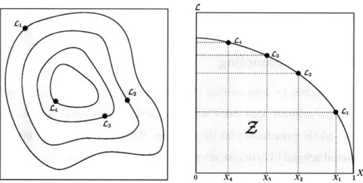
The procedure for determining each term in (3.15), shown graphically in Figure 3-1 and discussed in [16, 5], begins with drawing N 'live' points randomly from the entire prior distribution, corresponding to an initial value of Xo = 1 for the remaining prior mass. The lowest of the N likelihood values becomes Lo, and its corresponding

lX

Figure 3-1: A simple graphical representation of four iterations of the nested sampling algorithm. In the left-hand image, samples with successively larger likelihoods Li, weighted by their corresponding prior mass Xi = exp(-i/N) (or a trapezoidal weight wi as defined in (3.15)) add to the evidence integral in the right-hand image. Live

points are not shown. Borrowed from [5].

point is replaced by another drawn from the prior distribution, subject to the hard constraint L > Lo. The prior mass is then reduced by a factor exp(-1/N), so that the new prior mass is X1 = exp(-1/N), and the lowest likelihood value of the new

set of N live points is selected as L1. The process of replacing the ith least likely point

by one constrained to L > Li and setting the next prior mass Xi = exp(-i/N) is

repeated until the Mth iteration, in which the largest value of AZM = LmaxXM from

the pool of N live points that could contribute to the evidence is smaller than some user-defined tolerance.

The value for Xi can be derived as follows [16]. Let Xi = tiXi_1, where ti is drawn

from the distribution P(t) = NtN -_{l, i.e. the largest of N samples from U(O, 1). This}

is effectively what occurs in the selection of the least likely live point, since the lowest likelihood corresponds to the largest area. Working in logarithmic values, the mean and standard deviation of the dominant term log t are

1 1

< logt >= N and alogt = N. (3.16)

Since each log ti is independently chosen, we have log Xi ; (-i-Vi)/N, and therefore

I I

we let Xi = exp(-i/N).

The major advantage of nested sampling is that one run through the above al-gorithm provides all the data necessary for determining the standard error in the evidence as well as the posterior sample. The uncertainty in the evidence is mostly due to the error in assigning each Xi _{to its mean value exp(-i/N) [16]. Initially,}

the likelihoods Li increase faster than the prior masses Xi decrease, so the evidence increments Liwi also increase. After a certain number of steps, the increase in Li

becomes slower than the decrease in Xi, so the Liwi values begin to decrease. The maximum value of Xi occurs at a e-H, where

H = P(X) log P(X)dX log (3.17)

is called the information or negative entropy. Thus, most of the evidence should be accumulated after NH AvrH steps, and the corresponding error in log -± Xi =

(-i + x/i)/N is

±/

Since the accumulation of errors in log Xi shifts the maximum value of Liw₂ away

from i n H by

±NV,

run through the algorithm, an accurate value for the log evidence is obtained:

log Z = log L w) VN. (3.18)

The nested sampling algorithm also provides the posterior samples, ordered by increasing likelihood, simply as the M points discarded in each repetition. Each point then has weight

Liwi

Pi = z (3.19)

The set of posterior samples can be used to determine marginalized posterior distri-butions and to calculate means and standard deviations for each of the parameters in the model R-. Since the distribution of live points is increasingly more constrained with each iteration, the maximum likelihood estimate for the model parameters can be taken as the point in the Mth set of live points with the highest likelihood (i.e.

(3-

•---. ,,1 _ .

Figure 3-2: Ellipsoidal nested sampling with a bimodal distribution in two dimensions. As the ellipsoid (shown in red) is tightened with each iteration, the acceptance rate reduces because the regions of high likelihood are clustered at the two ends of the ellipsoid. Sampling from the two clusters individually will give a higher acceptance rate and requires fewer likelihood evaluations. Borrowed from [5].

the point corresponding to the likelihood Lmnx that satisfies the stopping criterion). Multimodal Nested Sampling

The implementation of the nested sampling algorithm used for this analysis [5] is based on an ellipsoidal nested sampling method developed by Mukherjee et al. [12] and modified by Shaw et al. [15]. Mukherjee et al. [12] introduce the method of approximating each likelihood surface as a multidimensional ellipsoid enclosing the current set of live points. The ellipsoid is enlarged by a factor f to account for the differences between the likelihood surface and the ellipsoid. New points at the it_h iteration are then sampled from the prior within the ellipsoid. This method runs into problems when the posterior distribution has multiple modes. Figure 3-2 shows a simple bimodal distribution with several iterations of ellipsoidal sampling. In the second-to-last panel, the regions of high likelihood are clustered at either end of the ellipsoid, so the acceptance rate for sampling new live points is reduced, and more likelihood evaluations are necessary to correctly sample the entire distribution.

Shaw et al. [15] extend this method to multimodal distributions by using a k-means algorithm with k = 2 (see e.g. [11]) to recursively partition the live points into separate clusters, as long as (i) the total volume of the new ellipsoids is less than a fraction of their parent ellipsoid and (ii) the new clusters are not overlapping. The final panel in Figure 3-2 shows the two modes and their individual ellipsoids.

Feroz et al. [5] build on the sampling method above by inferring the number of necessary clusters at each iteration instead of fixing k = 2. This is done using the

x-means algorithm [14], which determines the number of clusters by maximizing the Bayesian Information Criterion (BIC),

k

BIC(Mk) = log Lk - - log D (3.20) 2

where Mk is the model for the data having k clusters, Lk is the likelihood of that model at the maximum likelihood point, and D is the dimensionality of the problem. Notice that the BIC incorporates a penalty for more clusters and more dimensions to the problem. This method occasionally returns the incorrect number of clusters, but other methods for clustering are more computationally intensive, thus x-means is the method applied for this implementation. Also, the main purpose of this clus-tering method is to increase the efficiency of the algorithm by reducing the amount of unnecessary parameter space that is sampled at each iteration, so any mistakes in clustering should not affect the accuracy of the results.

The authors also use a dynamic enlargement factor fi,k for each iteration i and cluster k that takes into account the fraction of live points in each cluster, the prior volume Xi at each iteration, and the rate at which the enlargement factor itself changes. A cluster with more points will be more accurately sampled, thus requiring a smaller enlargement factor. A cluster with a smaller prior mass will also require less enlargement of its ellipsoid, since the prior mass tends to an ellipsoidal shape as it is constrained at each iteration.

Finally, the requirement for non-overlapping ellipsoids presented in [15] is relaxed. At each iteration, once K ellipsoids each with volume Vk are found, one is chosen randomly with probability

K

Pk = Vk/Vtot, where Vto t = Vk (3.21)

k=1

and a sample point subject to the current likelihood constraint is drawn from that ellipsoid. If the point lies within ne ellipsoids simultaneously, then the sample is accepted with a probability 1/ne.

Figure 3-3: A curving degeneracy that has been sub-clustered to improve efficiency. Borrowed from [5].

A unique application of such overlapping ellipsoids is a 'sub-clustering' method for working with pronounced degeneracies in the model. Figure 3-3 shows a curving degeneracy covered with eight subclusters. By dividing the ellipsoid at each iteration into several smaller overlapping clusters enclosed within it, the sampling efficiency is increased since at each iteration the ellipsoids have most of their area inside the regions of higher likelihood. The sub-clustering is performed using a k-means algorithm with

k = 2, and the resulting ellipsoids are additionally expanded relative to their neighbors to enclose the whole of the prior mass at each iteration.

Chapter 4

Preliminary Exploration of Nested

Sampling Approach

Before the nested sampling algorithm can be applied to reconstruction of real data, it requires testing on simulations of varying complexity. This chapter focuses on applying the nested sampling algorithm to a single pixel, generated using currently popular foreground models, and reconstructed using various subsets of these same models. We expect this analysis to be more accurate than an analysis of real data because the foregrounds have been greatly simplified; however, such an analysis will provide useful information about the behavior of the nested sampling algorithm that will aid in developing a method for testing the algorithm on real data.

This chapter begins by describing the data simulation, based on data that will be collected by the Planck Surveyor satellite, an upcoming all-sky survey with better sensitivity and frequency coverage than WMAP. We then discuss the accuracy of the nested sampling reconstruction of the data using a variety of models. Finally, we attempt to reconstruct a small patch of simulated data to get a glimpse at the accuracy of the nested sampling algorithm on a larger scale.

LFI HFI

v [GHz] 30 44 70 100 143 217 353 545 857

ao [AK] 19.25 19.25 18.08 8.17 4.67 6.42 2.66 2.05 0.68 Table 4.1: Each of the nine proposed frequency bands for the Planck Surveyor low and high frequency instruments (LFI and HFI), along with the RMS noise per 12' pixel. The first six noise widths were obtained from [4] and scaled to the correct pixel size. The last three noise widths were obtained from [10], converted to antenna temperature, then scaled to the correct pixel size.

4.1

Data Simulation

The data that we simulate is meant to imitate the data that will be collected by the Planck Surveyor satellite, scheduled for launch in December 2008. The Planck

Surveyor has two main components: the Low Frequency Instrument (LFI) that detects

the CMB signal in three lower frequency channels, and the High Frequency Instrument (HFI) that detects the signal in six higher frequency channels [10]. All nine channels are listed in Table 4.1, along with the RMS noise per 12' pixel for each frequency.

Figure 4-1 shows a simulated patch of sky for each of the four radiation components considered, in units of antenna temperature at a reference frequency of vo = 300GHz. This template was generated using the method discussed in [10] and converted from units of intensity to antenna temperature as discussed in Section 2.1. The images are composed of 400 x 400 pixels of width 1.5', spanning 10 x 10 deg2. The amplitudes in these maps are used as the amplitudes A, for each component c. The synchrotron, free-free and dust components are modeled using equations (2.4-2.7) with amplitudes

A, in antenna temperature, and the microwave background is modeled by equation

(2.2).

Before the data can be generated, we convolve the template in Figure 4-1 with a 30' FWHM Gaussian beam. We generate a discretized Gaussian beam matrix centered at the middle pixel of the image (ci, cy), with elements

a [(i-c2 )2

+ (j

Bij= exp - (i - )2 (j _ )2 (4.1) where a = aB/ap is the ratio of the beam width aB = 30'/2 log2 and the pixel

Thermal Dust Comoonent -4 -2 0 2 4 x (degrees) Free-Free Comoonent x (degrees) 0 x (degrees) Synchrotron Comnonent x (degrees)

Figure 4-1: 10 x 10 deg2 maps of the four radiation components at 300 GHz: (across horizontally from top left) CMB radiation, thermal dust emission, free-free emission and synchrotron emission. Each map contains 400 x 400 pixels, and each pixel is 1.5 arcmin wide. The data for these maps were taken from an image generated using a method discussed in [10], then converted to units of antenna temperature in pK.

dT/T

CMB Component

rr

>•

ri/T "A " COW"

I

z

'roI 143 Oaf CAWA CdA

td! X (qrft

I

[.

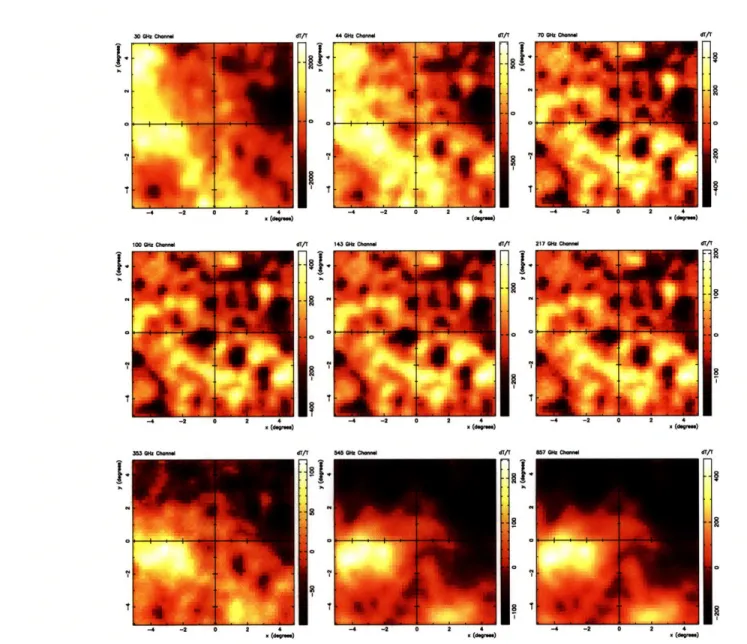
Figure 4-2: The summed components at each of nine frequency bands in Table 4.1, with the appropriate level of Gaussian noise. These 50 x 50 pixel maps were generated from the component maps in Figure 4-1, convolved with a 30' FWHM beam and downgraded to 12' pixels, as discussed in Section 4.1. The units of the data are antenna temperature in pK. __ -I/-100 QW Ch... "/T am CM ft- Ms7 Gbar Ch-· r, I

t

width a, = 1.5', and a = Eij Bij is the beam area. We then use a fast Fourier transform algorithm to transform both the beam Bij -* Bij and the four amplitude maps A, -- A, in order to perform the convolution as a multiplication in Fourier

space:

A/c = A -Bjj (4.2)

The convolved amplitudes are inverted back to position space, A -- Au. We then

downgrade the smoothed images to 12' pixels (i.e. 50 x 50 pixel images), using a bilinear interpolation method, in order to reduce the amount of noise on the data, since noise scales inversely with pixel size. The new amplitudes A ,, (where the primed pixel coordinates reflect the new pixel size) are then used to generate simulated data for each pixel.

For a single pixel at coordinates (i', j'), the nine data points for each frequency

Djv, , are calculated as a sum over the four components, plus Gaussian-distributed

random noise with zero mean and variance or, as listed in Table 4.1:

Ncomp

Di , = sc(v, i'jy') + n(O, ov). (4.3)

c=1

The input parameters Oij, are the three spectral indices 3

d = 4.67, Pf = -2.14 and

/8 = -2.7 and the four amplitudes Ai,, from the convolved and downgraded images

corresponding to the pixel. The energy spectra used for the components are (2.2) for the CMB component and (2.4-2.7) for the foregrounds. Figure 4-2 shows the summed components with noise at each of the nine frequencies in Table 4.1, as generated using this method.

4.2

Single Pixel Reconstruction

The likelihood function for a single pixel that is called by the nested sampling algo-rithm is

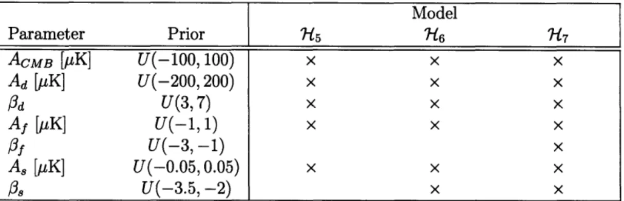
Model Parameter Prior 7-5 76 ₇ ACMB [pK] U(-100, 100) x x x Ad [M1K] U(-200, 200) x x x Pd U(3, 7) x x x Af [pK] U(-1, 1) x x x

Of

U(-3,-1)

x

Table 4.2: The seven component parameters and their corresponding prior distribu-tions. The models in which each parameter is allowed to vary are marked with an X.

where S(v, 8) = ZE-mP Sc(V, 8) is trial data calculated for sample parameters O.

The prior distribution for each parameter listed in Table 4.2 is selected as a uniform distribution with reasonable bounds.

The posterior distribution for the parameters is then sampled using the nested sampling algorithm with N = 300 live points and a tolerance AZmM < 0.05, as dis-cussed in Section 3.3.1, with three different proposed models for the data. The first model, which we will call R7-5, is one in which both the free-free and synchrotron spectral indices are fixed at their input values of = -2.14 and 0, = -2.7 for all the pixels, while the remaining five parameters are allowed to vary. This model simulates the case when the synchrotron and free-free spectral indices are known for the patch of sky in question. Since this is the case for our data, 7-R5 should produce results closest to the input data.

The second model 7R6 is the same as 15 but also allows P, to vary. The third model 717 allows all seven parameters to vary. Models 7-:6 and 7"17 simulate the case when less is known about the energy spectrum of the foregrounds, thus we test these to see how well the sampling algorithm is able to determine each of the parameters. Table 4.2 shows each of the three proposed models with their corresponding free parameters.

In the following sections, we discuss the results produced by the nested sampling algorithm for an individual pixel in Figure 4-2. We also apply the sampling algorithm

S

C

0

0 200 400 600 800 1000

Frequency (GHz)

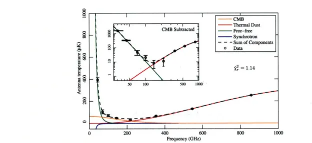
Figure 4-3: Energy spectrum for each CMB signal component (colored lines) and their sum S(v, 9) (dashed line), calculated at the maximum likelihood values

E

E,

with model -/ to a set of data generated using equation (2.3) for the dust component, in order to compare the evidence values for the two results. Finally, we apply the sampling algorithm using model 7-s5 to all the pixels in the sky patch.

4.2.1

Posterior Distributions

Figure 4-3 shows the energy spectrum of each component for a single pixel, as deter-mined by the maximum likelihood parameters

E

S(v, 8) (dashed line in the figure), the function which maximizes the likelihood (4.4).

The reduced X2 _{(for four effective degrees of freedom) for these parameters is 1.14, so}

they are a good fit to the data. We choose the maximum likelihood estimates for the parameters instead of following [4] and using the mean values of the posterior dis-tribution. This is because the nested sampling algorithm produces consistent results every time, and the prior region from which the maximum likelihood point is chosen is very small. Thus, the maximum likelihood point does not vary enough between runs to significantly affect the X2 .

calculated from 11 frequency bands, as well as data simulated using model (2.3) for the dust component. However, we use smaller pixels (thus more noisy data) and the same model for simulation and reconstruction of the data. Thus, the lower X2 _that

we obtain for this particular pixel is reasonable given our relative freedom over the parameter space and the similarity between the simulated data and proposed model. Also, the method used in [4] involves a combination of low- and high-resolution data, as well as a combination of analytical and MCMC methods in order to more accurately estimate the parameters, whereas our method produced reasonable estimates for all parameters simultaneously, using one sampling method and data with a relatively high resolution.

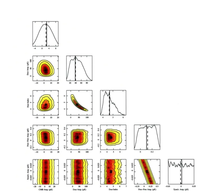
Figure 4-4 shows the posterior distribution for a single pixel produced by the nested sampling algorithm for model 745, marginalized into all the possible 1- and 2- dimensional distributions. This figure also shows the input parameters 0 (solid lines/square markers) and the maximum likelihood estimates G (dashed lines/triangle markers) for reference.

One noticeable feature of this distribution is that the sampling algorithm seems unable to find a peak in the marginal distribution for the amplitude of the synchrotron component. This can be explained by the fact that the input value and prior range for As were very small to begin with, thus changes in the parameter did not affect the likelihood very much. This is further evidenced by the fact that the reduced

X2 is low, despite the negative maximum likelihood estimate for A,, whereas the input value is positive. Also, the degeneracy between the free-free and synchrotron components, clearly visible in the joint probability distribution P(Af, A,), allows the two components to "compensate" for each other, so the negative synchrotron component is balanced by a slightly larger free-free amplitude.

Another interesting feature of the posterior distribution is the correctly sampled degeneracy between the dust component amplitude and index. The joint probability distribution P(Ad, Pd) displays a pronounced curving degeneracy, whose maximum likelihood point agrees well with the input value. This is a good representation of the algorithm's effectiveness with a sample size of - 8, 500 points, several orders of

-4 0 4 8 -10 0 10 20 20 40 60 80 -10 0 10 20 0 50 100 4 5 6 -10 0 10 20 0 50 100 3 4 5 6 0 0.2

slI

'%L1

TE:

3EL

~HL11~~

CMB Amp. (OK) Dust Amp. (jK) Dust Index Fre-Free Amp. (K) Synch. Amp. (gK)

Figure 4-4: The posterior distribution for model 7-s determined by the nested sam-pling algorithm, marginalized into all possible 1- and 2- dimensional distributions. The 1D distributions P(0i) for the five free parameters Oi are displayed along the di-agonal. The 2D distributions P(9i, 9j), where i = j, are displayed below the diagonal. The contours mark the la (68%), 2a (95%) and 3a (99.7%) confidence levels. The solid vertical lines in the 1D distributions and the square markers in the 2D distribu-tions denote the input parameters 8, while the dashed lines (ID) and triangles (2D) denote the maximum likelihood parameters 6 determined by the sampling algorithm.

0 -X $, 9 9 61 0

magnitude less than the number of samples necessary for an accurate MCMC sampled posterior distribution.

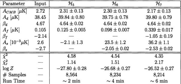
Figures 4-5 and 4-6 show the posterior distributions for models 7I₆ and R77.

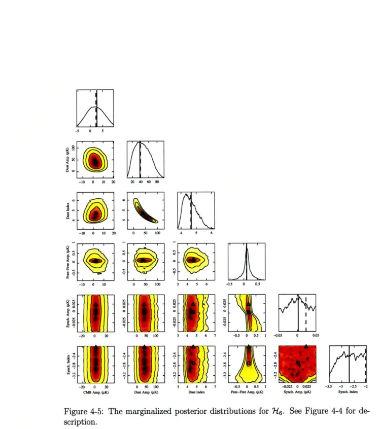
The CMB amplitude, dust amplitude and dust spectral index are relatively well-determined and their distributions show good consistency between the three models. However, the degeneracy between the synchrotron and free-free component parame-ters causes problems for the sampling algorithm. Although the free-free amplitude is well-determined with model W6, the free synchrotron spectral index seems to in-troduce too much freedom and prevents the sampling algorithm from determining a clear peak in the posterior distribution. This problem is amplified in the posterior distribution for 7t, which does not exhibit clear constrains for any of the four free-free or synchrotron radiation components, although it does restrict the parameter space of both A8 and Af so that at least one must be positive.

A final striking difference between our posterior distributions and those of [4] is that their posterior distributions appear to lack any of the massive degeneracies that appear in our data, and all their marginal distributions have well-behaved contours. This could mean that we should model the foreground components some other way in order for the nested sampling algorithm to be able to constrain the parameters. For example, Eriksen et al. [4] suggest combining both free-free and synchrotron radiation components into one effective foreground.

4.2.2

Model Comparison

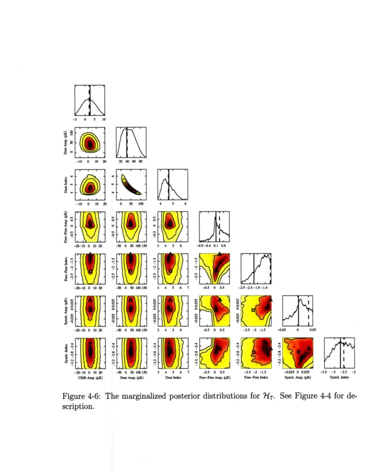
The maximum likelihood estimates and standard errors for each of the three pro-posed models are shown in Table 4.3, along with the evidence and X2 values for each model. As discussed in the previous section, the parameters ACMB, Ad and Pd are well-determined with each of the three models, and this is supported by the similar maximum likelihood estimates between the models. However, the estimates for the free-free and synchrotron components vary from the input values by factors of two or even ten. The increasing trend in the reduced ^2 is evidence of the problem with these two foreground components. Nevertheless, the increasing evidence and

decreas-Parameter Input

["15

Run Time - 2 min - 4 min - 6 min

Table 4.3: Maximum likelihood estimates and standard errors for the free parameters in each of three proposed models for the data, along with the evidence (log Z) with standard error, total

k2,

k

model. Run times are for a Sun Fire V480 machine from the MRAO Sun cluster with 16G RAM and a clock speed of 150 MHz.

ing total X2 point to the fact that the models with more free parameters are better able to describe the data.

The Bayesian evidence Z that the nested sampling algorithm produces allows us to choose which model best describes the data. Comparing the three evidence values,

R1-5 seems to be disfavored by a factor of A log Z - 1 with respect to both R7"6 and 717.

According to [15], this is on the border between a 'significant' and 'not significant' difference between evidence values, thus in this situation the result is inconclusive. It appears that all three models are equally fitting, which is reasonable given that the underlying equations for both simulation and reconstruction were the same. Although inspection of the parameter estimates indicates that 75 should be the best model for the given data since most of its parameter estimates are near the input values, the spread of high likelihood regions in the higher-dimensional models makes it difficult to rule them out as possibilities. Thus, more work needs to be done in order to be able to clearly distinguish between models in such a problem.

Another indication of modeling difficulties is the following experiment. We simu-lated a new set of data D,,'j using the two-component dust model (2.3) as in [4], then

-5 0 5 -10 0 10 20 20 40 60 80 ji I -10 0 10 20 0 50 100 4 5 6 -10 0 10 0 50 100 3 4 5 6 -0.5 0 0.5 -20 0 20 0 50 100 3 4 5 6 7 -0.5 0 0.5 1 -0.05 0 0.05

:0

:0

CMB Amp. (IK) Dust Amp. (;K) Dust Index Free-Free Amp. (gK) Synch. Amp. (K) Synch. Index

Figure 4-5: The marginalized posterior distributions for R76. See Figure 4-4 for

de-scription. W• 9" a 9 9 N 0 ci_I N *i_i t N OD Fi N d oo rj Fl n

-5 0 5 10 -10 0 10 20

Ec&,

Dust Amp. (iK)

4 5 6 3 4 5 6 3 4 5 6 7 3 4 5 6 3 4 5 6 7 Dust Index -0.9 -0.4 0.1 0.6 7_{-0.5 0 0.5} -0.5 0 0.5 -2.9 -2.4 -1.9 -1.4 -2.5 -2 -1.5 -. 05 0 0.05

Kl

NL

Free-Free Amp. (ILK)

-2.5 -2 -1.5 Free-Free Index

-0.025 0 0.025 Synch. Amp. (iLK)

-3.5 -3 -2.5 -2 Synch. Index

Figure 4-6: The marginalized posterior distributions for Rl7. See Figure 4-4 for

de-scription. 9 I r! 9 N_I r F:_I F; c I

Parameters Input ?H5 with D' ACMB [pK] 2.72 2.32 ± 0.13 Ad [/tK] 38.45 39.95 + 0.86

Pd

Table 4.4: Maximum likelihood estimates of the parameters in model 7H5 applied to the data D' generated using the two-component dust model, as discussed in the text. The j2 and log Z values indicate that 715 may be a better fit to D' than to D. modeled these data using 75 as before. Table 4.4 shows the maximum likelihood parameters, evidence and X2 values for these results. The parameter estimates are similar to those in Table 4.3 for 75, with the only difference appearing in

Pd

?15 on both datasets D and D' should give us an indication of which set of data best fits the model. Surprisingly, the X2 and log Z values indicate that 15 is able to fit D'

slightly better than D, although as stated earlier, the difference between the evidence values is not significant enough to be conclusive.

4.3

Full Map Reconstruction

The results discussed in the previous section were collected on a Sun Fire V480 machine with 16G RAM and a clock speed of 150 MHz. As shown in Table 4.3, the run time to generate one posterior sample for each model increases linearly with the number of free parameters. Although the run times are a bit long for a single pixel on this machine, running the sampling algorithm on a supercomputer such as COSMOS (whose 152 Itanium2 processors each have a clock speed of 1.3 GHz [2]) would produce results in a tenth of a second for a single pixel, thus reconstructing the entire sky patch at full resolution (400 x 400 pixels) would take about four hours with 7?5.