6000 Broken Sound Parkway, NW Suite 300, Boca Raton, FL 33487 711 Third Avenue
New York, NY 10017 2 Park Square, Milton Park Abingdon, Oxon OX14 4RN, UK an informa business
www.taylorandfrancisgroup.com
K20728
MatheMatical techniques in GIS Dale
Ma the M a tic al techniques in GIS
SECOND EDITION
“The insight provided by this book is extremely valuable. It represents a significant effort to explain—in an interesting and pedagogical way—the basic mathematical techniques and principles underpinning the manipulation of geographical data. Modern technologies have made the “where” highly important, and computers and mobile devices provide all kinds of sophisticated solutions to deal with this issue. However, it is worth remember- ing that eventually only good data and good processing will provide reliable information.
The mathematics behind this processing thereby becomes essential. This book enables an easy access to the rules and manipulations applied behind the scene. This book is needed.”
––Stig Enemark, Professor of Land Management, Department of Development and Planning, Aalborg University, Denmark
“… an excellent introduction to the mathematics behind these complexities. By having some understanding of the technology behind GIS, users are better able to ensure the data and results from GIS are “fit for purpose” and can be safely used. … I enthusiastically encourage GIS users to read this book.”
—Ian P. Williamson, Emeritus Professor, The University of Melbourne
“Professor Peter Dale is one of the great pioneers of the GIS and geomatics fields, hav- ing made seminal contributions to the development and application of the technology in support of natural resource management and land administration. His writing is richly informed by both a deep intellect and a wealth of experience.”
—John McLaughlin, President Emeritus, University of New Brunswick
See What’s New in the Second Edition:
• Summaries at the end of each chapter
• Worked examples of techniques described
• Additional material on matrices and vectors
• Further material on map projections
• New material on spatial correlation
• A new section on global positioning systems
Peter Dale
S E C O N D E D I T I O N
CAT#K20728 cover.indd 1 4/9/14 9:22 AM
MatheMatical techniques
in GIS
S E C O N D E D I T I O N
Boca Raton London New York CRC Press is an imprint of the
Taylor & Francis Group, an informa business
Peter Dale
MatheMatical techniques
in GIS
S E C O N D E D I T I O N
Boca Raton, FL 33487-2742
© 2004 by Taylor & Francis Group, LLC
CRC Press is an imprint of Taylor & Francis Group, an Informa business No claim to original U.S. Government works
Version Date: 20140306
International Standard Book Number-13: 978-1-4665-9555-2 (eBook - PDF)
This book contains information obtained from authentic and highly regarded sources. Reasonable efforts have been made to publish reliable data and information, but the author and publisher cannot assume responsibility for the validity of all materials or the consequences of their use. The authors and publishers have attempted to trace the copyright holders of all material reproduced in this publication and apologize to copyright holders if permission to publish in this form has not been obtained. If any copyright material has not been acknowledged please write and let us know so we may rectify in any future reprint.
Except as permitted under U.S. Copyright Law, no part of this book may be reprinted, reproduced, transmit- ted, or utilized in any form by any electronic, mechanical, or other means, now known or hereafter invented, including photocopying, microfilming, and recording, or in any information storage or retrieval system, without written permission from the publishers.
For permission to photocopy or use material electronically from this work, please access www.copyright.
com (http://www.copyright.com/) or contact the Copyright Clearance Center, Inc. (CCC), 222 Rosewood Drive, Danvers, MA 01923, 978-750-8400. CCC is a not-for-profit organization that provides licenses and registration for a variety of users. For organizations that have been granted a photocopy license by the CCC, a separate system of payment has been arranged.
Trademark Notice: Product or corporate names may be trademarks or registered trademarks, and are used only for identification and explanation without intent to infringe.
Visit the Taylor & Francis Web site at http://www.taylorandfrancis.com and the CRC Press Web site at http://www.crcpress.com
v
Contents
Preface to Second Edition ...ix
Preface to First Edition ...xi
The Author ... xiii
List of Tables ...xv
List of Illustrations ...xvii
List of Boxes ... xxiii
List of Examples ...xxv
Chapter 1 Characteristics of Geographic Information...1
1.1 Geographic Information and Data ...1
1.2 Categories of Data ...2
Summary ... 10
Chapter 2 Numbers and Numerical Analysis ... 13
2.1 The Rules of Arithmetic ... 13
2.2 The Binary System ... 18
2.3 Square Roots ...20
2.4 Indices and Logarithms ...22
Summary ...29
Chapter 3 Algebra: Treating Numbers as Symbols ... 33
3.1 The Theorem of Pythagoras ... 33
3.2 The Equations for Intersecting Lines ... 35
3.3 Points in Polygons... 41
3.4 The Equation for a Plane ... 43
3.5 Further Algebraic Equations ... 43
3.6 Functions and Graphs ... 49
3.7 Interpolating Intermediate Values ... 52
Summary ... 55
Chapter 4 The Geometry of Common Shapes ... 59
4.1 Triangles and Circles ... 59
4.2 Areas of Triangles ... 62
4.3 Centers of a Triangle ...66
4.4 Polygons ...69
4.5 The Sphere and the Ellipse ... 71
4.6 Sections of a Cone ... 73
Summary ... 78
Chapter 5 Plane and Spherical Trigonometry ... 81
5.1 Basic Trigonometric Functions ... 81
5.2 Obtuse Angles ...85
5.3 Combined Angles ...89
5.4 Bearings and Distances ... 91
5.5 Angles on a Sphere ... 95
Summary ... 100
Chapter 6 Differential and Integral Calculus ... 103
6.1 Differentiation ... 103
6.2 Differentiating Trigonometric Functions ... 108
6.3 Polynomial Functions ... 111
6.4 Linearization ... 114
6.5 Basic Integration ... 118
6.6 Areas and Volumes ... 120
Summary ... 125
Chapter 7 Matrices and Determinants ... 129
7.1 Basic Matrix Operations ... 129
7.2 Determinants ... 134
7.3 Related Matrices ... 138
7.4 Applying Matrices ... 144
7.5 Rotations and Translations ... 146
7.6 Simplifying Matrices ... 155
Summary ... 161
Chapter 8 Vectors ... 163
8.1 The Nature of Vectors ... 163
8.2 Dot and Cross Products ... 167
8.3 Vectors and Planes ... 170
8.4 Angles of Incidence ... 173
8.5 Vectors and Rotations ... 174
Summary ... 178
Chapter 9 Curves and Surfaces ... 181
9.1 Parametric Forms ... 181
9.2 The Ellipse ... 186
9.3 The Radius of Curvature ... 189
9.4 Fitting Curves to Points ... 191
9.5 The Bezier Curve ... 198
9.6 B-Splines ...200
Summary ...202
Chapter 10 2D/3D Transformations ...205
10.1 Homogeneous Coordinates ...205
10.2 Rotating an Object ...207
10.3 Hidden Lines and Surfaces ... 216
10.4 Photogrammetric Measurements ... 218
Summary ... 221
Chapter 11 Map Projections ...223
11.1 Map Projections ...223
11.2 Cylindrical Projections ...226
11.3 Azimuthal Projections ... 231
11.4 Conical Projections ...234
Summary ... 241
Chapter 12 Basic Statistics ... 243
12.1 Probabilities ... 243
12.2 Measures of Central Tendency ...246
12.3 The Normal Distribution ... 252
12.4 Levels of Significance... 255
12.5 The t-Test ... 259
12.6 Analysis of Variance ...260
12.7 The Chi-Squared Test ...265
12.8 The Poisson Distribution ...266
Summary ...268
Chapter 13 Correlation and Regression ... 271
13.1 Correlation ... 271
13.2 Regression... 275
13.3 Weights ...280
13.4 Spatial Autocorrelation ...282
Summary ...286
Chapter 14 Best-Fit Solutions ...289
14.1 Least Square Solutions ...289
14.2 Survey Adjustments ... 295
14.3 Satellite Position Fixing ...307
Summary ... 315
Further Reading ... 317
ix
Preface to Second Edition
Many people wishing to make use of geographic information systems (GIS) start from a limited mathematical background. In Mathematical Techniques in GIS, Second Edition, the text as before focuses on those who are unfamiliar with mathe- matics and need to understand the principles behind the manipulation of spatial data.
The new text adds additional material. The first nine chapters lay out the basic foun- dations and introduce the reader to the relevant techniques and shorthand notations that frequently occur in mathematics; the remaining five chapters build on the earlier material. These later chapters place particular emphasis on the use of the techniques in GIS and geomatics. Throughout the text there are a number of examples shown in boxes and there is a summary at the end of each chapter listing all the important ideas that have been introduced.
xi
Preface to First Edition
This book has been written for nonmathematicians who wish to understand some of the assumptions that underlie the manipulation and display of geographic infor- mation. It assumes very little basic knowledge of mathematics but moves rapidly through a wide range of data transformations, outlining the techniques involved.
Many of these are precise, building logically from certain underlying assumptions;
others are based on statistical analysis and the pursuit of the optimum rather than the perfect and definite solution.
Mathematics has its own form of shorthand that often gets in the way of under- standing what is going on. For those who are unfamiliar with mathematical notation this can be daunting; but it cannot be avoided. It can in many cases be kept to a minimum and in what follows, the derivation of some of the formulae is placed in boxes that can be digested at leisure without interrupting the narrative. But at the end of the day, compromise has had to be made and as the text progresses there is an increasing use of symbols.
This spirit of compromise is most apparent in the selection of topics discussed.
Many things have had to be left out—indeed every chapter could be expanded to a full book and most would require several volumes in order to do their subject jus- tice. Introduction to Mathematical Techniques Used in GIS is therefore a book that allows the reader to get started and then to turn to the many more informative texts that are available.
The text begins with an introduction to geographic data but soon focuses on the
“where” rather than the “what.” It assumes that the data have been measured and refrains from discussing the techniques of measurement science, other than to rec- ognize that measurement is prone to error. Pure mathematics, even when dealing with vague concepts, provides precise answers that can be verified by anyone. Even statistical analysis uses processes that can be programmed into a computer to give a consistent answer, even when the underlying assumptions are not met or the hypoth- esis has been incorrectly formulated. The apparent exactness of an answer does not mean that it is correct. To understand the output from, for example, a geographic information system, one needs to understand the quality of the data that are entered into the system, the algorithms behind the data processing, and the limitations of the graphic displays.
This book deals with only part of the bigger picture. It focuses on the basic math- ematical techniques, building the whole of mathematics in a series of steps that are the foundations for a deeper understanding. It seeks to lay the foundations for the more complex forms of manipulation that arise in the handling of spatially related data.
The technology behind geographic information systems (GIS) allows such data to be gathered, processed, and displayed. The power and appeal of such systems often lie in their graphical output, the maps that they create. Users of GIS need to understand the quality of that output so that they can advise others on the integrity of
their results. The issue is not a matter of which buttons to push but rather of the qual- ity of the information that has been produced. Quality means “fitness for purpose”
and “safety in use.”
This book therefore looks at some of the fundamentals and provides an introduc- tion to spatial data manipulation through which users of GIS may come to under- stand whether what they do results in what can genuinely be described as a “quality product.” It has been copy edited for an American market, hence the spelling of words such as “meter” for the English “metre” and “center” for “centre.”
xiii
The Author
Peter Dale trained as a land surveyor and worked for seven years in Uganda before entering the academic world. He ultimately became a professor in land information management at the University College London. He is an Honorary President of the International Federation of Surveyors and was awarded an OBE in recognition of his services to surveying. He is now retired and lives in a remote area of Scotland. Peter Dale can be contacted via e-mail at: [email protected].
xv
List of Tables
TABLE 1.1 Points, Lines, and Areas on Maps ...3
TABLE 1.2 The Greek Alphabet ...6
TABLE 2.1 Standard Symbols ... 14
TABLE 2.2 Example of Seven-Figure Common Logarithms ...24
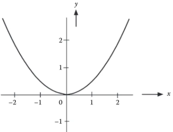
TABLE 3.1 Values of y and x for y = 0.5x2 ... 51
TABLE 5.1 Signs of Sine, Cosine, and Tangent ...88
TABLE 6.1 Data for y = 1 + 9x – 6x2+ x3 ... 107
TABLE 12.1 Partial Areas under the Normal Curve ... 255
TABLE 12.2 Levels of Significance (p) for Values of t (Given 9 Degrees of Freedom) ...260
TABLE 12.3 Data Classified into Rows and Columns ... 262
TABLE 13.1 Framework for Calculating r ... 273
TABLE 14.1 Conditions to Be Satisfied: MX + L = 0 ...290
TABLE 14.2 The Normal Equations: MT(MX + L) = 0 ... 291
TABLE 14.3 Weighted Normal Equations: MTWMX + MTWL = 0 ...293
TABLE 14.4 Observations and Conditions: M(O + ε) + L = 0 ...296
TABLE 14.5 The Relationships to Be Optimized: Mε + R = 0 ...296
TABLE 14.6 The Differential Equations: M(δε) = 0 ...297
TABLE 14.7 The Relationships between the Correlatives: MTK = Wε ... 297
TABLE 14.8 The Equations for the Correlatives ... 298
TABLE 14.9 Solving for the Correlatives ... 298
xvii
List of Illustrations
FIGURE 1.1 A scale bar. ...3
FIGURE 1.2 Rectangular Cartesian coordinates. ...4
FIGURE 1.3 Nonrectangular or skewed grid. ...4
FIGURE 1.4 Polar coordinates. ...5
FIGURE 1.5 Latitude and longitude. ...6
FIGURE 1.6 Straight-line distances. ...7
FIGURE 1.7 Lines as vectors. ...7
FIGURE 1.8 A line as a raster image. ...8
FIGURE 1.9 Topology. ...9
FIGURE 1.10 Union and intersection of data sets A and B. ...9
FIGURE 2.1 Rotating a dice (forward + sideways or sideways + forward). ... 15
FIGURE 2.2 The distance from A to B. ... 21
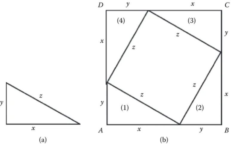
FIGURE 3.1 Rotating a triangle to prove Pythagoras’s theorem. ...34
FIGURE 3.2 Intersecting lines. ... 35
FIGURE 3.3 The slope of a line. ...36
FIGURE 3.4 Parallel lines. ... 39
FIGURE 3.5 Distance offset from a line. ... 39
FIGURE 3.6 Clipping to a window. ...40
FIGURE 3.7 Similar triangles. ... 41
FIGURE 3.8 Point-in-polygon. ... 42
FIGURE 3.9 A plane surface. ... 45
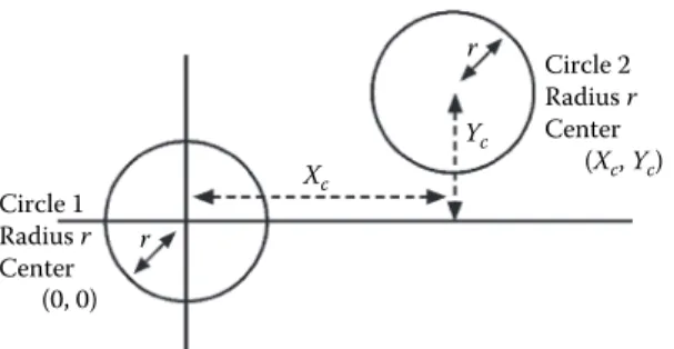
FIGURE 3.10 The equation of a circle. ...46
FIGURE 3.11 Graph of the function y = 0.5x2. ... 51
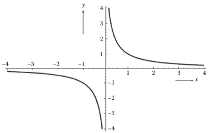
FIGURE 3.12 Graph of y = 1/x. ... 52
FIGURE 3.13 Linear interpolation and extrapolation. ... 52
FIGURE 3.14 The midpoints of the sides of a triangle. ... 53
FIGURE 3.15 Interpolation of heights down a slope. ...54
FIGURE 3.16 Interpolating contours between spot heights. ...54
FIGURE 3.17 Alternative triangulation networks. ... 55
FIGURE 4.1 The angles of a triangle. ...60
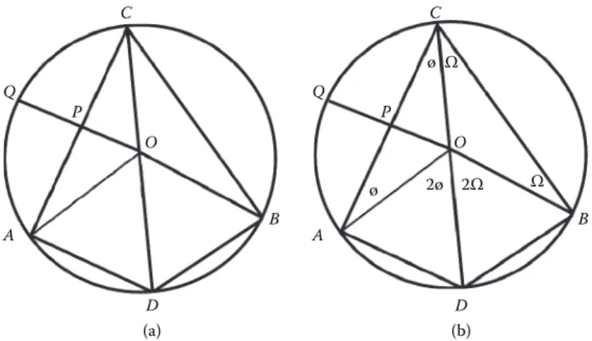
FIGURE 4.2 Angles subtended by arcs. ... 61
FIGURE 4.3 The area of a triangle. ... 62
FIGURE 4.4 The area of a trapezium. ...64
FIGURE 4.5 The area of a triangle by coordinates. ...65
FIGURE 4.6 The centroid. ...66
FIGURE 4.7 The orthocenter. ... 67
FIGURE 4.8 The incenter. ... 67
FIGURE 4.9 The circumcenter. ...68
FIGURE 4.10 Inscribed and circumscribed circles. ...68
FIGURE 4.11 Straight-line figures. ...69
FIGURE 4.12 Two ways to divide a quadrilateral. ... 69
FIGURE 4.13 Triangulation networks. ... 70
FIGURE 4.14 Thiessen polygons and the Delaunay triangles. ... 71
FIGURE 4.15 Great and small circles. ... 72
FIGURE 4.16 Ellipse and auxiliary circle. ... 72
FIGURE 4.17 An ellipse and its directrix. ... 73
FIGURE 4.18 An enclosed ellipse. ... 75
FIGURE 4.19 A parabola. ... 75
FIGURE 4.20 A hyperbola with its asymptotes. ... 76
FIGURE 4.21 Two intersecting hyperbolae. ... 76
FIGURE 4.22 A double cone. ...77
FIGURE 4.23 Sections of a cone—circle and ellipse. ...77
FIGURE 4.24 Sections of a cone—parabola and hyperbola. ... 78
FIGURE 5.1 Similar right-angled triangles. ...82
FIGURE 5.2 The height or altitude of a triangle. ... 83
FIGURE 5.3 Toward a right angle. ...85
FIGURE 5.4 A circle with unit radius. ...86
FIGURE 5.5 Angles in the second quadrant. ...86
FIGURE 5.6 Angles in the third and fourth quadrants. ...87
FIGURE 5.7 The cycle of values of sin A. ... 88
FIGURE 5.8 Combining adjacent angles. ... 89
FIGURE 5.9 Angle and bearing measurements. ...92
FIGURE 5.10 Fixing points from observed angles. ...92
FIGURE 5.11 A traverse. ...94
FIGURE 5.12 The spherical triangle. ...96
FIGURE 5.13 Spherical angles. ...97
FIGURE 5.14 The sine formula for spherical triangles. ...97
FIGURE 5.15 The cosine formula for spherical triangles. ... 98
FIGURE 5.16 Colatitudes AN, BN. ...99
FIGURE 6.1 Tangents to a curve. ... 104
FIGURE 6.2 The slope and the normal to a curve. ... 104
FIGURE 6.3 (a) A cubic curve and (b) a quartic. ... 107
FIGURE 6.4 Small angles. ... 108
FIGURE 6.5 Area beneath a curve. ... 121
FIGURE 6.6 Area of an irregular shape. ... 123
FIGURE 6.7 An ellipse cut into four strips. ...124
FIGURE 6.8 Volumes of a cylinder and cone. ... 125
FIGURE 7.1 Submatrices and minors. ... 140
FIGURE 7.2 Shift or translation of origin. ... 146
FIGURE 7.3 Reflection in the y-axis. ... 147
FIGURE 7.4 Rotation of axes. ... 148
FIGURE 7.5 A skewed grid. ... 150
FIGURE 7.7 Left- and right-hand rules. ... 153
FIGURE 7.6 Rotating a rectangle. ... 153
FIGURE 7.8 Positive rotations around each axis—left-hand rule. ... 153
FIGURE 8.1 The axes i, j, k for vector P. ... 164
FIGURE 8.2 Vector addition. ... 164
FIGURE 8.3 Direction cosines. ... 165 FIGURE 8.4 Dot and cross products. ... 167 FIGURE 8.5 A parallelepiped. ... 169 FIGURE 8.6 Vectors and a plane. ... 171 FIGURE 8.7 Angle of incidence. ... 174 FIGURE 8.8 Rotation using vectors. ... 176 FIGURE 9.1 Orthogonal lines. ... 182 FIGURE 9.2 Tangents to a circle and an ellipse. ... 182 FIGURE 9.3 The ellipse and auxiliary circle. ... 183 FIGURE 9.4 Normal to an ellipse. ... 186 FIGURE 9.5 Theta and phi. ... 188 FIGURE 9.6 Radius of curvature. ... 190 FIGURE 9.7 Fitting a second-degree (quadratic) curve. ... 193 FIGURE 9.8 Two quadratics fitted to three points. ... 195 FIGURE 9.9 A piecewise cubic. ... 196 FIGURE 9.10 Looping curve. ... 197 FIGURE 9.11 A Bezier curve with two control points. ... 198 FIGURE 9.12 Two versions of a Bezier curve. ... 199 FIGURE 9.13 B-spline and knots. ... 201 FIGURE 10.1 Points at infinity. ...206 FIGURE 10.2 Vanishing points for a rectangular block. ...206 FIGURE 10.3 A barn. ...209 FIGURE 10.4 The barn after two rotations. ... 213 FIGURE 10.5 The affine and perspective projections of the barn. ... 214 FIGURE 10.6 Transformation into a perspective view. ... 215 FIGURE 10.7 Stereo pair of aerial photographs. ... 218 FIGURE 10.8 Principal point in the center of an aerial photograph. ... 219 FIGURE 10.9 Photogrammetric rotations. ... 219 FIGURE 10.10 Model area for overlapping stereo pair of photographs. ... 221 FIGURE 11.1 Points on a globe. ...224
FIGURE 11.2 The simple cylindrical projection. ...224 FIGURE 11.3 The elemental triangle on a sphere and on a plane surface. ...225 FIGURE 11.4 Cylinder, cone, and plane. ...225 FIGURE 11.5 Cylindrical equidistant (a), equal area (b), and conformal (c). ...226 FIGURE 11.6 The Transverse Mercator. ...228 FIGURE 11.7 Zenithal projection. ... 231 FIGURE 11.8 Oblique azimuthal. ... 232 FIGURE 11.9 Conical projection with one or two standard parallels. ... 235 FIGURE 11.10 Elemental triangles for conical projections. ... 235 FIGURE 11.11 Conical equidistant with one standard parallel. ... 236 FIGURE 11.12 A conical projection with two standard parallels. ... 239 FIGURE 12.1 Population and sample. ...244 FIGURE 12.2 A plot of equal probability after 15 events. ... 247 FIGURE 12.3 A plot of probability for n events. ...254 FIGURE 12.4 Percentage of distribution within one, two, and three
standard deviations from the mean. ...254 FIGURE 12.5 One- and two-tailed tests. ... 262 FIGURE 13.1 Correlation between X and Y. ... 272 FIGURE 13.2 Regression line. ... 276 FIGURE 13.3 Residuals from the regression line. ... 276 FIGURE 13.4 Example of a regression line. ... 277 FIGURE 13.5 Residuals from fitting a straight line to an elliptical curve. ...282 FIGURE 13.6 A set of polygons and the contiguity matrix. ...284 FIGURE 13.7 Contiguity cases. ...284 FIGURE 14.1 The braced quadrilateral. ...299 FIGURE 14.2 Four satellites and a receiver. ...307
xxiii
List of Boxes
BOX 2.1 Axioms of Arithmetic ... 14 BOX 2.2 Rules of Arithmetic ... 16 BOX 2.3 Further Rules of Arithmetic ... 23 BOX 2.4 Rules for Logarithms ...26 BOX 2.5 Logarithms to the Base 10 ...27 BOX 3.1 One Proof of Pythagoras’s Theorem ...34 BOX 3.2 The Intersection of Two Planes ...44 BOX 3.3 Interpolation—The Coordinates of the Centroid of a Triangle ... 53 BOX 4.1 Angles of a Triangle and in a Circle ...60 BOX 4.2 The Area of a Triangle from Its Semiperimeter ... 63 BOX 4.3 The Area of a Triangle and a Trapezium ...64 BOX 4.4 The Area of a Polygon ...66 BOX 4.5 Centers of a Triangle ...68 BOX 4.6 The Angles of a Polygon ... 69 BOX 5.1 Basic Relationships ...82 BOX 5.2 Sine and Cosine Formulae for Any Plane Triangle ...85 BOX 5.3 Combined Angles ...90 BOX 5.4 Trigonometrical Functions and the Semiperimeter ... 91 BOX 5.5 Coordinates from Observed Angles ...93 BOX 5.6 Sine and Cosine Formulae for Spherical Triangles ...99 BOX 6.1 Basic Differentials ... 105 BOX 6.2 Differentiating Trigonometrical Functions ... 111 BOX 6.3 Maclaurin’s Theorem ... 113 BOX 6.4 Taylor’s Theorem ... 116 BOX 6.5 Summary of Integrals ... 119 BOX 6.6 Combined Functions ... 120 BOX 6.7 Area of Irregular Shapes ... 123
BOX 7.1 Matrix Addition and Subtraction ... 131 BOX 7.2 Matrix Multiplication (1) ... 132 BOX 7.3 The Determinant of a Matrix ... 135 BOX 7.4 Matrix Multiplication (2) ... 139 BOX 7.5 Inverses and Transposes of Square Matrices ... 144 BOX 7.6 The Intersection of Two Lines ... 145 BOX 7.7 Rotation of Axes ... 151 BOX 8.1 Vector Multiplication ... 170 BOX 8.2 The Equation of a Plane ... 172 BOX 9.1 Parametric Equations for Lines and Conic Sections
(Second-Degree Curves) ... 185 BOX 9.2 The Radius ν ... 188 BOX 9.3 Radii of Curvature ... 191 BOX 11.1 Cylindrical Projections for a Sphere ... 230 BOX 11.2 Zenithal Projections ... 233 BOX 11.3 Conical Projections of the Sphere ... 238 BOX 11.4 Lambert’s Projection of the Ellipsoid ...240 BOX 12.1 The Binomial Expansion ...245 BOX 12.2 The Binomial Coefficients ...246 BOX 12.3 Variance and Standard Deviation ...248 BOX 12.4 Mean Outcome from Binomial Expansion ...250 BOX 12.5 The Binomial Distribution—Variance and Standard Deviation ... 251 BOX 12.6 The Curve of the Normal Distribution ... 252 BOX 12.7 Mean, Variance, and Standard Deviation ... 258 BOX 12.8 The t-Test ... 259 BOX 12.9 The F-Test ... 261 BOX 12.10 The χ2 Test ...265 BOX 13.1 Covariance and Coefficient of Correlation ... 274 BOX 13.2 The Mean of Linked Independent Variables ... 279 BOX 13.3 The Variance of Linked Independent Variables ...280
xxv
List of Examples
EXAMPLE 2.1 The Binary System ... 19 EXAMPLE 2.2 Decimal (Base 10) Addition ... 19 EXAMPLE 2.3 Binary (Base 2) Addition ...20 EXAMPLE 2.4 Finding a Square Root by Iteration ...22 EXAMPLE 2.5 Calculating Distances Using Logarithms ...28 EXAMPLE 2.6 Calculating the Value of Logarithms ... 29 EXAMPLE 3.1 The Line Joining Two Points ... 37 EXAMPLE 3.2 The Point of Intersection of Two Lines ... 38 EXAMPLE 3.3 Intersection at a Map Sheet Edge (1) ... 41 EXAMPLE 3.4 Intersection at a Map Sheet Edge (2) ... 42 EXAMPLE 3.5 Solving a Quadratic ...48 EXAMPLE 3.6 Intersecting Lines Using Simultaneous Equations ...48 EXAMPLE 4.1 The Area of a Triangle ...64 EXAMPLE 4.2 Calculating the Area of a Polygon ...65 EXAMPLE 4.3 The Equation of an Ellipse ... 74 EXAMPLE 5.1 Functions of Angle A ... 83 EXAMPLE 5.2 Bearings and Distances from Coordinates...92 EXAMPLE 5.3 Coordinates from Bearings and Distances...93 EXAMPLE 5.4 Computing a Point from Two Observed Angles ...94 EXAMPLE 5.5 Computing a Traverse ...95 EXAMPLE 5.6 Bearing and Distance from Latitude and Longitude ... 100 EXAMPLE 6.1 Points of Inflection ... 108 EXAMPLE 6.2 The Rate of Change of Sin x ... 109 EXAMPLE 6.3 Sine and Cosine Values Using Maclaurin’s Theorem ... 114 EXAMPLE 6.4 Newton’s Method for Solving Polynomials ... 115 EXAMPLE 6.5 The Area of an Ellipse ...124 EXAMPLE 7.1 Matrix Multiplication ... 133
EXAMPLE 7.2 Matrix Inverse ... 134 EXAMPLE 7.3 A 3 * 3 Determinant ... 136 EXAMPLE 7.4 Increasing the Elements in a Determinant by a Factor ... 137 EXAMPLE 7.5 Inverting a 4 * 4 Matrix ... 144 EXAMPLE 7.6 Intersecting Lines ... 146 EXAMPLE 7.7 Rotating an Object in 2D ... 152 EXAMPLE 7.8 The Solution of Simultaneous Equations ... 159 EXAMPLE 8.1 A Triangle in Space ... 164 EXAMPLE 8.2 Direction Cosines ... 165 EXAMPLE 8.3 Intersection of Two Lines in 2D ... 166 EXAMPLE 8.4 The Angle between Two Vectors ... 168 EXAMPLE 8.5 The Area of a Triangle ... 169 EXAMPLE 8.6 The Equation of a Plane ... 173 EXAMPLE 8.7 The Intersection of a Line and a Plane ... 175 EXAMPLE 8.8 Rotating a Cylinder ... 178 EXAMPLE 9.1 Parametric Form for a Circle and Ellipse ... 184 EXAMPLE 9.2 The Earth’s Radii ... 187 EXAMPLE 9.3 Fitting a Quadratic Piecewise ... 195 EXAMPLE 9.4 Bezier Curves ... 199 EXAMPLE 10.1 Homogeneous Coordinates ...206 EXAMPLE 10.2 Translation of Axes ... 210 EXAMPLE 10.3 Rotation of an Object ... 211 EXAMPLE 10.4 Combining Rotations ... 212 EXAMPLE 10.5 The Sequence of Rotations ... 212 EXAMPLE 10.6 Adding Perspective ... 214 EXAMPLE 10.7 Hidden Surfaces Using Planes ... 217 EXAMPLE 10.8 Hidden Surfaces Using Vectors ... 218 EXAMPLE 11.1 The Mercator and Transverse Mercator ... 229 EXAMPLE 11.2 Oblique Stereographic Projection ... 233 EXAMPLE 11.3 Lambert’s Conical Orthomorphic with Two
Standard Parallels ... 241
EXAMPLE 12.1 Example of Variances ...249 EXAMPLE 12.2 Mean Outcome under the Binomial Distribution ... 251 EXAMPLE 12.3 Error Detection ...256 EXAMPLE 12.4 Using the t-Test ...260 EXAMPLE 12.5 Using Analysis of Variance ...264 EXAMPLE 12.6 χ2 Test ...266 EXAMPLE 12.7 Example of Poisson Distribution (1) ... 267 EXAMPLE 12.8 The Poisson Distribution (2) ... 267 EXAMPLE 13.1 Example of Correlation ... 273 EXAMPLE 13.2 Linear Regression ... 278 EXAMPLE 13.3 Example of a Weighted Mean ... 281 EXAMPLE 14.1 Solving for More Equations Than There Are Unknowns ... 294 EXAMPLE 14.2 Angles in a Braced Quadrilateral ... 301 EXAMPLE 14.3 An Example of a Survey Adjustment ...302 EXAMPLE 14.4 Forming the Correlatives ...302 EXAMPLE 14.5 The Finished Solution ...304 EXAMPLE 14.6 Satellite Positioning ... 311 EXAMPLE 14.7 Positioning from Satellites Using Iteration ... 314
1
1 Characteristics of
Geographic Information
1.1 GEOGRAPHIC INFORMATION AND DATA
It used to be said that geography was about “maps,” as distinct from “chaps.” Without doubt today it is about both, and a lot more besides. Ultimately, geography is about making sense of the world around us and this is done by observing, measuring, and processing data about the environment and then presenting the information either as text or pictorially. In particular, it is concerned with why things are where they are.
In recent years, much has been said and written about geographic information systems or GIS, which are tools that can help the process of understanding. Although there are various interpretations of what is meant by the acronym “GIS,” the majority of people would accept that it includes a computer system of hardware and software that can be used to record, manage, integrate, manipulate, analyze, and display data that are spatially referenced to the Earth. The term spatially referenced means that their location can be described by measured quantities. Data are basic facts that can somehow or other be measured and turned into information.
Information is the commodity that is used by people when they make decisions.
Too many facts can be confusing—there may be many different possible routes from one’s home to the nearest shopping mall, each of which has its own quality of road surface, slopes, twists, turns and intersections, street lamps, drain covers, and so forth. All these facts about each route can be measured and recorded but all that the average user really wants to know is which is the shortest route. This is a piece of information that can be extracted from the basic data.
The term shortest is ambiguous since it could mean shortest in terms of time or shortest in terms of distance; these are not necessarily the same thing. The types of data that need to be collected depend on the use to which the information is to be put.
The required output determines the required input and the manner in which the data may need to be processed. One can of course start with a set of data and see what sense can be made of all the facts and figures. Frequently, the most effective way to do this is through pictures, especially maps and graphs. Advocates of the use of GIS often quote the 19th century case in London where the location of cases of cholera were plotted on a map, which then showed clearly that they formed a cluster around an infected well whose water had become contaminated.
When processing data, two golden rules always apply.
1. Bad data plus good processing gives rise to unreliable information.
2. Good data plus bad processing also gives rise to unreliable information.
If data are to be converted into good quality information, then both the data and the way in which they are processed must be of good quality, that is, they must be “fit for purpose” or “safe in use.” In the discussions that follow we will focus on the basic mathematical principles underlying how data are processed and not on the technical aspects of measurement or how the data are acquired.
1.2 CATEGORIES OF DATA
Data come essentially in two forms—categorical and numerical. As their name sug- gests, categorical data are those that are placed in a category or codified according to a classification system. Such data are sometimes referred to as nominal data and have no numerical value as such. Whether a piece of fruit is an apple or a pear or something else depends on the object itself and the way in which fruits have been classified. For many objects there are internationally and scientifically recognized standards for classifica- tion though even then there is the occasional dispute over whether some new discovery belongs as a subset of an existing class or whether it represents a totally new species.
With some data, categorization is less scientific, for instance, when designating the type of land use at a particular location. Although within each country there may be a national land use classification system, it does not mean that all those who record land use abide by it and it certainly does not follow that every country uses the same system. A building may be used in several different ways with, for example, the basement as a gymnasium, the ground floor as a shop, the next floor as commercial offices, and the top floor as a residential accommodation. In spite of national guide- lines, investigators may still disagree as to how the use of the building should be categorized. It is, however, not the aim of this book to analyze the problems of data classification but rather to note that it is an issue that intimately affects the quality of data.
Once data have been categorized they can be subjected to comparison without being quantified. Thus, the data can be placed in a rank so that a is said to be more than b, which is more than c, and so forth. Such data are described as ordinal, an example of which is a list of preferences (area a is a nicer place to live than area b, etc.). Various statistical tests exist to process and analyze the differences between ranks or sequences of ordinal data but these too will not be discussed here.
Once the data have been categorized it is often necessary to indicate their mag- nitude. This may be done through the use of discrete or continuous variables. A discrete variable is one that can only take distinct values while a continuous variable is one that changes only gradually, allowing any intermediate values. Some data can only be measured in terms of whole numbers (called integers—such as the number of children in a family) while other items can be measured on a continuous scale (such as the height of each child). One can, of course, talk about the average fam- ily size being in the decimal system (see Chapter 2), 2.54 children, even though it is impossible to have 54 out of 100 parts of a child. Such a figure is useful for some practical purposes especially when associated with an estimate of its reliability, as discussed in Chapter 12.
Discrete variables are precise and are often expressed as whole numbers or inte- gers (0, 1, 2, 3, etc.). More particularly, they can take a succession of distinct values
at set intervals along a scale for which there are no intermediate values. Such data are often referred to as interval data (see Figure 1.1).
The data may be positive or negative but such items can only be compared quan- titatively on the basis of the differences between them. Only when the values are absolute can valid conclusions be drawn about their relative sizes. One can say that a family with four children has twice as many youngsters as a family with two chil- dren because “zero children” is an absolute point of reference. One should not, how- ever, say that a temperature of 16°C is twice as hot as a temperature of 8°C as zero on the centigrade scale is an arbitrarily chosen point.
The highest level of measurement is the ratio scale, which differs from the interval scale in that it relates to absolute zero (in the case of temperature this is approximately –273°C). Absolute temperature, length, and breadth are examples of measures on a ratio scale. They are continuous variables in that they are not restricted to integer forms but can take any value whatsoever from zero upward. The numerical quantity used to express the measurement of a continuous variable, such as the length of a line or the area of a field, presupposes a standard unit of measure. The numerical value represents the ratio between the quantity measured and the unit of measurement (e.g., the meter or “metre”).
Geographical data have one particular characteristic that distinguishes them from all other forms of data, namely, location. Graphical data can be plotted on a map and be represented by points, lines, and areas. From a theoretical perspective, a point on its own has no dimension, a line has one dimension (length), and an area has two and a volume three. In practice, a point on a map is a blob or very small area while a line has thickness and also direction. Each has a category (the “what”) representing some attribute or attributes associated with it, and each has a location (“where”). Examples of how the “what” may be categorized as points, lines, and areas when used by car- tographers are shown in Table 1.1.
To define the location of any point there must be some reference to which the point can be related. The most common reference system uses a rectangular grid made up of squares of a standard size. For absolute position (as distinct from relative
–3 –2 –1 0 1 2 3 4 5 6 7 FIGURE 1.1 A scale bar.
TABLE 1.1
Points, Lines, and Areas on Maps
Feature Points Lines Areas
Physical objects Corner of building Road network Planning zone Statistical values Sampling point Isoline Layer tints
Areas Central point Boundary line Polygon
Surfaces Height point Contour Hill shading
Text House numbers Street names District names
position), the grid must have a point of origin from which measurements are taken.
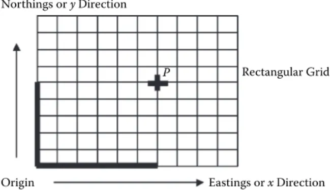
Points may then be located so far east (or to the right) of the origin and so far north (or up the page), using a standard unit of measure. The two distances are called the coordinates or more particularly the rectangular Cartesian coordinates (named after the French mathematician Descartes).
In Figure 1.2, the rectangular grid coordinates of P are (x, y) relative to the ori- gin and are shown here as (6, 5). The idea can be extended to three dimensions by adding the height above the origin. Although in some countries the x-direction is taken as being to the north or upward, here we will follow the convention that the direction across the page is the x-direction while up the page is described as the y-direction (x, y, or “in the door and up the stairs,” which is the opposite of many computer software graphics packages that measure the position of points from the top of the screen downward). Height is then in the z-direction. For any point on a three-dimensional object the coordinates would be (x, y, z). For two-dimensional (“flat Earth”) displays, z = 0.
Simple mathematical techniques can be used to analyze the locations of points that have been referenced to a rectangular grid. Sometimes it is useful to use a non- rectangular or skewed grid, for example, when trying to show three dimensions on a flat piece of paper (Figure 1.3). Data manipulation is slightly more complicated in these circumstances although the underlying principles are the same.
An alternative way of measuring the location of a point is through the use of polar coordinates (Figure 1.4). These describe points by their distance from an origin and their direction relative to some reference line. The direction is known as the bearing
P Rectangular Grid
Eastings or x Direction Origin
Northings or y Direction
FIGURE 1.2 Rectangular Cartesian coordinates.
z
y
x FIGURE 1.3 Nonrectangular or skewed grid.
and is normally measured clockwise from the north (or up the page). In Figure 1.4, P has polar coordinates (θ, d) relative to the origin, d being the distance, and θ (the Greek letter “theta”) being the direction or bearing from the north.
Angles and distances are examples of measures on the ratio scale. Distances are normally expressed as a ratio, for instance, between the amount of space between two points in comparison with a standard length. Under the Systeme International (SI) the standard unit of length is known as the metre and was once defined as the distance between two marks on a bar of platinum kept at constant temperature in Paris. It is now defined by stipulating that the speed of light is 299,792,458 meters (or “metres”) per second. As we will show later, trigonometrical formulae allow polar coordinates (θ, d) to be converted into Cartesians (eastings and northings or x and y) and vice versa.
Angles are a ratio between the amount of turning and a complete turn. They may be expressed as a proportion of either 360 degrees—written as 360° with each degree being subdivided into 60 minutes (60') and each minute into 60 seconds (60");
or 400 grads (where 100 grads equates with a quarter turn, with submeasurements being expressed as decimals) or 2π (two pi) radians where “pi” is the ratio between the diameter of a circle and its circumference.
Angular measures are important in surveying where positions may be expressed as if the Earth were a sphere using what are known as spherical coordinates. The latitude of a point is its angular distance north or south of the equator and is often represented by the Greek letter “phi” or ø. The longitude of a point is an angular measure east or west of the Greenwich standard meridian: it is normally represented by the Greek letter “lambda” or λ (see Figure 1.5).
The altitude or height of any point is measured as a distance above a reference level or surface, such as a mathematical shape that best approximates to the size and shape of the Earth. It is not normally given a Greek letter and hence the coordinates of points are either expressed as (ø, λ) or as (ø, λ, H). The use of Greek letters is common in mathematics. The full alphabet is given in Table 1.2.
For more accurate work, rather than assuming that the Earth is a perfect sphere, its shape is taken to be an ellipsoid (an ellipse rotated on its shorter axis creating a squashed sphere) as discussed in Chapter 4. However, for many practical purposes, the Earth can be regarded as a sphere. The word accurate as used here relates to nearness to the truth. The word precision will be used to refer to the exactness with
North
P
Length = d Origin
Angle θ
FIGURE 1.4 Polar coordinates.
which a value is expressed, whether the value is right or wrong. The word precision is often used to describe the number of decimal places that represent the quantity—
for example, a distance expressed as 2.105 m (where “m” means meters) is more pre- cise than 2 m though the latter may be nearer to the truth and hence more accurate.
On a flat surface, a straight line represents the shortest distance between two points. On a curved surface such as a sphere, a so-called straight line bends with the surface while a line of sight is even more bent because the light is refracted in the
N
P
O
G G´
Ø λ
λ
M
S
Parallel of Latitude
Equator
GG´ is the Greenwich Meridian of Origin (Zero Longitude) GM is the Equator (Zero Latitude)
O is the center of the spherical Earth The angle GOM is the longitude of P = λ
The angle MOP is the latitude of P = Ø FIGURE 1.5 Latitude and longitude.
TABLE 1.2
The Greek Alphabet
Letter Name Letter Name Letter Name
Α α alpha Ι ι iota Ρ ρ rho
Β β beta Κ κ kappa Σ σ sigma
Γ γ gamma Λ λ lambda Τ τ tau
Δ δ delta Μ μ mu Υ υ upsilon
Ε ε epsilon Ν ν nu Φ ø phi
Ζ ζ zeta Ξ ξ xi Χ χ chi
Ηη eta Ο ο omicron Ψψ psi
Θ θ theta Π π pi Ω ω omega
atmosphere. We will not deal with the consequences of the latter effect. In Chapter 11, we will consider how to transform measurements on curved surfaces onto a plane through map projections. Before doing so, measurements taken on the surface of the Earth need to be adjusted so that they fit on a mathematical surface known as the spheroid or ellipsoid of reference that is the best approximation to mean sea level.
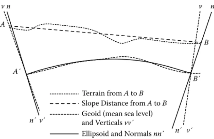
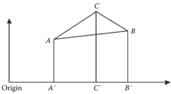
The surface defined by the mean level of the seas, assuming that they extend under the mountains, is known as the geoid. The difference in length between what is mea- sured and what is calculated is important in geodesy, which is the scientific study of the size and shape of the Earth. Figure 1.6 illustrates how the vertical as shown by a plumb line (here the lines vv′) may not in practice point at the center of the Earth (the lines nn′ are perpendicular to the mathematical surface A′B′) due, for example, to it being pulled aside by nearby mountains. We will discuss some of these matters later but for now we will focus on a flat Earth and two-dimensional representations.
Geographic information systems handle lines either as vectors or rasters. A vector is a quantity that represents both direction and distance. A polar coordinate as described above is an example of a vector quantity. Every straight line has a direc- tion and length (such as A to B in Figure 1.7) while a curved line may be considered as being made up of a series of short lines or vectors. In Chapter 8, there is further discussion on vectors.
On the other hand, a line can be considered as a series of points adjacent to each other, each point being of small but finite size (Figure 1.8). A television screen or a dot matrix printer produces what to the eye may appear like smooth curved lines but
Terrain from A to B
B n v n
v
B´
v´
n´
A
A´
v´
n´
Slope Distance from A to B Geoid (mean sea level) and Verticals vv´
Ellipsoid and Normals nn´
FIGURE 1.6 Straight-line distances.
B A
FIGURE 1.7 Lines as vectors.
which in practice are a series of points on a grid. Such a representation is called a raster image and each small square is known as a pixel.
Raster imaging can be used to show lines or areas. Raster data are simple for a computer to handle, but require relatively large amounts of computer storage. Given an area 20 cm by 20 cm and a grid cell size or resolution of 100 dots to the centimeter (i.e., one tenth of a millimeter) there will need to be a storage capacity for four mil- lion bits of information. For each vector it is necessary to record only the coordinates of the start and end points of straight-line sections.
One of several advantages of pixelation is that each pixel can be allocated a num- ber or set of numbers that indicate the characteristics of the point concerned. Those numbers may represent the color of the point, such as the proportion of red, green, and blue (referred to as RGB) to be used on a color television; or they may, for instance, represent the various wavelengths in the electromagnetic spectrum that have been picked up by a scanner, for example, in remote sensing. The values can either be analyzed through “number crunching” on a computer or they can be dis- played visually as an image that the human brain can analyze and interpret.
A line on a flat surface may be regarded as an item in its own right; alternatively, it may be regarded as the division between two areas: one on the left and the other to the right of the line. Topology involves the study of adjacency, that is, what lies beside a given area, containment (what is contained within it), and connectivity (how lines or areas are connected to other lines or areas).
Thus, in Figure 1.9, the area B is adjacent to the area A while the area C is con- tained within the area A. Point P is connected to point Q. The fact that the line PQ may be straight or curved is of no significance; what is important is that there is a division and areas A and B lie on opposite sides of it. Whether something belongs to one group or another is often an important consideration in mathematics and a specific form of symbolism or shorthand has been developed to analyze this, known as set theory.
As shown in Table 1.1, points, lines, and areas (and volumes) have size, shape, and location and also a classification. They each form part of a set of information.
A set, also called a class, is a collection of related objects that can be treated as an FIGURE 1.8 A line as a raster image.
entity in its own right. A set may be finite in size, such as the letters in an alphabet, or infinite, such as the set of integers that has no limit. A set is often identified by a pair of curved brackets such as (all human beings) or if they are in a specific sequence, angled brackets <letters in the Roman alphabet>. The symbol “∈” is used to indicate that an object is a member of a specified set {“a” ∈ < Roman alphabet >} while ∉ indicates that the object is not a member {“6” ∉ < Roman alphabet >}.
“A ⊂ B” shows that set A is a subset of set B (and “A ∉ B” that A is not a subset) while “A ⊃ B” means that set A includes set B. “A ∪ B” is the union of sets A and B, that is, it is the combination of set A and set B, the symbol “∪” sometimes being referred to as cup while “∩,” sometimes referred to as cap, is the intersection of A and B. See Figure 1.10.
We will not develop the ideas of topology nor the processes of classifying data, although we will be concerned with the outcomes of such classification when, in Chapters 12 and 13, we touch on elementary statistical techniques commonly used in geomatics and GIS. Throughout this book we will focus on two and three dimen- sions (length, breadth, and height, or latitude, longitude, and altitude) and how rel- evant data may be manipulated. Time is, of course, a further dimension and strictly
P
B A
C
Q FIGURE 1.9 Topology.
A
Set A Set B
B A B
FIGURE 1.10 Union and intersection of data sets A and B.
speaking we should consider not only the (x, y) or (x, y, z) coordinates of a point but also the (x, y, z, t) where t is time. Also, from a mathematical perspective, there is no inherent reason why we should not consider a world in which there are many more dimensions but this is outside the scope of the present book. Here, we will concen- trate on the manipulation of numbers that represent either location or the quantities found at a location.
SUMMARY
Absolute value: The value of a quantity for which there is an absolute zero and hence the quantity can be measured irrespective of its relation to other val- ues. It is also used in mathematics as the magnitude of a number without regard to whether it is positive or negative.
Accuracy: The nearest to truth or correctness of a quantity. Distinguished from precision, which relates to the exactness of a quantity regardless of whether it is nearer to the truth.
Adjacency: A term used in topology for areas that are side by side.
Bearing: The direction of an object, normally quoted as an angle measured clock- wise relative to the direction of north.
Cartesian coordinates: Numbers that indicate the distance from an origin and in directions parallel to two or three fixed lines known as the axes.
Categorical data: Data that are identified by their category or class.
Connectivity: A term used in topology to describe which lines or areas are connected to each other.
Containment: A term used in topology to describe objects within a given area or volume.
Continuous variable: A quantity that can take any intermediate value and is not restricted, for instance, to being an integer.
Data: Raw facts that have not been processed into information.
Decimal: A number that relates to a tenth part (or hundredth or thousandth, etc.), part of a whole number or integer.
Decimal places: The number of digits to the right of a decimal point.
Decimal point: A symbol after an integer that indicates the start of a series of deci- mal numbers. Here, a full stop (.) or period is used while in some countries a comma (,) is adopted. Thus, one thousand will be shown as 1,000.00 rather than 1.000,00.
Discrete variable: A quantity that can only take one of a distinct set of values such as an integer.
Distance: The amount of space between two points, often though not necessarily measured in a straight line.
Eastings: The distance in a Cartesian coordinate system east from an origin.
Ellipsoid: A mathematical shape that is, in effect, a squashed sphere and is a better approximation to the shape of the Earth than a pure sphere.
Equator: An imaginary line on the surface of the Earth that is equidistant from the North and South Poles.
Geodesy: The scientific study of the size and shape of the Earth.
Geoid: The shape of the Earth based on mean sea level and its imagined extension under or over land.
GIS: Geographic Information System (GIS) that is used to record, analyze, manipu- late, and display information, which relates to some location.
Great circle: A line on the surface of a sphere where the plane that contains the line passes through the center of the sphere.
Information: Data that have been processed and presented in a form that permits decisions to be made.
Integer: A whole number such as 1, 2, 3, 4, and so on.
Intersection: Those elements of two or more data sets that overlap.
Interval data: A set of discrete variables that take values at set intervals.
Latitude: The angular distance of a point north or south of the equator.
Longitude: The angular distance of a point on the Earth’s surface that is east or west of a meridian of origin, usually taken as the meridian through Greenwich in England.
Meridian of longitude: A great circle on the Earth’s surface that passes through the North and South Poles and a given point.
Nominal data: Data that are identified only by their class or category, such as apples or pears.
Northings: The distance in a Cartesian coordinate system north from an origin.
Numerical data: Data that are expressed in terms of numbers.
Ordinal data: Data that can be arranged in a sequence, such as preferences.
Origin: A fixed point that is the start point for a coordinate system from which east- ings and northings can be measured.
Parallel of latitude: A small circle on the Earth’s surface along the line of which all points have the same latitude.
Pixel: The smallest area on a display screen that can be uniquely identified.
Polar coordinates: A coordinate system based on the measurements of bearing and distance, the latter being either the straight-line distance or, on a sphere, the distance along a great circle.
Precision: The exactness of a quantity, for instance, the number of decimal places to which the quantity is expressed.
Raster: A rectangular pattern of parallel lines that divides a screen up into a series of pixels.
Ratio scale data: Data that are continuous and absolute.
Rectangular coordinates: Cartesian coordinates in which the axes are at right angles.
Small circle: A line on the surface of a sphere where the plane that contains the line does not pass through the center of the sphere.
Spherical coordinates: The location of points based on the angular measurements of latitude and longitude.
Topology: The study of geometric properties and relationships that are not related to their size or shape.
Union: The combination of two data sets.
Vector: A quantity that has direction as well as magnitude. (The term is also used for a matrix that has only one row or one column—see Chapter 7.)
13
2 Numbers and
Numerical Analysis
2.1 THE RULES OF ARITHMETIC
The mathematics that underpins all geographical analysis involves the application of rules, most of which are straightforward. Mathematics makes use of symbols, the most basic of which are shown in Table 2.1. We will add and explain other symbols later. In this chapter we will consider arithmetic, which is concerned with numerical calculations such as adding, subtracting, multiplying, and dividing.
The whole of arithmetic is based essentially on seven axioms, as shown in Box 2.1. Outside arithmetic, these axioms may not apply, for instance, when two raindrops running down a windowpane come together to make one raindrop so that in symbolic form: 1 + 1 = 1. Furthermore, computer programmers often write
“N = N + 1,” meaning “Take the number in the box labeled N, add one to that number and put it back in the box labeled N”; although partially an arithmetic operation, the use of the “=” sign has a different meaning from that which we are considering here.
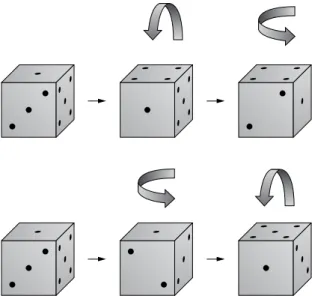
Axiom 1 in Box 2.1 states that adding a to b has the same result as adding b to a or in symbolic form, a + b = b + a, for instance, 2 + 5 = 5 + 2. This applies to basic arithmetic but elsewhere the sequence of operations is important. If you rotate a dice forward and then sideways it will finish in a different position than if you rotate it sideways and then forward (see Figure 2.1). This illustrates how in some circum- stances the sequence of operations can be important and we will discuss this further in Chapter 7 in the context of what are called matrices.
In this chapter, we will deal with simple arithmetic for which the axioms in Box 2.1 are fundamental. They are all necessary but they are not quite sufficient.
Consider the calculation 2 + 3 * 4. A pocket calculator will show 2 + 3 equals 5;
then enter 4 and multiply to give the answer 20. On the other hand, 3 * 4 equals 12.
Adding 2 gives 14. The same sum done in a different order gives a different answer.
Hence, we must have rules of priority. The simplest way to handle this is to place brackets around the groups that are together. Thus, in the first case, we have (2 + 3)
* 4, while in the second case, we have calculated 2 + (3 * 4). We must distinguish between these two cases. This leads to Rule 2.1 in Box 2.2.
BOX 2.1 AXIOMS OF ARITHMETIC AXIOM 1: THE COMMUTATIVE LAW
For any numbers a and b,
a plus b has the same value as b plus a.
Also,
a multiplied by b has the same value as b multiplied by a.
Put into symbols,
a + b = b + a a * b = b * a The latter may also be written as
ab = ba AXIOM 2: THE ASSOCIATIVE LAW For any three numbers a, b, c,
(a + b) + c = a + (b + c) Also,
(ab)c = a(bc)
AXIOM 3: THE DISTRIBUTIVE LAW For any numbers a, b, c, then
a * (b + c) = a * b + a * c or
a(b + c) = ab + ac AXIOM 4
There is a number called zero (0) that for any a a + 0 = a TABLE 2.1
Standard Symbols
Add + Less than < Equal =
Subtract – More than > Nearly equal ≈
Multiply * Less or equal ≤ Not equal ≠
Divide / More or equal ≥
(Historically, there was a debate as to whether 0 was actually a number. The Romans, for example, used the symbols I, V, X, L, C, D, and M to represent 1, 5, 10, 50, 100, 500, 1000 in the decimal system but had no zero.)
AXIOM 5
There is also a number 1 such that
a * 1 = a AXIOM 6
For every value of a there is a number d such that a + d = 0
(This then introduces the whole range of negative numbers.) AXIOM 7
Provided c does not equal zero (c ≠ 0), then
if c * a = c * b then a = b
(Similarly, if a + c = b + c, then a = b although this also applies if c = 0 but not when c is infinitely large.)
FIGURE 2.1 Rotating a dice (forward + sideways or sideways + forward).
Where there are no brackets, then we have to decide which comes first—addition (+), subtraction (–), multiplication (*), or division (/). In fact, it does not normally matter whether we multiply and then divide in that order, or divide first and then multiply. Thus,
3 * 4/2 = (3 * 4)/2 = 12/2 = 6 while 3 * (4/2) = 3 * 2, which also equals 6.
The same happens with addition and subtraction. Thus, 2 + 3 – 4 = (2 + 3) – 4 = 5 – 4 = 1 while 2 + (3 – 4) = 2 – 1, which also equals 1.
When there is doubt, we should carry out the multiplication or division before the addition or subtraction. This leads to Rule 2.2 in Box 2.2.
Numbers may be positive or negative and when handling these, simple rules also apply. Thus, adding a negative number is the same as subtracting a positive while subtracting a negative number is the same as adding a positive. Put another way:
4 + (–3) = 4 – 3 = 1
while 4 – (–3) = 4 + 3 = 7.
Multiplication and division follow Rule 2.3 in Box 2.2.
BOX 2.2 RULES OF ARITHMETIC RULE 2.1
Place items that are together in brackets and deal with what is inside the brack- ets first.
RULE 2.2
If there are no brackets or when what is inside the brackets has been evaluated, then deal with multiplication or division before addition or subtraction.
RULE 2.3
(positive) * (positive) =+= (positive)/(positive) (positive) * (negative) = – = (positive)/(negative) (negative) * (positive) = – = (negative)/(positive) (negative) * (negative) =+= (negative)/(negative) RULE 2.4
To add or subtract fractions they must share a common denominator.