Bootstrapping fully-automatic temporal fetal brain segmentation in volumetric MRI time series

Bootstrapping Fully-Automatic Temporal Fetal

Brain Segmentation in Volumetric MRI Time Series

by

Lawrence Zhang

S.B., Computer Science

Massachusetts Institute of Technology (2018)

Submitted to the Department of Electrical Engineering and Computer

Science

in partial fulfillment of the requirements for the degree of

Master of Engineering in Electrical Engineering and Computer Science

at the

MASSACHUSETTS INSTITUTE OF TECHNOLOGY

June 2019

c

○ Massachusetts Institute of Technology 2019. All rights reserved.

Author . . . .

Department of Electrical Engineering and Computer Science

May 24, 2019

Certified by . . . .

Polina Golland

Professor

Thesis Supervisor

Accepted by . . . .

Katrina

LaCurts

Chair,

Master of Engineering Thesis Committee

Bootstrapping Fully-Automatic Temporal Fetal Brain

Segmentation in Volumetric MRI Time Series

by

Lawrence Zhang

Submitted to the Department of Electrical Engineering and Computer Science on May 24, 2019, in partial fulfillment of the

requirements for the degree of

Master of Engineering in Electrical Engineering and Computer Science

Abstract

We present a method for bootstrapping training data for the task of segmenting fetal brains in volumetric MRI time series data. Temporal analysis of MRI images requires accurate segmentation across frames, despite large amounts of unpredictable motion. We use the predicted segmentations of a baseline model and leverage anatomical structure of the fetal brain to automatically select the “good frames” that have accu-rate segmentations. We use these good frames to bootstrap further model training. We also introduce a novel temporal segmentation model that predicts segmentations using a history of previous segmentations, thus utilizing the temporal nature of the data. Our results show that these two approaches do not provide conclusive improve-ments to the quality of segmentations. Further exploration into the automatic choice of good frames is needed before reevaluating the effectiveness of the bootstrapping and temporal methods.

Thesis Supervisor: Polina Golland Title: Professor

Acknowledgments

I would like to thank my mentor and advisor, Professor Polina Golland, for the op-portunity of working on this project, as well as the guidance she provided throughout the research process. I would also like to express my gratitude to all of the members of the Golland Group for the countless times they helped debug, problem solve, and propose solutions. Special thanks to Esra Turk from the Boston Children’s Hospi-tal for the acquisition and organization of the dataset. Finally, I would not have completed this thesis without the amazing support from my family and friends.

Contents

3.3 Baseline U-Net Model . . . 22

3.3.1 Architecture . . . 22

3.3.2 Loss Function . . . 23

3.3.3 Prediction and Evaluation . . . 23

3.4 Bootstrapping . . . 24

3.5 Temporal Segmentation . . . 25

4 Results 27 4.1 Experiments . . . 27

4.3 Good Frames . . . 29

5 Discussion 33 5.1 Conclusion . . . 33

5.2 Future Work . . . 34

5.2.1 Identifying Good Frames . . . 34

5.2.2 Anatomical constraints . . . 35

A Data Augmentation Matrices 37 A.1 Rotation . . . 37

A.2 Translation . . . 38

A.3 Shearing . . . 38

List of Figures

1-1 Example of a singleton pregnancy case. The same cross-section from three consecutive frames is shown. Arrows indicate substantial motion in the fetal brain. . . 14 1-2 Cross-section of a fetal brain segmentation in a singleton pregnancy

case (a). All voxels that are part of the fetal segmentation have value 1 and are shown in white. The outline of the segmentation is overlayed in red on the original BOLD MRI image for easier readability (b). . . 15

2-1 The U-Net model architecture for a 96×96 pixel input image. Each blue box corresponds to a multi-channel feature map. The number of channels is indicated above the box, while the 𝑥 and 𝑦 dimensions are indicated at the lower left of the box. White boxes represent concate-nated featured maps. . . 18 2-2 Overview of ACNN architecture for a 96×96 pixel input image.

Out-put segmentation is generated as in the U-Net model (blue). This segmentation is passed through an encoder (green), where the result-ing encodresult-ing is used to regularize the model. . . 19

4-1 Segmentation predictions generated by each of the three models. Pre-dictions are illustrated in green, while the ground truth segmentation is shown in red. . . 28 4-2 Dice scores of segmentations generated by the baseline, bootstrapped,

and temporal models. Samples 1-7 are singleton pregnancies, and sam-ples 8-10 are twin pregnancies. . . 29

4-3 Comparison of per-series good frames percentage as determined by different models. Diagonal line represents no change (i.e. both models predict the same percentage of good frames for the given time series). 31

List of Tables

4.1 Average Dice scores of the train and tests sets of each of the three models. 28 4.2 Comparison of each model’s segmentation using metrics the frequency

and distribution of good frames. There are 31448 frames and 108 series total. . . 30

Chapter 1

Introduction

1.1

BOLD MRI

Blood oxygenation level dependent (BOLD) magnetic resonance imaging (MRI) is an imaging technique that is used to visualize and track changes in the oxygenation levels of various organs [12]. Particularly, BOLD MRI has uses in identifying the functional dynamics of the placenta, fetal brains, and other fetal organs [14, 15]. Because abnormalities in the transportation of oxygen from the placenta to the fetus are associated with perinatal mortality [7], tracking the changes in fetal and placental oxygenation levels in response to maternal oxygenation can be used to detect placental dysfunction [1]. Thus, quantitative analysis on BOLD MRI signals in fetal organs suggests a promising noninvasive method for monitoring both fetal and maternal health [14, 15].

BOLD MRI time series are sequences of three-dimensional BOLD MRI volumes (frames) taken over periods of time. While the added temporal dimension of the data allows for the quantitative analysis of changes in fetal and placental oxygenation between frames, it also causes the data to suffer from serious motion artifacts. Specifi-cally, movement from factors like maternal respiration, unpredictable fetal movement, and signal non-uniformities are tracked between frames of the series [16, 9]. Examples of some motion artifacts are illustrated in Figure 1-1. Additional complications arise from the fact that different organs move differently in the time series. Fetal brain

Figure 1-1: Example of a singleton pregnancy case. The same cross-section from three consecutive frames is shown. Arrows indicate substantial motion in the fetal brain.

movement can be modeled as rigid transformations [6, 17], but the placenta moves more locally and deforms non-rigidly. For some organs, the number of instances that the organ appears in the frames can also vary. For example, in twin pregnancies, there will be two fetal brains. Thus, acquiring accurate quantitative measures of BOLD MRI time series remains challenging.

1.2

Image Segmentation

In order to correctly quantify oxygenation levels in BOLD MRI images, accurate identification of organs and their boundaries is needed to precisely locate the fetal organs across different frames in the time series. One approach for finding the organs is to use image segmentation, which is the process of partitioning an image into different segments where each segment represents some higher-level feature. Here, each voxel in a frame is assigned a label of 1 that indicates if the voxel is part of an organ (e.g. fetal organ or placenta), or a label of 0 if it belongs to the background. An example fetal brain segmentation is shown in Figure 1-2. By segmenting every frame in a time series, we can then locate and track the organs over time.

Though image segmentation is essential for providing quantitative insight, the training of robust image segmentation models often requires large amounts of labeled data. Manual segmentation is extremely time-consuming because each frame in the

(a) (b)

Figure 1-2: Cross-section of a fetal brain segmentation in a singleton pregnancy case (a). All voxels that are part of the fetal segmentation have value 1 and are shown in white. The outline of the segmentation is overlayed in red on the original BOLD MRI image for easier readability (b).

MRI time series is a three-dimensional volume. Thus, the task of labeling sufficient data to train a robust model becomes infeasable. A common approach to artificially increase the amount of training data is to perform data augmentation, which consist of applying random transformations to the images and corresponding segmentations in the training set [11]. While data augmentation may help improve model performance, the transformations used may not fully capture all of the possible variation in the positions and orientations of organs in the frames.

In order to provide better segmentations of fetal organs, we explore a method of image segmentation that leverages the characteristics of the BOLD MRI time series data in addition to traditional data augmentation. Specifically, our segmentation pipeline will utilize the specific types of motion of the organs we are segmenting as well as the overall temporal nature of the data to produce robust segmentations of BOLD MRI images.

1.3

Thesis Outline

This thesis presents a novel approach for segmenting BOLD MRI time series data that incorporates aspects of the data to produce better segmentations. This thesis focuses on the segmentation of the fetal brain, which will provide a backbone for

future work in segmentation of other fetal organs and the placenta.

Chapter One describes the motivation and gives and introduction to image seg-mentation as a tool for quantitative analysis of MRI images. Chapter Two reviews three existing approaches for segmenting fetal organs. Chapter Three describes our approach, including both baseline models and the new segmentation pipeline. Chap-ter Four discusses the results of each model. ChapChap-ter Five draws conclusions and proposes topics for future work.

Chapter 2

Related Work

There are a few possible ways to generate segmentations on three dimensional MRI images. In this chapter, we present three existing methods.

2.1

U-Net

One approach for image segmentation is the use of deep convolutional neural net-works. In particular, the U-Net architecture has demonstrated promise for delivering fast segmentations with limited training samples [13]. The U-Net generates two-dimensional segmentations for two-two-dimensional input images. The network consists of two sections: a contracting section and an expanding section. The first is a series of convolutional and down-sampling layers, similar to a traditional convolutional neural network. The second consists of a symmetric series of convolutional and up-sampling layers. Intermediary features from the contracting section are combined with upsam-pled features in the expanding section to help with high resolution localization of the segmentation. This network architecture is illustrated in Figure 2-1.

In order to get accurate and robust segmentations with the U-Net and very little training data, excessive data augmentation is needed. In the original U-Net paper, elastic deformations are applied to available training images, allowing the model to learn invariance to these deformations without having explicit annotated examples. While data augmentation has been successful for learning invariance [4], the extent

Figure 2-1: The U-Net model architecture for a 96×96 pixel input image. Each blue box corresponds to a multi-channel feature map. The number of channels is indicated above the box, while the 𝑥 and 𝑦 dimensions are indicated at the lower left of the box. White boxes represent concatenated featured maps.

of its effectiveness is limited by how well the augmentation represents the variance in the input images.

Due to its simple design and success in image segmentation we will use the U-Net along with data augmentation as a baseline for our experiments.

2.2

ACNN

Because image segmentation provides labels at a per-pixel level, segmentation perfor-mance often suffers from artifacts in the image. The anatomically constrained neural network (ACNN) attempts to mitigate this by incorporating prior knowledge about the segmented organ’s shape and location [10]. The ACNN extends the base U-Net architecture by additionally training an autoencoder on segmentation labels. The en-coder part of the autoenen-coder is then used to regularize the output segmentations of the U-Net, encouraging the model follow the underlying anatomy of the image when generating the segmentations. This network architecture is illustrated in Figure 2-2. The effectiveness of the ACNN relies on the ability of the encoder portion of the network to provide a representative encoding of the segmentations. For some types of organs, such as the fetal brain, data augmentation is sufficient to train a robust

Figure 2-2: Overview of ACNN architecture for a 96×96 pixel input image. Output segmentation is generated as in the U-Net model (blue). This segmentation is passed through an encoder (green), where the resulting encoding is used to regularize the model.

autoencoder. This is because fetal brains are rigid in structure, and their anatomy can be easily represented using rigid affine transformations. However, this is not the case for many other organs. For example, the placenta is an extremely non-rigid organ, data augmentation alone is not sufficient to train an autoencoder that can effectively represent its underlying anatomy.

While this thesis focuses on the segmentation of fetal brain, we would like to even-tually address the segmentation of other organs, including the placenta. Since a large dataset of segmentations for placenta and other fetal organs is not available, we do not explore the ACNN in this thesis. However, incorporating anatomical constraints in future work is discussed in Section 5.2.

2.3

Temporal Registration

Another way of generating segmentations for each frame in an MRI series is to start from a manual segmentation of a reference frame, and then to propagate this seg-mentation over the rest of the frames in the series. One method of doing this uses a hidden Markov model (HMM) to model the temporal nature of the deformations between frames in the series [8]. Then, these deformations are applied to the reference segmentation to generate segmentations for all frames in the series.

The main drawback with this approach is that it requires a manually segmented reference frame to propagate. Thus, it only provides a semi-automatic solution for segmenting MRI time series. Additionally, separate HMMs must be used to learn the

deformations for different time series, so there is also a very large time overhead for determining the segmentations of new MRI scans.

We desire a framework that is both fully automatic and capable of generating segmentations quickly without having to retrain on new data. While the tempo-ral registration method provides neither, we can utilize the notion of propagating segmentations in order to leverage the temporal aspect of the time series data.

Chapter 3

Methods

In this chapter, we describe our dataset and outline our approach for training a fully automatic model that generates segmentation of the fetal brain in MRI time series.

3.1

Data

BOLD MRI scans of pregnant women are acquired on a 3T Skyra Siemens scanner using 3×3mm2 in-plane resolution, 3mm slice thickness, and interleaved slice acquisi-tion. The scans include 87 singleton pregnancies and 21 twin pregnancies (108 total), all between 28 and 37 weeks of gestational age.

Each of the 108 time series contain between 50 and 350 volumes, each with between 48 and 96 slices. To eliminate slice interleaving effects, we split the even and odd slices of each volume into separate volumes, and then perform linear interpolation between the slices of these separated volumes. This effectively doubles the number of frames in the series, yielding a total of between 100 and 700 volumes for each series. For quantitative evaluation, we manually segment the fetal brains in a randomly chosen volume in 60 of the time series (50 singleton and 10 twin series). While this gives us a total of 70 segmented brains, we do not differentiate between brains in twin pregnancies so that our segmentation problem remains as a per-voxel binary classification. We split these 60 volumes into a training set of 50 samples (43 singleton, 7 twin) and a test set of 10 samples (7 singleton, 3 twin).

3.2

Data Augmentation

Since we only have access to 60 manually segmented frames, we perform significant data augmentation in order to artificially increase our training data size. In order for our data augmentation to be effective, we must randomly apply transformations to our training set that are representative of possible variation in the location, orienta-tion, and shape of fetal brains. As mentioned in Section 1.1, fetal brains are rigid in structure, and thus can be modeled using rigid affine transformations. Specifically, we randomly rotate, translate, shear, scale, and crop the volumes. Since these trans-formations may include voxels originally outside the boundaries of the original image, we interpolate the values of these voxels by taking the value of the nearest voxel from the original image. This ensures that the interpolated voxels have statistics that roughly resemble those of the background in the original image. Appendix A lists the matrices used to perform these random transformations.

3.3

Baseline U-Net Model

3.3.1

Architecture

We modify the original U-Net architecture to function with three-dimensional volume inputs. The architecture is virtually the same as illustrated in Figure 2-1, but with the added dimension. Specifically, the input image and output segmentation are single-channel volumes with dimensions 96×96×48. All feature maps now have four dimensions—𝑥, 𝑦, 𝑧, and channel. Convolutional layers are 3×3×3 and max pooling layers are 2×2×2. As in the original network, the number of feature channels is doubled after each downsample, and upsampled feature maps are concatenated with the corresponding downsampled feature maps in order to recover border voxels and retain resolution. The only modification we make to the network is that we replace up-convolution layers with 2×2×2 transpose convolutional layers [5], as they make implementation easier. Like the two-dimensional U-Net, this network has a total of 23 convolutional layers.

3.3.2

Loss Function

The volume of the fetal brain is considerably small compared to the volume of the entire frame. Thus, we use a weighted crossentropy loss function for training the U-Net. In addition, to ensure that the predicted segmentation closely captures the ridges and grooves of the structure of the fetal brain, we add additional weight to the loss for voxels close to the boundary of the manual segmentation. These boundary voxels are easily calculated by performing a 3×3×3 average pooling on the label, and then identifying the voxels with values that are neither 0 nor 1. Thus, the loss function between label 𝑦 and prediction ˆ𝑦 is

ℒ(𝑦, ˆ𝑦) = −[𝑤𝑠𝑦 log ˆ𝑦 + (1 − 𝑦) log 𝑤𝑏(1 − ˆ𝑦)][1 + 𝜆1(0 < 𝐽3* 𝑦 < 1)] (3.1)

where 𝑤𝑠 and 𝑤𝑏 are the segmentation and background class weights, respectively,

𝜆 is the boundary weight parameter, 1 is the indicator function, 𝐽3 is the 3×3×3

matrix of all-ones, and * is the convolution operator.

3.3.3

Prediction and Evaluation

Since we restrict the input size of the U-Net to be a 96×96×48 volume and most of our volumes are larger than this, our model is only capable of predicting the segmentation for part of a full volume at once. In order to predict the segmentation for an entire volume, we first split the volume into 8 (potentially overlapping) sections of the input size (96×96×48), one in each corner of the original volume. We use the network to generate segmentations for each of these 8 sections, then combine the predictions into one segmentation, averaging any overlapping voxels.

The loss function described in Section 3.3.2 is determined individually for each of the 8 sections of size 96×96×48. However, we evaluate the performance of our model by calculating metrics on the combined prediction. Specifically, we determine the Dice coefficient [3] to quantify the voxel-wise volume overlap between the combined segmentation and the manual segmentation.

3.4

Bootstrapping

We use our trained U-Net to generate segmentation predictions for every frame of every series in our dataset (all 108 time series). While the model will likely provide accurate segmentations for some of the frames, it is unlikely that it will succeed for every one. However, we can bootstrap additional training by including those accurately predicted segmentations in our training set. In order to ensure that this bootstrapping process is fully-automatic, we must be able to identify these “good frames” without human input.

To do this, we leverage some of the anatomy of fetal brains. Because the brains are rigid in structure, their volumes will fluctuate very little, even if there is a lot of movement between frames. Thus, we make the assumption that if a predicted segmentation has a volume that is within 5% of the manual segmentation’s volume, it can be considered a good frame. If no manual segmentation is available, the predicted segmentation must have a volume within 10% of the average single fetal brain volume of around 11100 voxels, as well as within 5% of the segmentation volumes of the previous and next frames. Overall, our accepted margin of error is around ±555 voxels. Since the average surface area of a single fetal brain is around 2400 voxels, we believe that our margin of error is sufficiently small. It is important to note, however, that our assumption is likely oversimplified, as it is possible for a predicted segmentation to be inaccurate but still have a volume within our margin. We address potential improvements to this step in Section 5.2.

After determining all of the good frames for each time series, we then train a new model using a subset of the good frames as our training data. Specifically, we determine the time series with over 60% good frames and remove any series in our original test set. To ensure that the model is not biased towards the training series with more good frames, we sample from each training series uniformly. To evaluate the effectiveness of our bootstrapping, we compare the Dice score of the predictions from this new model with those from our baseline. We also determine if there is an increase in the number of good frames using the predictions generated by this new

model.

3.5

Temporal Segmentation

In addition to using these good frames for bootstrapping a U-Net, we can also use them in a model that leverages the temporality of the data. The current U-Net model uses a single frame as input to predict its segmentation. If we also include previous frames and their segmentations in our input, the model can use information on past segmentations in the series to help make its prediction. Due to memory constrains, we limit the input to only include the single preceding frame and its segmentation. Thus, our new temporal model is simply a U-Net with a three-channel input volume of size 96×96×48×3.

This dataset can easily be created by taking a subset of our bootstrapped frames training set. We use all consecutive pairs of good frames such that, for frame 𝑥 and predicted segmentation ˆ𝑦 at time 𝑡, our new input is the concatenation of (𝑥𝑡−1, ˆ𝑦𝑡−1, 𝑥𝑡) and our new label is ˆ𝑦𝑡. It is important to note that the motion between

frames can realistically happen in reverse, so we also include input (𝑥𝑡, ˆ𝑦𝑡, 𝑥𝑡−1) and

label ˆ𝑦𝑡−1in the new dataset. Again, during training we sample each series uniformly.

Like the temporal registration approach described in Section 2.3, this model re-quires already having a segmentation for one frame in order to predict segmentations for the entire time series. We use the output of our baseline U-Net on the first frame in the series as our starting segmentation, and then propagate it forward in time us-ing our temporal model. We then evaluate the performance of our temporal network using the same test set from the baseline.

Chapter 4

Results

This chapter presents a comparison of the performance of each of the baseline, boot-strapped, and temporal U-Net models, as presented in Chapter 3.

4.1

Experiments

The baseline U-Net was trained for 3000 epochs with a training set size of 50 frames. We used this model to generate predictions for all frames in all time series and iden-tify the good frames. We then used around 18000 of the good frames to train the bootstrapped U-Net for 15 epochs. Around 12000 pairs of consecutive good frames were used to train the temporal model for 15 epochs. For all three models, boundary weight 𝜆 = 1, and class weights 𝑤𝑠 and 𝑤𝑏 were automatically determined based on

the training set (see Equation 3.1).

4.2

Segmentation

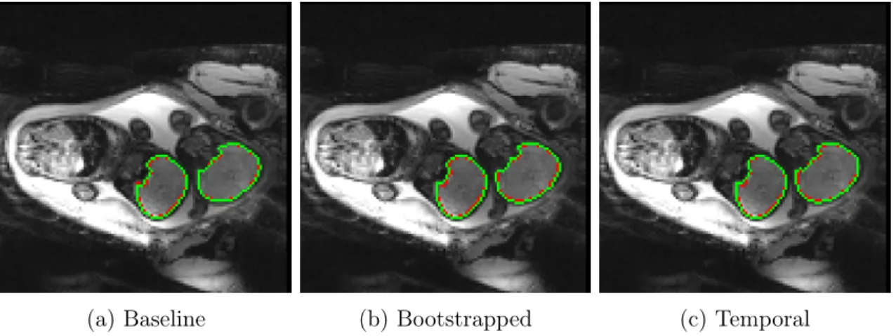
All three models were evaluated with the same test set of 10 labeled frames (7 singleton and 3 twin). Figure 4-1 depicts the predictions made by the three models on the same frame from a twin pregnancy sample in the test set. The Dice scores for this sample were 0.9578, 0.9417, and 0.9464 for the baseline, bootstrapped, and temporal models, respectively. Note that Dice scores for twin samples are calculated using the combined

(a) Baseline (b) Bootstrapped (c) Temporal

Figure 4-1: Segmentation predictions generated by each of the three models. Pre-dictions are illustrated in green, while the ground truth segmentation is shown in red.

Baseline Bootstrapped Temporal Train Dice 0.9643 0.9273 0.9373

Test Dice 0.8865 0.8984 0.8794

Table 4.1: Average Dice scores of the train and tests sets of each of the three models.

segmentation of both brains, and not for each brain individually. Visually, all three models predict very similar segmentations that are all very close to the ground truth segmentation.

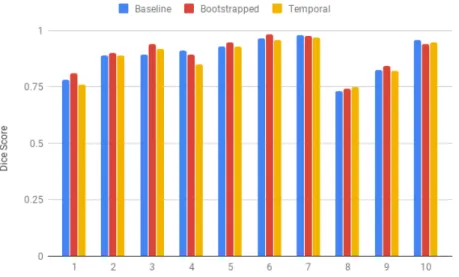
The Dice scores of the segmentations for each of the 10 frames in the test set are illustrated in Figure 4-2. The segmentations from Figure 4-1 correspond to sample 10. Again, all three models perform similarly over the 10 test set samples.

Table 4.1 summarizes the average Dice score during training and testing for each of the three models. Both the bootstrapped and temporal models have much lower training Dice scores compared to that of the baseline. This is likely due to the much larger training sets used to train these two models. Despite this, the resulting average test set Dice score is roughly the same for all three models.

Thus, in terms of quality of segmentation in the test set, the bootstrapped and temporal U-Net models perform comparably to the baseline U-Net. However, this set of data is extremely small and consists of only a single frame per series. Thus, comparing predictions with the ground truth cannot provide a completely accurate

Figure 4-2: Dice scores of segmentations generated by the baseline, bootstrapped, and temporal models. Samples 1-7 are singleton pregnancies, and samples 8-10 are twin pregnancies.

representation of how each network performs in segmenting an entire series of MRI images. As it is impractical to manually segment an entire series in order to measure model performance, we utilize our definition of a good frame to help quantify the effectiveness of each network.

4.3

Good Frames

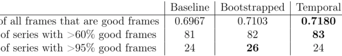
Since we do not have labels for every frame in a series, we instead use the amount of good frames as an indication of each models’ segmentation performance. We look at two metrics: the percent of all 31448 frames in the dataset (including test set samples) that are good frames, and the distribution of percentage of good frames per time series. A summary of these results is displayed in Table 4.2. Ideally, a model that performs better than our baseline will have a higher value in all three rows. However, this does not seem to be the case, as all three models seem to be performing similarly. Overall, the bootstrapped and temporal models generate around 500 more good frames than the baseline model. While this is not a substantial increase, it is worth investigating which samples are being better segmented. To do this, we compare

Baseline Bootstrapped Temporal % of all frames that are good frames 0.6967 0.7103 0.7180

# of series with >60% good frames 81 82 83 # of series with >95% good frames 24 26 24

Table 4.2: Comparison of each model’s segmentation using metrics the frequency and distribution of good frames. There are 31448 frames and 108 series total.

the percentages of good frames per time series of the bootstrapped and temporal models against those of the baseline. For example, if a model is predicting more frames correctly in a series, then the percentage of good frames in that series will increase. Likewise, if a model is performing worse, the percentage of good frames will decrease. Comparisons of the changes in per-series good frame percentages between the bootstrapped and baseline models and between the temporal and baseline models are illustrated in Figure 4-3. All points above the diagonal line are time series with more good frames as a result of the non-baseline model.

In general, there was no significant changes in amount of good frames for the majority of the time series. However, the bootstrapped model did seem to generally improve the number of segmentations in the series that had fewer baseline good frames: note how all the series with fewer than 40% good frames from the baseline model all had more using the bootstrapped model. The temporal model, however, showed both large increases and decreases for various series.

(a) Bootstrapped vs. Baseline

(b) Temporal vs. Baseline

Figure 4-3: Comparison of per-series good frames percentage as determined by dif-ferent models. Diagonal line represents no change (i.e. both models predict the same percentage of good frames for the given time series).

Chapter 5

Discussion

Finally, we discuss the significance of our results and the limitations of our methods, and propose future improvements.

5.1

Conclusion

Image segmentation is a powerful tool that allows for quantitative analysis of MRI time series data. However, current approaches for automatically generating these segmentations rely on large amounts of labeled data, which is often impractical to ac-quire. In this thesis, we present a bootstrapping method for automatically generating more training data, and then apply this to a new temporal segmentation network. These new approaches attempt to leverage the underlying anatomy and temporality of the time series data in order to generate more accurate segmentations.

As illustrated in our results, however, neither the data bootstrapping nor the temporal network seem to significantly affect the quality of the segmentations. While both methods seem to slightly improve the number of frames in the time series that are properly segmented, this change is extremely small compared to the total size of the data (<1%).

However, these results are not fully indicative that these two new methods should not be explored further, as the results are reliant on a fairly large assumption made in the bootstrapping process. As discussed in Section 3.4, we assume that as long as

a segmentation has a volume within a certain margin, it is considered a good frame. This margin is arbitrarily chosen, and thus it is very likely that the automatically selected good frames is not representative of the actual set of correctly generated segmentations. Specifically, is it possible for an incorrect segmentation to have a “correct” volume, and even more likely for a correct segmentation to have an “incor-rect” volume. As a result, the training set used for the bootstrapped and temporal models are likely skewed, thus resulting in little improvement from the baseline. This assumption clearly needs to be refined, and the next section discusses one possible approach for doing so.

5.2

Future Work

5.2.1

Identifying Good Frames

An alternative approach for determining good frames that was explored during exper-imentation was to limit both the volume of the segmentation and the overlap of the segmentations between consecutive frames. While this would reduce the likelihood of including incorrect segmentations, it also limits the amount of motion variance in the good frames dataset. Thus, we need to identify a constraint that can easily identify good segmentations, even with large motion.

One possible future approach borrows from the registration technique presented in the temporal registration paper [8]. Accurate segmentations over time will follow the rigid transformation assumption used on fetal brains. Thus, good frames can be identified by testing if a segmentation falls within an allowable margin of affine transformations from the previous frame. Like the temporal registration method, this approach will be significantly more time consuming to calculate. However, this only needs to be performed once to generate the bootstrapped data, and will not need to be performed for every new time series.

5.2.2

Anatomical constraints

Section 2.2 introduced anatomical constraints to help regularize the segmentation network. In addition to testing the original ACNN architecture proposed in the paper, we also propose a novel double-U-Net architecture. Unlike the ACNN, which regularizes the output of the U-Net, the double-U-Net would regularize the lowest resolution feature map. The contracting section of the U-Net doubles as an encoder, and decoder is added that generates a replica of the input image. This autoencoder would thus force this feature map to encode structural information regarding the MRI image.

Both the ACNN and double-U-Net may help produce more accurate segmenta-tions by further constraining the segmentasegmenta-tions that are produced. They can also be combined with the bootstrapping and temporal approaches proposed in this thesis to potentially improve segmentation accuracy.

Appendix A

Data Augmentation Matrices

All transformation matrices are applied to three-dimensional volumes with an addi-tional channel dimension (four dimensions total).

A.1

Rotation

The matrices for a rotation of 𝜃𝑖 about the 𝑖-axis are

𝑅𝑥 = ⎡ ⎢ ⎢ ⎢ ⎢ ⎢ ⎢ ⎣ 1 0 0 0 0 cos 𝜃𝑥 − sin 𝜃𝑥 0 0 sin 𝜃𝑥 cos 𝜃𝑥 0 0 0 0 1 ⎤ ⎥ ⎥ ⎥ ⎥ ⎥ ⎥ ⎦ (A.1) 𝑅𝑦 = ⎡ ⎢ ⎢ ⎢ ⎢ ⎢ ⎢ ⎣ cos 𝜃𝑦 0 sin 𝜃𝑦 0 0 1 0 0 − sin 𝜃𝑦 0 cos 𝜃𝑦 0 0 0 0 1 ⎤ ⎥ ⎥ ⎥ ⎥ ⎥ ⎥ ⎦ (A.2) 𝑅𝑧 = ⎡ ⎢ ⎢ ⎢ ⎢ ⎢ ⎢ ⎣ cos 𝜃𝑧 − sin 𝜃𝑧 0 0 sin 𝜃𝑧 cos 𝜃𝑧 0 0 0 0 1 0 0 0 0 1 ⎤ ⎥ ⎥ ⎥ ⎥ ⎥ ⎥ ⎦ (A.3)

𝜃𝑖’s are sampled uniformly at random between −𝜋 and 𝜋. Note that these matrices do

not sample all possible three-dimensional rotations uniformly. A uniform alternative can be found in [2]. However, we assume that the added bias is negligible.

A.2

Translation

The matrix for a translation of 𝑡𝑖 in the 𝑖 direction is

𝑇 = ⎡ ⎢ ⎢ ⎢ ⎢ ⎢ ⎢ ⎣ 1 0 0 𝑡𝑥 0 1 0 𝑡𝑦 0 0 1 𝑡𝑧 0 0 0 1 ⎤ ⎥ ⎥ ⎥ ⎥ ⎥ ⎥ ⎦ (A.4)

𝑡𝑖’s are sampled uniformly at random between -0.1 and 0.1 times the size of the

𝑖-dimension of the input.

A.3

Shearing

The matrix for a sheer of ℎ𝑗_𝑖 in 𝑖 in the 𝑗 direction is

𝐻 = ⎡ ⎢ ⎢ ⎢ ⎢ ⎢ ⎢ ⎣ 1 ℎ𝑦 𝑥 ℎ𝑧𝑥 0 ℎ𝑥 𝑦 1 ℎ𝑧𝑦 0 ℎ𝑥_𝑧 ℎ𝑦_𝑧 1 0 0 0 0 1 ⎤ ⎥ ⎥ ⎥ ⎥ ⎥ ⎥ ⎦ (A.5)

A.4

Scaling

The matrix for scaling the image by a factor 𝑠𝑖 with respect to 𝑖 is

𝑆 = ⎡ ⎢ ⎢ ⎢ ⎢ ⎢ ⎢ ⎣ 𝑠𝑥 0 0 0 0 𝑠𝑦 0 0 0 0 𝑠𝑧 0 0 0 0 1 ⎤ ⎥ ⎥ ⎥ ⎥ ⎥ ⎥ ⎦ (A.6)

Bibliography

[1] S. Aimot-Macron, L.J. Salomon, B. Deloison, R. Thiam, C.A. Cuenod, O. Clement, and N. Siauve. In vivo MRI assessment of placental and fetal oxygenation changes in a rat model of growth restriction using blood oxy-gen level-dependent (BOLD) magnetic resonance imaging. European Radiology, 23(5):1335–1342, 2013.

[2] J. Arvo. Fast random rotation matrices. Graphics Gems III, 1991.

[3] L.R. Dice. Measures of the amount of ecologic association between species. Ecol-ogy, 26(3):297–302, 1945.

[4] A. Dosovitskiy, J.T. Springenberg, M. Riedmiller, and T. Brox. Discriminative unsupervised feature learning with convolutional neural networks. In Neural Information Processing Systems, 2014.

[5] V. Dumoulin and F. Visin. A guide to convolution arithmetic for deep learning. 2016.

[6] G. Ferrazzi, M.K. Murgasova, T. Arichi, C. Malamateniou, M.J. Fox, A. Makropoulos, J. Allsop, M. Rutherford, S. Malik, P. Aljabar, and J.V. Haj-nal. Resting stat fMRI in the moving fetus: a robust framework for motion, bias field and spin history correction. NeuroImage, 101:555–568, 2014.

[7] J. Gardosi, V. Madurasinghe, M. Williams, A. Malik, and A. Francis. Maternal and fetal risk factors for stillbirth: population based study. BMJ, 346, 2013. [8] R. Liao, E.A. Turk, M. Zhang, J. Luo, P. Ellen Grant, E. Adalsteinsson, and

P. Golland. Temporal registration in in-utero volumetric MRI time series. In Medical Image Computing and Computer-Assisted Intervention, 2016.

[9] C. Malamateniou, S.J. Malik, S.J. Counsell, J.M. Allsop, A.K. McGuinness, T. Hayat, K. Broadhouse, R.G. Nunes, A.M. Ederies, J.V. Hajnal, and M.A. Rutherford. Motion-compensation techniques in neonatal and fetal MR imaging. American Journal of Neuroradiology, 34(6):1124–1136, 2013.

[10] O. Oktay, E. Ferrante, K. Kamnitsas, M. Heinrich, W. Bai, J. Caballero, S.A. Cook, A. de Marvao, T. Dawes, D.P. O’Regan, B. Kainz, B. Glocker, and D. Rueckert. Anatomically constrained neural networks (ACNNs): applications

to cardiac image enhancement and segmentation. IEEE Transactions on Medical Imaging, 37(2):384–395, 2018.

[11] L. Perez and J. Wang. The effectiveness of data augmentation in image classifi-cation using deep learning. 2017.

[12] M.E. Raichle. The brain’s dark energy. Scientific American, 302(3):44–49, 2013. [13] O. Ronneberger, P. Fischer, and T. Brox. U-Net: convolutional networks for biomedical image segmentation. In Medical Image Computing and Computer-Assisted Intervention, 2015.

[14] A. Sørensen, D. Peters, E. Fründ, G. Lingman, O. Christiansen, and N. Uldbjerg. Changes in human placental oxygenation during maternal hyperoxia estimated by blood oxygen level-dependent magnetic resonance imaging (BOLD MRI). Ultrasound in Obstetrics & Gynecology, 42(3):310–314, 2013.

[15] A. Sørensen, D. Peters, C. Simonsen, M. Pedersen, B. Stausbøl-Grøn, O.B. Chris-tiansen, G. Lingman, and N. Uldbjerg. Changes in human fetal oxygenation during maternal hyperoxia as estimated by BOLD MRI. Prenatal Diagnosis, 33(2):141–145, 2013.

[16] C. Studholme. Mapping fetal brain development in utero using MRI: the big bang of brain mapping. Annual Review of Biomedical Engineering, 13:345–348, 2011.

[17] W. You, I.E. Evangelou, Z. Zun, N. Andescavage, and C. Limperopoulos. Robust preprocessing for stimulus-based functional MRI of the moving fetus. Journal of Medical Imaging, 3(2):026001, 2016.