Automotive engine control : a linear quadratic approach

MiTLibraries

Document Services

Room

14-0551

77 Massachusetts Avenue Cambridge, MA 02139 Ph: 617.253.5668 Fax: 617.253.1690 Email: docs@mit.edu http://libraries.mit. edu/docs

DISCLAIMER OF QUALITY

Due to the condition of the original material, there are unavoidable

flaws in this reproduction. We have made every effort possible to

provide you with the best copy available. If you are dissatisfied with

this product and find it unusable, please contact Document Services as

soon as possible.

Thank you.

Due to the poor quality of the original document, there is

some spotting or background shading in this document.

AUTOMOTIVE ENGINE CONTROL:

A LINEA

QUADRATIC AjPPROACH

by

James Brian Lewis

B.M.E

General Motors Institute

(1978)

SUBMITTED IN PARTIAL FULFILLMENT

OF THE REQUIREMENTS FOR THE

DEGREE OF

MASTER OF SCIENCE at the

MASSACHUSETTS INSTITUTE OF TECHNOLOGY

April 1980

Signature

of Author.

. .. . .. .... 0.r. a.

Department of Electrical Engineering

and Computer Science

Certified by

r

Thes s Supervisor

Accepted by..

Chairman, Departmental Committee

AUTOMOTIVE ENGINE CONTROL:

A LINEAR QUADRATIC APPROACH

by

James

B. Lewis,

Submitted to the Department of Electrical Engineering and Computer Science on April 9, 1980 in partial fulfillment of the requirements for the Degree of Master of Science

ABSTRACT

The design of an observer based linear quadratic control algorithm for automotive engine control about a single operating point is consid-ered. Nonlinear numerical simulations are used to compare the transient response of a conventionally controlled engine-vehicle system with this linear quadratic approach.

A linearized 18 state engine model, complete with actuators and

sensors, which is to a large extent based upon the physical principles of kinematics and thermodynamics is summarized. An eigenanalysis is included which exhibits the physical controllability and observability properties expected from this engine system while graphically demons-trating the extreme coupling inherent in internal combustion engine

models. A decoupled Kalman filtering scheme is used to develop the state

estimates requited for the linear quadratic controller. A "washout"

control

algorithm is designed around these state estimates which permits the conventional nominal control algorithm to schedule the steady state engine inputs in a hierarchical fashion. Nonlinear numerical Monte Carlo simulation results are presented which clearly demonstrate the ability of the linear quadratic control approach to improve the transient brake torque and air/fuel ratio engine responses to small step throttle

A singular value robustness of stability analysis is included

which reveals "large" singular values, indicative of a robust design, in the 4 - 10 Hz frequency range where the greatest modelling errors

are expected. Small low frequency singular values are attributed to an implausible modelling error direction. A brief discussion is

included on the intrinsic shortcomings of the singular value theory as it exists today.

Thesis Supervisor: Michael Athans

Title: Professor of Electrical Engineering and Computer Science Director, Laboratory for Information and Decision Systems

ACKNOWLEDGEMENTS

I would like first to thank Michael Athans for his support,

leader-ship, and guidance as my thesis advisor.

His

direction, suggestions,

and insight during the entire course of this research were fundamental

to the successful culmination of this work.

I would also like to thank John Cassidy of the General Motors

Research Laboratories for his helpful comments throughout this effort.

His influence was instrumental in delineating directions for this

research.

In addition, Ed Weller, the director, and the entire Electronics

Department at the General Motors Research Laboratories deserve special

recognition for working with me this past summer and truly introducing

me to the engine control field.

Although this thesis represents my own work, and was written by

myself exclusively, there are portions where I should elucidate and

gratefully acknowledge other individual contributions.

In particular

I would like to acknowledge the help of John Cassidy, Al Kotwicki,

Wolf Kohn,

and Man Feng

Chang

in

the

model

development described

in

Chapter II.

Discussions with Norm Lehtomaki and Ricky Lee

contributed

to the

development of the robustness analysis included in ChapterIV,

and Appendix

G

represents a joint effort by all three of us.

The dynamic

programming solution to the discrete time tracking problem presented

in

Appendix E

is a

joint effort by Wolf Kohn and myself.

This research has also benefitted immeasurably from the countless discussions with my fellow students in room 35-312 here at MIT including Howard Chizeck, Marcel Coderch, Peter Thompson, Ricky Lee, and Eric Helfenbein.

I would be amiss not to personally thank Mr. G.W. Griffith, General Manager, Hydra-matic Division and Mr. R.A. Yutendale, Manager Employee Development, for their unfailing support and encouragement throughout the course of my graduate educational experience.

Finally, I would like to thank the Art Department, General Motors Research Laboratories, for the preparation of the illustrations contained in the main text of this thesis, Fifa Monserrate for her diligent typing of this manuscript, and Barbara Peacock Coady for her personal interest

and supervision in the manuscript preparation.

This research was conducted at the Massachusetts Institute of Technology Laboratory for Information and Decision Systems with partial support provided by a research grant from the General

Motors

Research

Laboratories.

James

3.

Lewis

April 9, 1980

TABLE OF CONTENTS Abst Fact.. Acknowledgements List

of

Illustrations Chapter I: Introduction

1.1

1.2

1.

3'

1.4

Introduction and Motivation Controller Structure. ... Thesis Outline.... ...

Major

Contributions of This Research'.

Chapter II: Model

2.1 Introduction

2.2 Continuous Time Model Derivation

2.3

2.4

2.5

2.6

2.7

2.2.1 Manifold Pressure 2.2.2 Mass Transport 2.2.3 Brake Torque 2.2.4 Engine Speed . . . . 2.2.5 Actuators... 2.2.6 Sensors.. ... 2.2.7 Block Diagram .

Discrete Time Model .

Nominal

Controls .

Eigenstructure... Simulations... Summary.-...

Chapter III:

Controller Design

3.1

Introduction and Motivation -

-3.2 Control Concept.-.-.-.-.-.-.-.

3.3

State Reconstructor Design...

3.3.1 Kalman Filtering Algorithm

3.3.2

Decoupling Scheme...-...

3.3..3

State Reconstructor Summary.

3.4.

3.

5,

3.6

3.7

57 59 62 62 64 67

70.

75

76

79 Controller Design. ... Shaping Filter Design. ... Weighting Matrix Selection. .

Simulation Results... . ... 3.8 Summary. 81 .. PAGE

.

-. .

. . .

8

10

17

20

21 25

30

30

34

36

40

40

41 42 42 44 47

50

54

40 . . .

PAGE

Chapter IV: Robustness Analysis

Introduction and Motivation...

Singular Value Approach to Robustness

Singular Valve Analysis for the

Engine Controllers...

87 . . .89 . . 100 4.3.1 4.3.2 4.3.3 4.3. 4 Hybrid System Assumptions Loop Transfer Functions Results and Analysis.. . LQ Robustness Margins

100

105

110

122

4.4 Summary-...-.-..--.----123

Chapter V: Findings, Conclusions, Recommendations 5. 1 Introduction...-...-...-...-.-.-.-..127 5.2 Summary of Results-Findings... .127 5.2.1 Engine Model... . ... . ... 127 5.2.2

Controller

Design . . ...

129

5.2.3 Robustness Analysis...-131 5.3 Conclusions...133

5.4

Recommendations.. .. ... 0.'....135

6

4.1 4.2 4.3

Appendices A. Model Equations

*B.

C.

D.

E.

F. G. H. Constants.

...

Matrices ...

Filter Designs...

DynamicProgramming Solution to the Discrete

Time

Integral Tracking Problem.

Robustness Analysis for Non-Invertible Plants

Robustness:

Can LQG Beat LQ?'.

Notation.

.

...

Bibliography. ... . . .... . .138 .147

.152

165 175 .183 .186 .203 .208

LIST OF ILLUSTRATIONS Figure

1.1

2.1

2.2 2.3

2.4

2.5

2.6

8

Description Page

Controller Structure-Block Diagram . 18

Engine Map ... 26

Manifold Pressure Model.. .31

Air-Fuel-Torque Curves....38

A Block Diagram for the Linearized

Engine Model .43

Microprocessor Based Nominal

Controls.. ... 46

Continuous Time Eigenvalues-Nominally

Controlled.. .... ... . 48 Nominally Controlled Time Histories. . 52

LQ Control Concept.. . .-. ... 61

Decoupled Filtering Scheme ... ... 66

State Reconstructor Flow Chart. . . .. 68

Filter Eigenvalues....69 Complete Control Strategy..77

Continuous Eigenvalues -LQ

Controlled .. 80

LQG Controlled Time Histories: ...

82

Allowable Perturbations... 90

Typical SISO Nyquist Diagram. . .... 93

Hybrid System Description.. .... . 102

2.7 3.1 3.2 3.3 3.4 3.5.

3.6

3.7

4.1'

4.2 4. 31

Description

Zero Order Hold Distortion..

A Block Diagram for the Nominal

Controller.. . ...

LQ Block Diagram... -.

LQG Block Diagram.. ... Singular

Values

- Loop Broken

at x.. . . .

Perturbed System Simulation Results Perturbed Unity Feedback System

Singular Values.- Loop Broken

at

xx

.. .... ... Page 104 107 108 109 112 . . 114 117 . 124 Figure 4.4 4.5 4.6 4.7 4.8' 4.9

4.10

4.11

I. INTRODUCTION

"Any customer can have a car painted any color that he wants so long as it is black." Henry Ford, 1909

1.1 Introduction and Motivation

Automotive engine control had its American beginnings in September

of 1893 in Springfield, Massachusetts when Frank Duryea adjusted the

carburetor and contacts, started the engine, and became the first American to drive an American built automobile. The car, which he had helped build himself, was appropriately named the Duryea and traveled about one hundred yards on that fateful day. It was powered by a four horsepower one cylinder water cooled engine with make-and-break electric ignition. This original car, predecessor to the US automobile industry can still be seen in the Smithsonian Institution in Washington D.C.

In October of 1908 Henry Ford introduced the now famous Model T

Ford. Its 22 horsepower four cylinder gasoline engine was one of the first production engines to incorporate magneto ignition. The throttle was controlled by a hand lever on the steering wheel while fuel metering was accomplished with a rather crude, but effective, carburetor. Spark advance was simple - there was no control (some later cars used a manual spark advance lever). The concept of exhaust gas recirculation (EGR) was not to surface until many years later.

In the four decades since this inception of the American automobile industry the engineering challenges have become no less demanding.

Instead of the problems Duryea faced in his one hundred yard run, or Heany's 1908 electric car light difficulties, or the electric starter

problems faced by Kettering on the 1912 Cadillacs, modern day automotive engineers must (among other things) maximize fuel economy and maintain a reasonably responsive car (maintain driveability) while meeting increas-ingly stringent Federally mandated emission constraints.

There are, of course, many aspects to this difficult and complex problem. Included are: the whole area of weight reduction, catalysis, alternative fuels, and alternate power plants, to name but a few. Yet even a lightweight converter equipped efficient car might be improved, in this fuel economy-driveability-emissions sense, by an appropriate dynamic engine control policy.

This engine control concept, being the focal point of this thesis, bears further explanation. Basically the. problem is one of scheduling the engine system inputs in response to the driver's commands such that some cost function, or optimization criterion, is minimized as the desired closed loop system response is obtained. Feedback control is chosen because of its inherent robustness properties. The optimization criterion is, in a heuristic sense, a weighting of the fuel economy and driveability variables to obtain this desired closed loop system response. Thus even a well designed engine-vehicle system might be improved, from this point of view, with an appropriate engine control policy.

A short discussion of the specific problem at hand might prove

elucidative. The automotive engine considered in this work is a gasoline powered four cycle V-8 internal combustion engine equipped with a

standard cast iron divided intake manifold, throttle body fuel injectio

exhaust gas recirculation, and solid state electronic ignition.

This

is representable by a dynamical system which maps the four input control

functions, throttle position (or inlet air rate control), fuel command,

EGR valve pintle position (or inlet EGR rate control), and spark advance

into the three pertinent output functions, brake torque, engine speed,

and emissions.

Even a well designed engine will respond poorly to the

driver's acceleration commands if these four inputs are not coordinated

in some reasonable fashion.

On most typical production automobiles available today this

reasonable input scheduling, or "nominal control" as it is called, is

achieved through the use of mechanical contrivances such as carburetors

for fuel rate control, direct accelerator cables for throttle positioning,

and centrifugal weights and vacuum modules for spark advance and EGR

control.

For fear of being too simplistic it should be mentioned that

these nominal controls are often, by design, temperature dependent and

can be fairly complex systems.

The modern carburetors are classic

examples of the degree of this complexity. Further, considering the

job they have

to

do and the information they have

to do it

with, they

work quite well.

When an industry is spending two billion dollars per mile-per-qallon

improvement in the fleet average fuel economy

144],

however, no single

part of the complete

vehicle

system can go without scrutiny.

These

nominal controls are no exception. Especially since the recent advances in microcomputer technology make possible the realization of moderately complex control policies the question must be asked, "For a fixed engine vehicle system can a different control algorithm improve this fuel

economy-driveability-emissions response of the nominally controlled system?" This question has been the center of much recent research (see

references [2]-[12]) in several degrees of complexity. Cassidy in [2] and Athans in [10] present overviews of the problem in a general control context. Dobner in (4] presents a general nonlinear engine model for simulation and control studies. Hazell and Flowers in [6] present a discrete model for four cycle internal combustion engines with spark ignition and a single cylinder. Rubin in [7] develops highly theoretical optimal operating conditions for idealized reversible working fluid

finite cycling time heat engines. Cassidy in [11] applies nonlinear programming techniques to obtain static optimal engine calibrations from

regression models. Cassidy in (91 again solves this static calibration problem using an on-line optimization algorithm in a test cell envi-ronment. Rao et.al. in (8] use static regression engine models to obtain optimal engine control calibrations for the warmed up EPA urban cycle using nonlinear programming techniques.

Dohner in [5] -incorporateddriveability constraints and used

em-pirical perturbational gradient information to apply the Maximum Principle

itself - to obtain optimal control calibrations at each operating con-dition encountered in the EPA cycles.

From a completely transient perspective Cassidy in [12] presents a state variable model used by Cassidy et.al. in [3] to apply linear quadratic control theory to the transient optimization problem

In reviewing this literature it is important to note that one can easily pose this problem in such an extensive framework that even the most elaborate control techniques will fail to produce a solution. Similarly, one can readily impose enough simplifying assumptions that any resulting "simple" solution is hardly applicable to the real engine control problem. The question is quite complex and there is no single correct answer; rather the technique is to make enough simplifying as-sumptions to reasonably obtain a solution while retaining the significant aspects of the original process.

The approach taken here is to follo up n the

original

linear quadratic (LQ) work done by Cassidy, Athans, and Lee in [3]. Cassidy et.al. in [3] used the extensive LQ theory to obtain promising transient simulation performance improvements at a 45

mile-er-hour road load

operating point. Their study, however, assumed full state feedback,

i.e. no state reqonstructors were designed. This thesis expands upon their earlier work in that state reconstructors are designed, a different operating point is chosen (30 miles-per-hout road load) and complete nonlinear Monte Carlo simulations are used to obtain similar improvements

in transient performance. Emission response is not considered explicitly in this thesis, however, whereas Cassidy et.al. used regression models to characterize the transient emission performance.

The problem addressed here is not to design a control system to accelerate the vehicle from 0 to 60 miles per hour in record time, but to dynamically coordinate the input variables such that a smooth torque response is obtained (corresponding to an improvement in driveability) and large air/fuel ratio deviations. from stoichiometry are eliminated

(corresponding to better 3-way catalytic converter efficiency).

It will be assumed that some .static optimization, similar to that presented by Dohner in [5], has been run to obtain the optimal static control values and that this "nominal controller," in a hierarchical fashion, schedules these values. Thus, at steady state, the LQ control-ler should be a "washout" controlcontrol-ler in the sense that there is no

steady state LQ control action.

The time frames of interest do not include individual cylinder control for this work. Rather the average torque response and average air/fuel ratio response over all eight cylinders are the quantities of Interest. This approach is historically what has been taken in the engine control field (there are not eight separate carburetors on normal V-8 engines₁

and even ported fuel injectors are typically not individually

controlled). Cylinder control is a complex and challenging problem in its own right, deserving of a separate treatise, and will not be

This LQ controller is also motivated by the inherently coupled nature of this engine system. The EGR valve position, for example, af-fects engine torque and manifold pressure with a resultant nominal control effect on fuel rate and spark advance. This coupling, visible in all four engine inputs, will be graphically demonstrated in the development of a mathematical engine model in Chapter II. It is just this type of tightly coupled system which renders the classical multivariable control tech-niques of sequential loop closing or diagonal dominance ineffective, while the linear quadratic controllers can quite naturally handle a

dynamically coupled system.

The work done in [3] will be extended here in that full state feedback will not be assumed; state reconstructors will be designed. This results

in the so called linear quadratic gaussian (LQG) control scheme. In addition the engine model itself, around which this controller is to be designed, will be extensively based upon physical principles. This has the added advantage of affording much insight into the actual processes of the complete engine system and enhances the controller synthesis.

The general non-linear dynamical engine map will be linearized about a nominal operating point to obtain this linear model required of the

LQ controller. In any final implementation multiple linear models may be required covering the entire range of operating points and some

multiple model control scheduling scheme may have to be developed. This work focuses on only a single operating point, however, and multiple

models with controller scheduling is left as an area of future research. The operating point chosen here corresponds to a 48 kph (30 mph) road load point, a typical urban operating point and the one at which the greatest amount of time is spent in the Federal Test Procedure cer-tification runs (see Vora

13).

The specific objective of this research was, therefore, to design a linear quadratic gaussian controller, capable of test cell implemen-tation, around a single engine-vehicle operating point to improve the dynamic torque and air/fuel ratio response to the driver's throttle commands. The purpose of this thesis is to present the major results of this research.

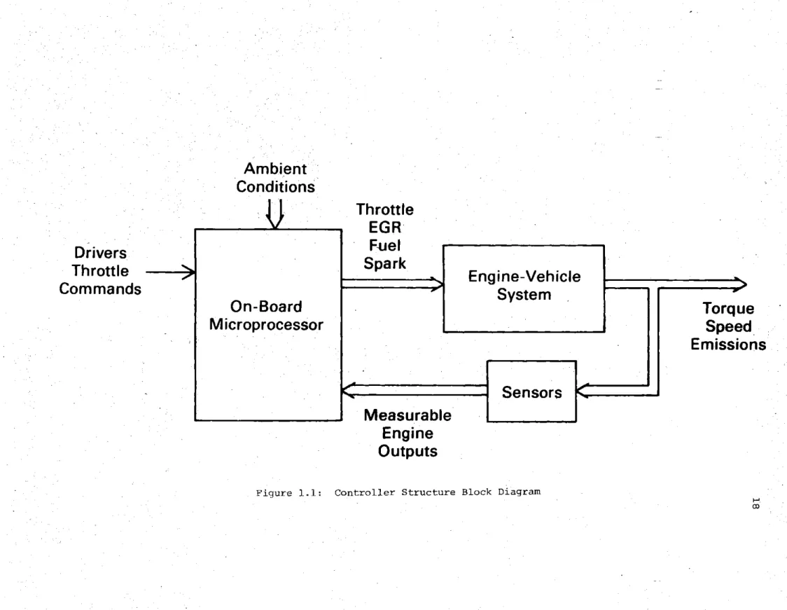
1.2 Controller Structure

It is only with the introduction of the, microprocessor that the concept of implementing elaborate LQG control policies has firmly

taken shape. Discrete state reconstructors and feedback gains are easily realized within the numerical capabilities of even simple microcomputer systems. In fact, within the next few years many production automobiles may already have an on-board computer system (used for other functions) which will be capable of implementing these LQG control algorithms.

The central idea is pictured in Figure 1.1. The microcomputer sys-tem is being used to control engine inputs in response to the driver' s requested throttle command. Notice that this "drive-by-wire" approach

(after the aerospace "fly-by-wire" control jargon) is fundamentally different than the nominal controller in that the driver has no direct

Drivers.

Throttle

Commands

Ambient

Conditions

Throttle

EGR

Fuel

Spark.

Sensors

Measurable

Engine

Outputs

Torque

Speed

Emissions

Figure 1.1: Controller Structure Block Diagram

OD

On-Board

Microprocessor

Engine-Vehicle

System

op-the nominal controller had a direct mechanical cable link to op-the throttle blades from the accelerator pedal. In this LQG scheme the control system exercises complete control over all four engine inputs and can dynamically coordinate them to achieve the desired transient response.

It should be noted that in practice the hardware used to implement this control would most likely be arranged in some fail-safe type of strategy, such as adding or subtracting control perturbations around nominally controlled mechanical connections so a microprocessor failure would not incapacitate the vehicle or result in a catastrophic system failure. These implementation details are best addressed at a later stage of the research, e.g. after multiple controllers have been tested, and will be omitted in the ensuing discussions.

For the purpose of this work the nominal control scheme is assumed to be implemented in the microprocessor along with the LQG controller. In order to achieve the steady state nominal control values discrete integrators will be appended to the inputs on the LQG controller so that the washout effect is achieved, i.e. no steady state LQG control action

(see Stein and Sandell [19]).

As with all microcomputer systems only discrete control algorithms

can be implemented. In this research the original continuous time

engine-vehicle model will be discretized and a discrete LQG problem will be solved from the start. The discrete sampling rate was selected as

aliasing on analog to digital conversion and adequately control the engine inputs while permitting enough time to allow for the numerical computations required of the control algorithm. It is straightforward to select a different rate, if desired, for the controller design.

1.3 Thesis Outline

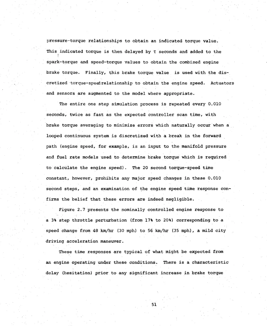
Immediately following this outline will be a brief summary of the major results of this research. Chapter II will present, in moderate detail, the development of the linear model used for the controller design; The physical bases for the model development will be stressed while the tedious numerical details and specific state space realization will be relegated to various appendices. Nominally controlled nonlinear Monte Carlo simulation results are presented which demonstrate a

noticeable torque hesitation and large air/fuel ratio deviations from stoichiometry in response to a step throttle command.

Chapter III presents the discrete LQG control algorithm design. The internal controller structure will be specified, the state recons-tructors designed, and the feedback gain selected to improve the transient

step response performance described in the nominal simulations in Chapter II. Again a complete set of nonlinear simulations is included to

demonstrate the improvements due to this LQG dynamic input coordination. Chapter IV presents a robustness of stability analysis for the previous chapters' model and control design. A, singular value apprQach

to robustness is outlined

and

appl~ed to this specific

engine

proWe

to afford at least some indication of the probable success, in terms of closed loop stability, of this control algorithm. This chapter hedges on the fringes of current research in the field of multivariable system robustness and some indication as to the drawbacks, advantages, and potentials of this singular value approach are included.

Chapter V briefly summarizes the major findings, conclusions, and

recommendations of this research. A selected bibliography, acknowledgements,

and complete appendices are included at the end of this work.

1.4 Major Contributions of this Research

A brief review of the major results of this research should help

focus attention on the important aspects while the reader pours over the necessary but tedious details of the next three chapters.

Basically there are three major points to be made. The first should come as no surprise to the seasoned veterans of the engine

control field, it is simply that dynamic engine modelling is a difficult task. _{The frequency range of the engine system, the nonlinearities, the} severe

cross

coupling, the inherent sampling nature of the four cycle internal combustion engine, and the limited output sensor dynamic capabilities all contribute to make this modelling step a most arduous assignment. _{The model presented in Chapter II represents the author's} "best" tractable dynamic linear approximation to the engine-vehicle system for the purposes of this LQG control project. The nonlinear Monte Carlo simulations are as accurate as practicable, using empirical

relationships for air-fuel-torque curves and matching physical data to

the linearized parameters.

_{These simulation results exhibit the type}

of system response one might expect, on intuitive grounds, from this

engine operating under these conditions.

This is, to some extent at

least, gratifying since the intent of the model was to capture the

es-sential engine system dynamics.

Chapter II should not be construed,

nor is it presented, as the final answer to the dynamic engine modelling

problem.

_{The work presented in this chapter should contribute, if even}

slightly, to this task while proving adequate for the controller design

and evaluation described in this thesis.

The second major result is that the simulations indicate again

(see Cassidy, Athans, and Lee [3]) that this LQ dynamic coordination of

all four inputs can lead to an improvement in the torque and air/fuel

ratio deviation from stoichiometry response to a driver's accelerator

commands.

_{This air/fuel ratio improvement should translate into improved}

tailpipe emissions since the conversion efficiency of the three way

catalyst is a strong function of this air/fuel ratio. The torque sag

seen in [3] and the torque hesitation seen here can be' eliminated by

this LQ control scheme.

Further, the LQ controller accomplishes the

kind of dynamic coordination, in response to 'the step commands tested,

that seems intuitively pleasing upon close examination. The throttle

blades are

opened

in a reasonably slow fashion, the fuel is increased

immediately then regulated for maintaining a stoichiometric air/fuel

ratio (approximately 14.6:1), and EGR and spark advance are decreased

and increased, respectively, to obtain the desired torque response.

The third major result concerns Chapter IV's robustness analysis.

Although the singular values of the LQG system are, at each frequency,

equal to or better than the "yardstick" nominal controller this does

not lead directly to the conclusion that the LQG -controller is as

robust as the nominal system.

This results from the fact that either

controller may be sensitive to a slightly larger, yet more plausible,

model perturbation.

At least at the high frequencies (4 Hz and above),

where the greatest modelling errors are expected, the LQG singular values

become large very rapidly, indicating a robust design in the face .of

high frequency

modelling errors.

The two basic pitfalls of a general multivariable singular value

robustness analysis were highlighted by this example.

They are that;

*

small singular values, indicative of a nearly unstable

design, can occur in modelling error directions which

can

be deemed (in

an

engineering sense) "implausible"

When this occurs the singular value analysis does not

yield much useful

information

because

modelling errors

in different directions, which might be deemed

"plausible", and having slightly larger singular values

might be destabilizing.

The singular value analysis

does not quantify this alternate yet plausible

results for this analysis are only in terms of the

forward path gain, or loop transfer gain,. pertur-bations, i.e. the plant-controller conbination. The item of interest is really destabilizing plant modelling error perturbations exclusive of the hand built and accurate controller. Translating the

forward path gain changes' resulting from this sin-gular value analysis into a meaningful class of destabilizing plant modelling errors is, in general a difficult task.

A complete collection of the detailed findings, conclusions, and recommendations of this work is included as Chapter V. Chapter II is now presented which describes the linear model development.

II. MODEL

"If you have $1,000 to spend on a control project spend at least $900 on model development"

an old control adage

2.1 Introduction

The ultimate success of any applications oriented control project hinges, to a great degree, upon the integrity of the underlying mathe-matical system model. _{A well developed and sophisticated control} algorithm designed around a plant model that poorly reflects reality will often lead to undesirable, and perhaps even dangerous, results. Unfortunately, there are no set rules governing just how accurate this plant model must be to assure project success. A judgement decision

must be made in light of the engineering tasks and control objectives at hand.

In a similar vein the type and scope of model chosen will depend upon the specific project objective under consideration. A model that

is too detailed and too complex runs the risk of obscuring important phenomena during the control algorithm synthesis. Conversely, an

overly simplified model may not capture the essential dynamics associated with the physical processes.

Perhaps no application highlights these inherent tradeoffs better than this engine control example. What is desired is a map,

G

which takes the vector of input functions, u, into the output functions, Yj as demonstrated in Figure 2.1. _{In state variable form this map becomes,}

26

ac

Throttle Position Command

Ec

EGR Value Position Command

Fc

Fuel Command

Sc

Spark Command

Tb

Brake Torque

N

Engine Speed

Pm

Manifold Pressure

Gp

Throttle Position

Ep

.EGR

Position

Tf

Filtered Torque

P

Filtered Manifold Pressure

X.= f(xu)

(2.

la)

Y g(x,u) (2. lb)

m

n

p

u eR

x

.R

yjER

As with all physical processes, and particularly for this engine example, the functions f and g are nonlinear. Further, the inclusion in exacting detail of the engine's distributed phenomena and the time delay associated with the induction process would necessitate the use of an infinite dimensional system. Even if the distributed phenomena are aggregated and the time delay approximated the system dimension can be prohibitively large since there is such a wide variety of events occuring in a broad frequency range. An accurate description of the "instantaneous" manifold pressure in an eight cylinder engine, for example, would require an analysis of the individual effects due to each of the eight intake values in addition to the more global effects of throttle angle and EGR pintle position

Continuing with this example; an average manifold pressure appears

to be a more meaningful quantity than this "instantaneous" pressure

since, in keeping with the stated control objectives of Chapter I, individual cylinder control is not an issue here. For this four cycle engine each cylinder inducts a new charge every other engine revolution, indicating that dynamic effects on the order of half engine speed and

above can

essentia'ly

be averaged ott in the model derivation.

This

effectively imposes an upper frequency limit on events of interest in the map,

0 < < N(2.2)

N

- engine

speed

- frequency of interest

Equation (2.2) is not a hard constraint, rather it represents *a guideline to be used when considering -which phenomena should be des-cribed by

0.

This in turn imposes restrictions upon the control

bandwidth and the required system robustness properties since

0

is - by

design - inaccurate in the half engine speed and above frequency range, an important fact that must not be overlooked in the controller

synthesis process.

This map,

0,

can be even further simplified since the control ob-jectives state that a linear quadratic controller is to be designed. The nonlinear functions, f and g, can be linearized about the nominal operating point,

X,

to obtain the perturbational equations,

x

= {xtu'} the set of nominal conditions x = x9 + 6x

u

=u +

Su

f(x*u*) 0

Y a=g(x,u2

6k

A6x +B6u

(2.

3a)

6y=

c6x

+ D6u (2.3b)

where

A

af

A

af

-

3x

u xD

ax

U XX

Again, the process of linearization, although a requirement for the development of an LQ controller, introduces even further excursions of the math model from the real engine. How large these errors are depends upon how nonlinear the original system is and upon the size of the perturbations around the nominal operating point. They will be

present, however, and a successful control design must be robust with respect to these linearization errors.

In addition to the bandwidth and linearization requirement it can also be important, where possible, to develop a model based upon first principle physical laws. This offers the distinct advantage o

affording opportunities for intuition into the control process and its limitations (a collection of force-acceleration data for one mass is not as valuable as a basic understanding of Newton's second law). In addition, the use of physical principles in the model development can save time and expense when a linearized model is desired about

different operating points.

The desired model, therefore, is alinear map, G, accurate for

frequencies from dc to half engine speed, based- as much as

possible-on physical principles.

The complete development of this model is covered

in detail by Lewis and Cassidy in [15].. Only an overview of the salient

points with sufficient depth to facilitate an understanding of the

processes involved and a grasp of the more complicated issues is

included here.

The engine separates naturally into six major categories,

1.

manifold pressure

2.

mass transport

3.

brake. torque

4.

engine speed

5.

actuators

6.

sensors

each of which will be individually discussed.

In addition, the concept

of a global nominal controller will be introduced and developed,

fol-lowed

by a brief discussion of the model's eigenstructure and time

response.

A short summiary will conclude this chapter.

2.2

Continuous Time

Model Derivation

2 2.1

Manifold Pressure

The manifold pressure dynamics, in the frequency range of interest,

are described using an ideal gas law analysis for a constant volume

cavity

-the

intake manifold.

Figure .2.2 illustrates the conceptual

Pm

m Out

o0 0 0

In.

Air

EGR

Fuel

qND

qND -Pm

mout m

2

₂

_RTm

process. Air enters the manifold through the throttle body, fuel is injected at the throttle body, and recirculated exhaust gas enters at the EGR value. The inlet air rate is, in general, a flow function of throttle angle, manifold and ambient pressure,

m

f ( P ,P

)

(2.4)

air

1

p

m

0

in

The fuel rate, due to the nature of the fuel injection logic used,

is a function of the fuel command voltage and engine speed,

mf f2(FcN) (2.5)

ful

2

c

In a manner entirely analogous to air flow the EGR rate is given

by a function of the EGR valve pintle position, manifold and exhaust

pressure,

m = f (E P P (2.6)

EGR 3 p m

e

The outlet mass flow rate is defined by the volumetric efficiency

as,

P-ND m m- = - -(2.7)

out

2

RT

m

where

n

1 the volumetric efficiency, Is given by Taylor and Taylor in

[43] as,

P P r- e/ m k-l T.=+

I(2.8)

k k3(r-1) 32 - - -

-T1 -

wide open throttle volumetric efficiency

k

- ratio

of

specific heats

r

- compression ratio

D

- engine displacement

T - manifold gasseous bulk temperature

R

- ideal gas constant

Differentiating the ideal gas law for the manifold mixture at constant bulk temperature results in,

RT

Mm

. (2.9)

m

V

in

out

V

=manifold

volume

m

Finally, substituting (2 .4)-(2.8) in (2.9) and linearizing about the nominal operating point yields the governing differential equation

for perturbed manifold pressure,

=P I

[(k-1).(r-l)

+

r-C'JND

m 2(r-l)kV m

m

TD{[(k-1)

(r-1)+r]P

-

P

m

6N

2k(r-l)V

m

RT + -

6

i.

+

666

+

6h

2.'10)

V air fuel EGR

S

fraction of fuel in "ideal gas" form

C1 e

Actual frequency and time domain experiments have verified the

predicted first order behavior, while the experimental pole position

and gain values are generally within 10% of those predicted by

equation (2.10).

2.2.2 Mass Transport

The air flow transport dynamics are given by the manifold pressure

equation (2.10). The mass flow at the cylinders was given by equation

(2.7) and represent the sum of the air flow, EGR and fuel flow resulting

in,

T)DP

ND

6P

+

m

6N

-6m -

(2.11)

air 2RT

m

2RT fuel EGR

m M

cylinders

cyl

cyl

-XyX

which is a deterministic equation in the fuel and EGR flows at the

cylinders and the manifold pressure.

The fuel and EGR transport dynamics are more complicated. Tanaka and Durbin in [16] present experimental data and a physical analysis of the fuel evaporation to describe the manifold transport dynamics for fuel perturbations. Research is currently in progress to extend their

work

to

include the convective and diffusive effects of non-liquid fuel transporqt and EGR. Preliminary experimental data tends to support that presented in [16] as a first approximation however, and their first order dynamic fuel model will be used. In the Laplace transform variable, s,

a

6(s)

_fuel =

(s)

(212)

s+ct

fuel

cylinders inlet

where the time constant,

1/a

in some sense increases 4th a charac-teristic manifold length and decreases with liquid fuel film velocity,

kz

1

o

- (2.13)

f

k

- constant

- characteristic manifold length

Vf

-

fuel velocity

(liquid

film)

The EGR transport dynamics are complicated by the extreme tem-perature variation between the recirculated exhaust gas and the bulk manifold flow as well as the pressure resonances between the exhaust and intake manifold cavities. Coupling between perturbations in the high temperature EGR flow and the rate of evaporation of liquid fuel necessitates an even more detailed analysis, research which - at the time of this writing -'is currently in progress. For the purposes of

this linear quadratic control design study the empirical data will be used which suggests that these dynamics can best be approximated by a third order linear system.

2.2.3 Brake Torquae

The engine torque analysis presented here closely parallels that given by Taylor in [43] and begins with the definition of engine

efficiency,

n

=

out

(2.14)

e P.

in

P - power out of the engine system out

P. - power in to the engine system in

Assuming that all energy transfers of interest across the system boundary are associated inward with the fuel flow and outward with the output shaft power then (2.14) can be written as,

TbN

S

k b(2.15)

e

fuel

higher heating value of the fuel

T

- engine brake torque

b

N

- engine speed

k -

conversion constant

Rearranging (2.15) and absorbing the constant into one term yields,

k Tj

e fue

T =ful(2.16)

b

N

The efficiency variable in this equation is, in general, a function of the dilution factor, manifold pressure, spark advance, and engine speed,

-

=f

₄

(DF, PS,

N)

(2.17)

e 4 m

+xh

air

EGR

DF m fuel cylinders

Equation (2.16) and (2.17) can be linearized about the operating point to obtain the steady state gains,

6T

=k

dxh.

+k

6h

+ k

6+k

+ k

6P

b

11 air

12

EGR

13

fuel

14 m

SS

(2.18)

k

6S

+

k

6N

15

16

The variation of steady state brake torque with perturbations in EGR rate, manifold pressure, spark advance, and engine speed is fairly linear at the operating point of interest. In that respect, therefore,

(2.18) is a good approximation to reality. Around this stoichiometric point, however, torque is a highly nonlinear function of air and fuel flows, as the experimental data presented in Figure 2.3 illustrates.

Torque -14 -- O

a2

a

Nominal

K

1

Tb

MrAir

0

m

Constant

Fuel

b

Figure 2.3: Air-Fuel -Torque Curves

Nominal

K1

m Fuel

m Ar

=

Constant

Air

C 38

Torque

-S?

al1

Tb

$

For this linear model the curves can be linearized about the nominal

operating point to obtain the nominal gains.

For simulation studies

the actual nonlinear curves must be used to obtain reasonably accurate

results. A successful control design must first attempt to maintain

the stoichiometric operating conditions (thus preventing large

deviations in the values of k

and kl) and second be robust to the

11 13

remaining persistent air-torque and fuel-torque gain changes.

The dynamics associated with the brake torque equation are due to

the inherent sampling nature of a four cycle engine.

An instantaneous

perturbation in fuel rate at the cylinders, for example, must first be

inducted, compressed, and then ignited before any perceptible change

in brake torque will occur.

This introduces a time delay in equation

(2.18) for the air, EGR, fuel, and pressure terms (spark and speed

effects on torque are assumed to be instantaneous),,

ST (t)=

k

&h

(t-T)

+ k

Si

(t-T) + k

Sn

(t-T)

b

11

air

12

EGR

13

fuel

(2.19)

+

k

₄

6P

(t-T)

+

k

6S(t)

+

k

6N(t)

14

m

15

16

where the limits on the time delay,

7,

are

60

60

T

<

(

2N

N

The

lower

limit

corresponds

to a perturbation just at the end of an

beginning of an intake stroke. Of course, for a multicylinder engine

these regions are not sharply defined, and a good approximation to this sampling phenomenon is an averaged time delay,

3*60

_V60

_(2.21)

T

= 4N

2.2.4 Engine

Speed-The speed dynamics chosen here are intended to reflect the

behavior of an engine in a car equipped with an automatic transmission. The two important physical factors which map the perturbed engine brake

torque,

6Tb

to a perturbed engine speed,

6N,

for this case are the reflected vehicle inertia and the torque converter. Kotwicki in [14] presents a physical argument and experimental data to suggest that these factors can be dynamically represented as a second order linear system with one pole representing the vehicle inertia (approximately a 20 second time constant) and a pole-zero combination to handle

slippage in the torque converter, in the Laplace transform variable s

6N(s)

k(s+z)

6T

(s)

(2.22)

(s+p1) (s+p2) b

2.2.5 ActuatQrs

The actuators modelled are those typically found in a dynamometer-engine test cell environment. The throttle actuator is assumed to be of the dc motor type and is modelled as a second order linear system.

The EGR actuator is a pulse width modulated vacuum type with a position control loop and is also modelled as a second order linear system. The injector logic for the throttle body fuel injection system

schedules the width of fuel pulses (four every engine revolution) with a fuel command voltage. The response of the fuel rate at the injectors to a change in this command voltage is instantaneous (in the frequency range of interest) and no dynamics are assumed here. Similarly, the

spark responds instantaneously in this time frame to perturbed spark commands.

2.2.6

Sensors

The brake torque sensor is of the strain gauge type and has a cutoff frequency in the 2 kHz region. In practice this results in a torque signal which reflects each cylinder firing and some filtering must be done to obtain an average torque signal for the half engine speed and below frequency range. In addition, this filtering is

required to prevent aliasing of the sampled signal. A third order filter was found acceptable for these purposes.

The engine speed signal is obtained from a tachometer coupled to the output shaft. Its associated electrical poles are assumed to be much higher than the half engine speed of interest and no dynamics are included here.

The manifold pressure transducer is of the semiconductor type and reacts to every opening intake value. Just as in the case of the torque

sensor this signal must be filtered and a second

order

filter model was employed for this purpose.

The throttle angle and EGR pintle position feedback signals are obtained from linear potentiometers and no dynamics are used.

2.2.7

Block Diagram

A block diagram for the engine mode, complete with actuators and sensors, is included as Figure 2.4. Numerical values for the constants are included in Appendix B. Appendix A contains the

derivation of the state equations used to develop the system matrices, [A, B, C, D] referenced in the remainder of this report, Finally, for completeness, the numerical values for these matrices are presented in Appendix C.

The engine model, using a second order Pade approximant for the

engine time delay, is a nine state model.

The actuators add four

states while the sensors add five for a total system dimension of 18.

2.3 Discrete Time Model

Since the final implementation for a control algorithm of this

type is envisioned as a microprocessor based system a discrete time

control law will be developed.

Two approaches are possible. First,

Pressure DynamicE K2

2-c

9

K1 + 2+mEnG s2f2tg110 2 f P + + - +S+ s2 1 +09 + Throttle Actuator KK68

SEC

2 a - 2 EGI S2+20 12al s3KE -E0 +2s 5)-S2+2C1a .7a7 K1j EGR Actuator. I -*--*-I 2 sU13 Pressure Filter 0 a - 0 L 0 mFuel.

EGR Transport Dyr

8

F K9

Fc +a6

K3 K

s+ 6

K4 _{Fuel Transport Dynamics}

8

Sc _ K17 R Air K16 K11 ++ STi -- s +, K1.0 3 4 (s+d2) 02 K13 T '1e y

orque-Speed

Dynamics - - .14Tt

UP

1

8Pm

- 8N I A a a -A.Mon I I K18 namics

.BTi

a continuous time control law can be designed, then discretized for implementation. Second, the original continuous time plant model can be discretized and a discrete time controller designed from the start. There appears to be no hard and fast rule governing which is best for any specific application, and the later approach is adopted here.

The discrete model derivation follows. Using a standard procedure for matching the continuous time sampling interval step response to the piecewise constant inputs from a zero order hold digital to analog device the discrete model becomes,

6x(k+l)

= A6x(k) + B6u(k) (2.23a)

6y(k)

= C6x(k) + D6u(k) (2.23b)

where, from the variation of constants formula for this linear time invariant system,

AA A(A(A-T)

A=e- ;

B=]e-

BdT

0

Both the continuous and discrete systems will be referenced in the ensuing work and the circumflex (A) distinction for the discrete time

dynamic and input matrices will be carried throughout.

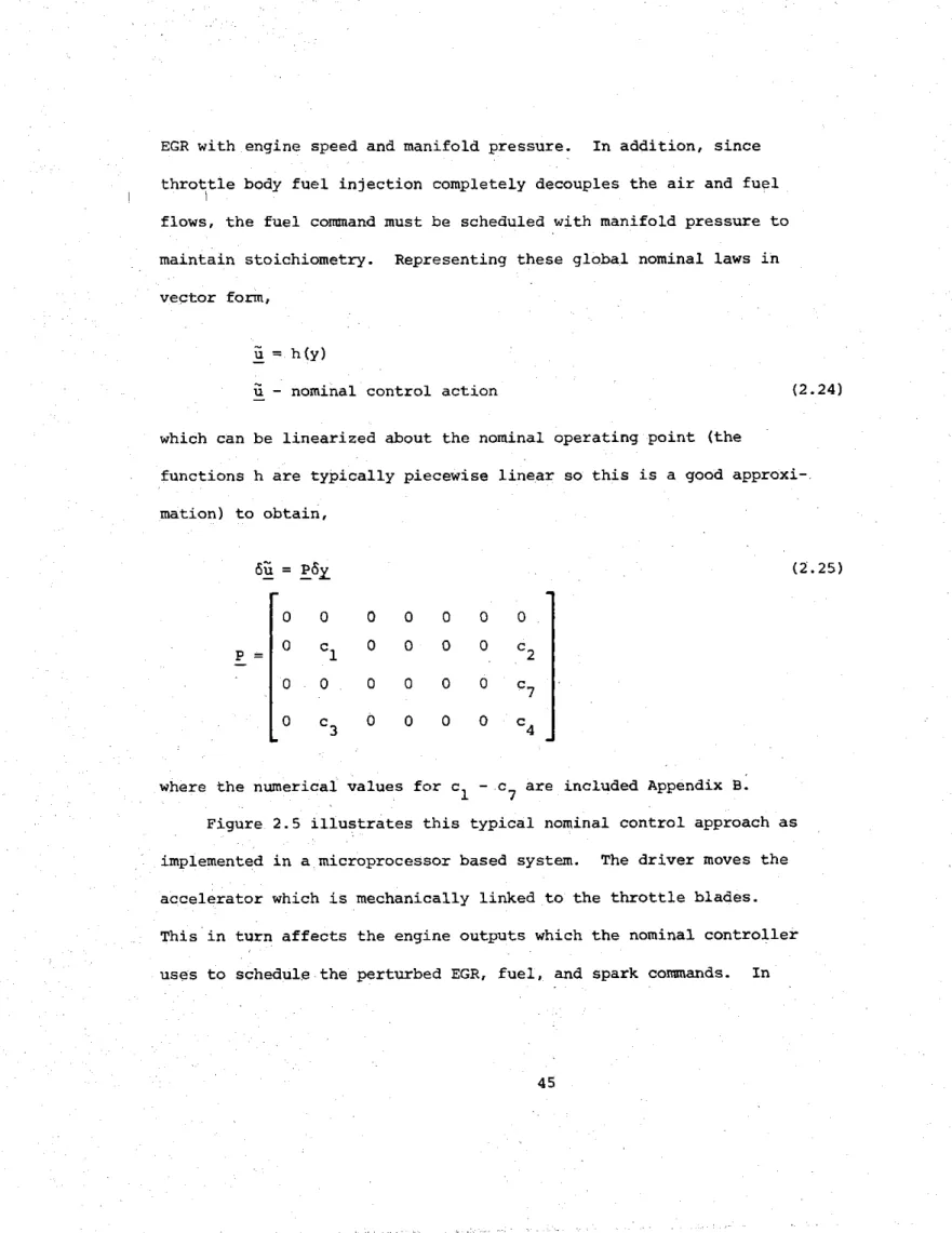
2.4 Nominal Controls

Automotive engines in current production include some type of global nominal control law (mechanically implemented in the past, often microprocessor based today) which schedules spark advance and

EGR with engine speed and manifold pressure. In addition, since throttle body fuel injection completely decouples the air and fuel flows, the fuel command must be scheduled with manifold pressure to maintain stoichiometry. Representing these global nominal laws in

vector form,

u

=h(y)

-

nominal control action (2.24)

which can be linearized about the nominal operating point (the

functions h are typically piecewise linear so this is a good approxi-mation) to obtain,

6

=

P y

(2.25)

0

0

0

0

0

0

0

0

c

1

0

0

0

0

c

o

0

0

0

0

0

c

7

0

c

3

0

0

0

0

C

3 4

where the numerical values for c -

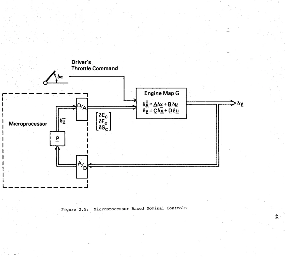
c

7 are included Appendix B.

Figure 2.5 illustrates this typical nominal control approach as implemented in a microprocessor based system. The driver moves the accelerator which is mechanically linked to the throttle blades. This in turn affects the engine outputs which the nominal controller uses to schedule the perturbed EGR, fuel, and spark commands. In

Driver's

Throttle Command

Engine Map G

1Q

__

xAbx+Bbu

8y = Cox+ Dou 8Ec

Microprocessor

C

P

IA

I

YD

L4

Figure 2.5: Microprocessor Based

Nominal Controls

4 0~

practice other systems, such as a zirconium sensor based air/fuel ratio control, may be present but will not be considered in this

work. The nominal controller defined In equation (2.25) and illustrated

in Figure 2.5 represents the baseline control scheme against which the

LQ design will be compared from both a time response and robustness

perspective.

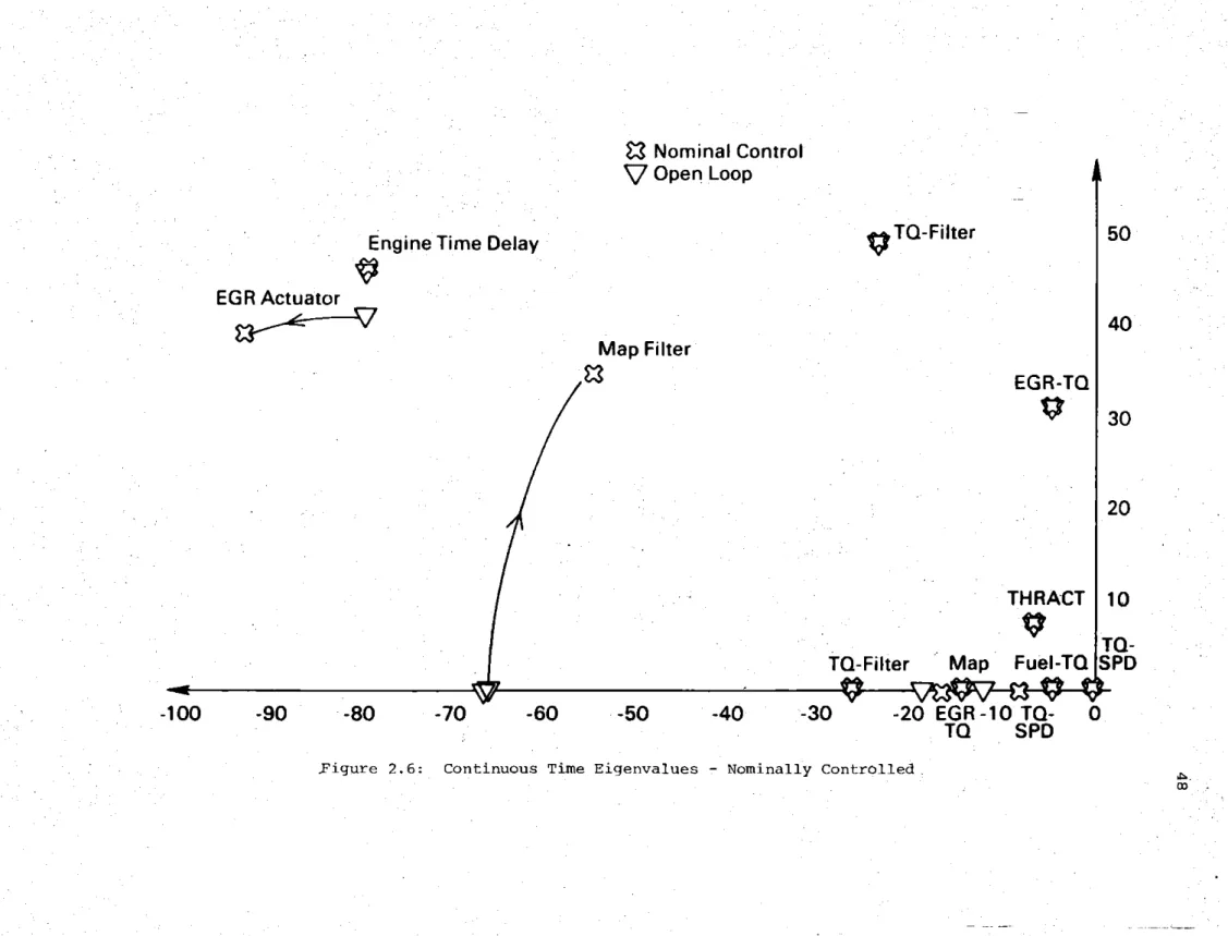
2.5 Eigenstructure

The high system dimension (18 states) in this example precludes all but the most cursory eigenstructure analysis. A polar plot of the

eigenvalues for both the original uncontrolled model and the nominally controlled model is included as Figure 2.6 where, for the uncontrolled plant the eigenvalues

A,

are defined by,

x

Ax(2.26)

and,

for nominal control,

(A + 13 p C)x,= X (2.27)

These eigenvalues range in speed from the slow

(

20 second time

constant) torque-speed pole representing the vehicle inertia to the 14.6 Hz Pade approximant used to represent the engine time delay.

The

model

is, by design, both

completely controllable and

com-pletely observable as confirmed by a standard eigenvector

analysis

$2

Nominal Control

V

Open Loop

.vTQ-Filter

Engine Time Delay

EGR Actuator

Map Filter

EGR-TQ

THRACT

-80

-70

-60

-50

-40-

-3C

50

40

30

20

10

Ta-Filter

TPD

-20 EGR-10 TQ-

0.

TQ

SPD

Figure

2.6: Continuous Time Eigenvalues - Nominally Controlled,

03

(see Stein and Sandell [19]). Some interesting system theoretic results for the nominally controlled system are,

all 18 modes are controllable from the throttle input and (of course) the throttle actuator modes are only controllable from the throttle

input.-* The three torque filter modes are observable only in the filtered torque signal. This is not surprising since that signal is the only one not fed back by the nominal controller and not coupled in the block diagram. All 18 modes are observable in the filtered

torque signal.

0 With the exception of the above mentioned torque filter modes the remaining 15 modes are equally observable in the torque or speed

signals.-* The manifold pressure signal may also be used to observe these 15 modes, with the exception

of the two modes associated with the engine

time delay which are only. weakly observable

in the pressure signal.

The above statements result from inspection ot the controllability and observability matrices defined here as,

Controllability Matrix = Y B (2.28)

where Y and X are the suitably normalized left and right eigenvectors given by, Y(A + B P C) =

A

Y (2.30)

(A

+

B p C)X

=

X

A

(2.31) Y

X

I (2.32)

A

diag(X

₁

N

₂

f... ,X )

1

2

18

Equations (2.28) and (2.29) are subject to scaling, a fact which must

be considered when interpreting the results.

2.6 Simulations

Since one of the objectives is to improve the torque and air fuel

ratio transient response to step throttle changes it seems appropriate

at this time to briefly discuss the computer simulation technique used

in this analysis.

Basically the approach has been to discretize the differential

equations presented in section 2.2 to propagate the perturbed inputs,

throttle, EGR, fuel, and spark commands, into the manifold pressure and

the air rate, fuel rate, and EGR rate at the cylinders.

The cylinder

rates are then used with the nonlinear air-fuel-torque relationships

pictured in Figure 2.3 and linearized EGR-torque and manifold