Publisher’s version / Version de l'éditeur:
International Polymer Processing, 27, 1, pp. 111-120, 2012-01-01
READ THESE TERMS AND CONDITIONS CAREFULLY BEFORE USING THIS WEBSITE. https://nrc-publications.canada.ca/eng/copyright
Vous avez des questions? Nous pouvons vous aider. Pour communiquer directement avec un auteur, consultez la
première page de la revue dans laquelle son article a été publié afin de trouver ses coordonnées. Si vous n’arrivez pas à les repérer, communiquez avec nous à PublicationsArchive-ArchivesPublications@nrc-cnrc.gc.ca.
Questions? Contact the NRC Publications Archive team at
PublicationsArchive-ArchivesPublications@nrc-cnrc.gc.ca. If you wish to email the authors directly, please see the first page of the publication for their contact information.
NRC Publications Archive
Archives des publications du CNRC
This publication could be one of several versions: author’s original, accepted manuscript or the publisher’s version. / La version de cette publication peut être l’une des suivantes : la version prépublication de l’auteur, la version acceptée du manuscrit ou la version de l’éditeur.
For the publisher’s version, please access the DOI link below./ Pour consulter la version de l’éditeur, utilisez le lien DOI ci-dessous.
https://doi.org/10.3139/217.2450
Access and use of this website and the material on it are subject to the Terms and Conditions set forth at Three dimensional numerical study of the mixing behavior of twin-screw elements
Ilinca, F.; Hétu, J.-F.
https://publications-cnrc.canada.ca/fra/droits
L’accès à ce site Web et l’utilisation de son contenu sont assujettis aux conditions présentées dans le site LISEZ CES CONDITIONS ATTENTIVEMENT AVANT D’UTILISER CE SITE WEB.
NRC Publications Record / Notice d'Archives des publications de CNRC:
https://nrc-publications.canada.ca/eng/view/object/?id=366569c5-3b81-4b69-88a8-abcded11798d https://publications-cnrc.canada.ca/fra/voir/objet/?id=366569c5-3b81-4b69-88a8-abcded11798d
1
Three-dimensional numerical study of the mixing behaviour of
twin-screw elements
Florin Ilinca
Jean-François Hétu
Industrial Materials Institute, National Research Council,
75, de Mortagne, Boucherville, Québec, Canada, J4B 6Y4
Email: florin.ilinca@cnrc-nrc.gc.ca
Phone: (450) 641-5072
FAX: (450) 641-5106
June 2, 2011
A paper submitted for publication in the International Polymer Processing Journal All correspondence to be sent to: Dr. F. Ilinca.
2
Three-dimensional numerical study of the mixing behaviour of
twin-screw elements
Florin Ilinca and Jean-François Hétu
Industrial Materials Institute, National Research Council,
75, de Mortagne, Boucherville, Québec, Canada, J4B 6Y4
Abstract
In this work the numerical modeling of the flow inside co-rotating twin-screw extruders is performed and solutions are analyzed to determine the mixing behavior of two screw elements: conveying and mixing elements. The flow around intermeshing screws is computed using an immersed boundary finite element method capable of dealing with complex moving solid boundaries. The flow is considered isothermal and the material behaves as a generalized non-Newtonian fluid. Because the viscosity depends on the shear rate, solutions will be shown for various rotation velocities of the screw. The 3D solutions are then analyzed in order to determine various parameters characterizing the flow mixing such as the residence time and the linear stretch. Residence time distribution inside the twin-screw extruder is first computed by using a particle tracking algorithm based on a fourth order Runge-Kutta method. A large number of particles are tracked inside the extruder and the resulting particle data is used to determine the distribution of the residence time and of the linear stretch. The spatial distribution of the residence time is also computed by solving a transport equation tracking the injection time of the polymer melt. The methodology shows important differences in the mixing behavior of the screw elements considered.
3
1. INTRODUCTION
Screw extruders are widely used in the plastic industry to plasticize polymers, i.e. to increase their temperature up to a desired value for injection molding applications, and to achieve a desired degree of mixing by distributing and dispersing the polymers. Twin screw extruders are commonly used and they are classified by the rotation direction of each screw (co-rotating and counter-rotating), the degree of intermeshing and the type of screw elements. For co-rotating screw extruders three types of elements are widely used: the full flight screw, the kneading blocks and the screw mixing element consisting of a standard screw profile with slots cut across the flight tip to increase the flow leakage.
Efficient application of twin-screw extruders requires characterization of the mixing behavior of various screw elements a task that can be tackled efficiently by numerical simulation. First attempts to simulate twin screw extruders addressed only a 2D analogy of the flow (Speur et al. 1987, Kajiwara et al. 1996, Bravo et al. 2000). Bertrand et al. (2003) presented a fictitious
domain method based on a mesh refinement technique overlapping a single reference mesh. The mesh is locally adapted to enrich the discretization in small gaps and applications are shown for 2D flow simulation in twin-screw extruders. Kajiwara et al. (1996) developed a 3D numerical technique to simulate fluid flow in the case of full flight conveying screw elements. Their simulations were however restricted to one section of the analysis domain, located in the nip region, and relied upon periodic boundary conditions. Cheng and Manas-Zloczower (1997, 1998) and Yao and Manas-Zloczower (1998) reported 3D numerical studies of co-rotating twin screw extruders using the commercial software FIDAP. Their approach was based on selecting a number of sequential geometries representing various positions of the screws in order to represent a complete cycle and then computing steady state solutions for each of them. The dispersive
4 mixing efficiency of the flow field was assessed in terms of its elongational flow components and magnitude of shear stresses. Zhang et al. (2009) uses a mesh superposition technique to solve intermeshing twin-screw extruders without remeshing. The procedure, incorporated into the Polyflow software, generates finite element meshes for the flow domain and each screw element, respectively, which are then superimposed. The position of each screw is then updated at each time step. In their study, particle tracking is used to generate the distribution of the residence time inside kneading disks elements. The mixing performance and efficiency is also determined using the framework developed by Ottino et al. (1981). Three-dimensional solutions of the steady state flow and energy equations inside twin-screw extruders are reported by Ishikawa et al. (2000). The Stokes equations describing the polymer flow are solved separately for each flow domain corresponding to successive positions of the screw. The same approach is applied to the energy equation by including the convective term but neglecting the transient effects. One drawback of such an approach is that while the polymer melt may reach a quasi-steady state (or periodic variation), the heat transfer should take into account the coupling between the convective transport and the actual change in the flow domain. Therefore, the steady state solution of the energy equation should only be seen as an approximation of the global heat balance inside the screw extruder. Kalyon and Malik (2005, 2007) used the same steady-state framework to describe the flow and heat transfer of generalized Newtonian fluids inside co-rotating and counter-rotating twin screw extruders. Their studies investigate the pressure distribution inside combinations of multiple screw elements and inside screw-die configurations. Lawal and Kalyon (1995) used a particle tracking approach to analyze the mixing occurring in single and co-rotating twin screw extruders with kneading discs elements.
The main hurdle when modeling the flow inside twin-screw extruders is the continuous change in the computational domain determined by the rotation of the screws. On the other hand, a
5 simplifying behaviour is that inertia is negligible for molten polymers. This results in the flow solutions depending only on the conditions at the current time step. At this point, almost all numerical simulations of 3D twin-screw extruders were performed using a sequence of steady-state solutions on different meshes representing the successive positions of the screws. Such an approach is not complicated in terms of 3D flow solution, but instead forces the use of more complicated solution techniques when flow solutions should be transferred from one time step to the next as is the case for particle tracking algorithms. Moreover, such approaches are not appropriate if one need to solve the energy or other scalar transport equations for which the inertia cannot be neglected.
In the present work we use an immersed boundary (IB) method solving the equations on a mesh that do not represent the screw surfaces. IB techniques rely on using simple grids on domains of simple shapes with the discretization being performed on a single domain enclosing both fluid and solid regions. These methods trade the geometrical complexity of the domain of interest for the simplicity of easy to create geometries using relatively uniform meshes. This necessitates however abandoning a simple implementation of boundary conditions for a more complex one. In most IB methods, boundary conditions on immersed surfaces are handled either accurately by using dynamic data structures to add/remove grid points as needed or in an approximate way by imposing the boundary conditions to the grid point closest to the surface or through least-squares. Our recently proposed approach (Ilinca and Hétu, 2011) achieves the level of accuracy of cut cell dynamic node addition techniques with none of their drawbacks (increased CPU time and costly dynamic data structures). This approach was extended to moving fluid/solid interfaces (Ilinca and Hétu, 2010a) and to single and twin-screw extruders (Ilinca and Hétu, 2010b). For problems involving convective transport, the proposed IB method was shown to predict adequately the flow structures produced by the continuous repositioning of the solid
6 surfaces. The use of a single mesh makes then easier the solution of transport phenomena as those encountered for particle tracking and residence time computations.
The paper is organized as follows. First the model problem and the associated finite element formulation are presented. The IB formulation and the procedure to impose the boundary conditions on moving solid surfaces are discussed briefly. Section 3 discusses the methodology to compute the distribution of the residence time and the linear stretch. Section 4 illustrates the application of the IB method to 3-D co-rotating twin-screw extruders and the analysis of the mixing behavior of conveying and mixing elements. The mixing behavior of twin-screw elements is quantified by the analysis of the flow based on parameters such as the residence time and the linear stretch. The paper ends with conclusions.
2. NUMERICAL MODELING OF THE FLOW
2.1. Flow equations
The flow of melted polymers is described by the incompressible Stokes equations
0 p ( u uT) , (1) 0,
u (2)
where u is the velocity, p is the pressure and is the viscosity. The material is considered as behaving as a generalized Newtonian fluid with the viscosity described by the Cross model:
1 ( ) 1 / * r n r (3)where model constants take on values corresponding to polystyrene at 200˚ω (Ilinca and Hétu, 2001): n0.26, 4
* 2.5 10 Pa,
3
3.841 10 .
r Pa s
The viscosity dependence upon the shear rate is shown in Figure 1.
7
Figure 1: Viscosity of polystyrene at 200°C.
The interface between the fluid and solid regions is defined using a level-set function ψ which is defined as a signed distance function from the immersed interface:
( , ), in the fluid region, ( ) 0, on the fluid/solid interface,
( , ), in the solid region,
i i d d x x x x x x x x (4)
where d(x,xi) is the distance between the point P(x) and the fluid/solid interface. Hence, points in
the fluid region will take on positive values of ψ, whereas ψ for points in the solid region will be negative.
2.2. Boundary conditions
The boundary conditions associated to the momentum-continuity equations are
( ), for , d D u U x x (5) ˆ ˆ ( T) ( ), for , t p u u n nt x x (6)
where ΓD is the portion of the fluid boundary where Dirichlet conditions are imposed, and t is the traction imposed on the remaining fluid boundary. Dirichlet boundary conditions are also
8 imposed at the interface between fluid and solid regions. Because this interface is not represented by the finite element discretization, a special procedure is used to enforce velocity boundary conditions on this surface. This approach will be discussed in the Section 2.4.
2.3. The finite element formulation
In this work we discretize the momentum-continuity equations (1)-(2) using a GLS (Galerkin Least-Squares) method with linear continuous shape functions for both velocity and pressure. This leads to the following weak formulation:
t T d p d d
u u v
v
t v (7) 0 K K K qd p qd
u
(8)where v and q are continuous, piecewise linear test functions associated to the velocity and pressure equations. The stabilization parameter τ is computed as:
2 . 4 k K m h (9)
Here hK is the size of the element K and mk is a coefficient set to 1/3 for linear elements (Franca
et al., 1992). The GLS method contains additional stabilization terms which are integrated only on the element interiors. These terms deal with the velocity-pressure coupling so that equal-order interpolation results in a stable numerical scheme (Hughes et al., 1986; Franca et al., 1992). This makes it possible to use elements that do not satisfy the Babuška-Brezzi condition as is the case of the linear P1-P1 element (Hughes et al., 1986). GLS also stabilizes the resulting linear systems, making them tractable by robust iterative solvers. This last advantage is very important for large scale applications. This finite element method was successfully applied by the authors to various injection molding applications (Ilinca and Hétu 2001, 2002, 2003).
9
2.4. The immersed boundary method
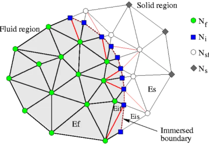
The computational domain contains the entire volume that at any time it may be occupied by the polymer melt. This means that part of the domain falls inside moving mechanical parts which are considered as a solid region. Because the intermeshing screws rotate, the interface between solid and fluid regions moves and parts of the computational domain switch from fluid to solid or from solid to fluid. At any time step the mesh is therefore intersected by the fluid/solid interface at points located along element edges and we consider those points as additional degrees of freedom in the finite element formulation. A special treatment is then applied to solid region and interface degrees of freedom. Figure 2 illustrates a simple case where the mesh is shown by the continuous lines, the interface is indicated by the discontinuous line and the additional interface nodes are indicated by the square symbols. The technique was implemented for 3-D meshes but for the ease of the presentation only a 2-D case is shown in Figure 2.
Figure 2: Decomposition of interface elements for IB method.
The fluid/solid interface is defined by the level-set function and therefore the additional interface nodes are easily determined as being those for which =0. Moreover, because the level-set function is interpolated using linear shape functions, the intersection between the interface
10 and a tetrahedral element is a plane, either a triangle or a quadrilateral. Elements cut by the interface are therefore decomposed into sub-elements which are either entirely in the fluid or entirely in the solid region. The additional degrees of freedom associated to the nodes on the interface would normally determine a modification of the global matrix resulting from the finite element equations. In such a case, the implementation is more challenging and would result in an increase in computational cost inherent to dynamic data structures and renumbering. The present IB approach does not need the explicit addition of the degrees of freedom associated to those nodes. The degrees of freedom associated to the interface nodes are eliminated at the element level by using the Dirichlet boundary conditions for the velocity and by static condensation for the pressure. Hence, the pressure interpolation is taken continuous except for the element faces cut by the interface where it is discontinuous. The procedure results in the local enrichment of the velocity and pressure discretizations. For more details regarding the implementation of the IB method the reader may consult (Ilinca and Hétu, 2011, 2010a).
3. STUDY OF THE MIXING BEHAVIOR
The mixing behavior of twin-screw elements is quantified by the analysis of the flow based on parameters such as the residence time and the linear stretch. Those parameters and the way they are computed are detailed in this section.
3.1. Residence time
We propose two different methods to analyze the residence time (RT) of the polymer inside the region covered by screw elements. The first approach is based on the continuous injection of virtual particles on various locations at the entry of the screw element under investigation (Zhang, et al. 2009). It is assumed that these particles are massless, volumeless, and noninteracting with
11 each other. In other words the particles move at the same speed as that of the polymer and do not affect the flow. In the numerical simulation detailed in the next section the screw elements are located between x=0 and x=L with L being the screw element length with the polymer flowing in the positive direction of the x axis. Flow solutions are obtained at different time steps with a time increment of T/40 where T is the rotation period of the screw. The particles tracked for the RT computation are injected at x=0 with a uniform distribution in the y-z plane. A number of 440 particles are injected at each time step of a complete rotation for a total number of particles of 17,600. For each particle the RT is determined as the time to travel from the entry to the exit of the screw element (at x=L). The RT distribution is then determined by using the following relationship (Zhang, et al. 2009):
Number of particles with RT [ / 2, / 2] For / 2 / 2, ( )
Total number of particles
i i i i t t t t t t t t t E t (10)
The resulting RT distribution E(t) is normalized in the sense that
0 ( )d 1 t t E t t
(11)The second approach for estimating the RT distribution is able to provide a continuous response from which a spatial distribution of the RT can be recovered. Instead of tracking particles individually, in this case we consider a level-set method on which the tracking function φ measures the time passed inside the screw by the polymer. For this, we initialize φ to the current time at x=0 (entry of the screw element) and we solve the transport of the tracking function with the velocity of the polymer flow
0
t
12 At a given location, say the screw element exit x=L, and time t, the RT distribution is determined as RT , thus representing the difference between the present time and the time t
when the flow cell found at the respective location entered the screw element.
3.2. Length stretch
As for the residence time analysis, the stretch determined by the flow can be analyzed by using the particle tracking approach. The length stretch is defined as the rate of change of the distance between a pair of neighboring particles (Ottino, Ranz and Macosko 1981):
0
x x
(13)
where represents the magnitude of the vector formed by the initial location of the pair of x0
particles and measures the distance between the two particles at the current time t. The x
tracking of particles for estimating the length stretch is performed by following a large number of particles regrouped initially in clusters of very small dimensions. Following (Cheng and Manas-Zloczower 1998), for a system for which particles are initially gathered in l clusters with the jth cluster being formed by Nj particles, the length stretch distribution is computed as
1 , , 1 / 2 l j j j M t g t N N
(14)where M
,t is the total number of pairs with length stretch ranging from
/ 2
to
/ 2
at time t. As for the RT distribution, the length stretch distribution is normalized such as
0 g , dt 1
(15)13 Furthermore, the average length stretch can be obtained from the length stretch distribution as
0 , d t g t
(16)The average length stretch measures the capability of the mixing device to spread across the flow field particles initially located at very close locations.
As for the RT computation, the length stretch is a local measure depending on both the initial location of the pair of particles and on the initial time from which particles are tracked. Here we consider 250 clusters uniformly distributed in the plane y-z at x=0 and t=0, each cluster being formed by 8 particles placed on the corners of a cube of side length δ. A total of 7,000 pairs of particles are therefore followed for length stretch computations.
4. NUMERICAL APPLICATIONS
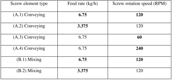
In this section the IB solution algorithm is used to solve the flow inside twin-screw extruders. The IB finite element method was validated against solutions on body conforming meshes in a previous work (Ilinca and Hétu 2010b) and therefore is not revisited here. Two different configurations are studied containing either conveying or mixing elements and the mixing behavior of each of them is analyzed. The extruder configuration and flow parameters considered are summarized in Table 1. Reference conditions are A.1 and B.1 for the conveying and mixing elements respectively and then, for each additional configuration, the parameter that changes is shown with bold characters. We choose here to study separately different types of screw elements in order to assess their mixing behavior, a task that cannot be done if we consider a combination of various screw elements.
14 Screw element type Feed rate (kg/h) Screw rotation speed (RPM)
(A.1) Conveying 6.75 120 (A.2) Conveying 3.375 120 (A.3) Conveying 6.75 60 (A.4) Conveying 6.75 240 (B.1) Mixing 6.75 120 (B.2) Mixing 3.375 120
Table 1. Screw configuration and flow parameters
Figure 3 shows the computational domain for the two screw elements considered, with the fluid region being shown in transparent gray. A cross-section of the grid at x = L/2 is also shown. The conveying element is a right-handed full flight screw, whereas the mixing screw element is a similar right-handed screw with left-handed slots. The flight length of the slots is twice that of the base element. The mesh has a total of 595,455 nodes and 2,870,400 tetrahedral elements. Both screws rotate anti-clockwise at angular speed and the polymer enters the domain in the positive
x direction. The geometry of the screws is indicated in a cross section in Figure 4. The barrel
radius is R=10.15mm, while the screw dimensions are R1=10mm, R2=6.25mm and d=3mm. The distance between the centers of rotation of the two screws is Δz=8.2mm and the screw element length is L=20mm (one complete screw flight). The computational domain contains one region at the entry of the flow and another at the exit where is no screw and the rod has a radius equal to the smallest radius of the screw elements (R2). Both screws rotate anti-clockwise when looking in the positive direction of the x axis as shown in Figure 4.
15 (a) Conveying element (b) Mixing element
Figure 3: Computational domain for the two screw elements.
Figure 4: Screw geometry for conveying element.
4.1. Flow solution
We present here the influence of the screw type, feed rate and screw rotation speed on the distribution of the velocity and pressure inside the polymer melt. Note that the inlet flow rate is much smaller when compared with the screw rotation speed and therefore has little influence on
16 the velocity distribution (case A.2 compared to A.1 and case B.2 compared to B.1). It will however affect the residence time inside the screw which will be discussed in the next section.
(a) Conveying element (b) Mixing element
(c) Effect of rotation speed (A.1, A.3, A.4) (d) Effect of screw element type (A.1, B.1)
Figure 5: Velocity v profile at x=L/2 and y=0.
Figure 5 shows the y-component of the velocity at x = L/2 and y = 0, while Figure 6 shows the z-component of the velocity at x = L/2 and z = 0. The thicker lines on the pictures illustrating the screw cross-section and computational mesh indicate the locations where the velocities are plotted. The solutions for the conveying element and different rotation speeds (cases A.1, A.3 and A.4) are compared in Figure 5(c) and in Figure 6(c), whereas the two type of screw elements at 120rpm are compared in Figure 5(d) and in Figure 6(d). The flow solution is influenced by the shear thinning behavior of the material as the maximum velocity increases by a factor larger than 2 when the rotation speed increases two fold. This is more evident for the v velocity in Figure
17 5(c) for which the shape changes when the rotation speed increases from 60 to 240 rpm, the maximum velocity increasing by a factor of six. As can be seen in Figure 5(d) and Figure 6(d) the velocity profile changes dramatically between the conveying and mixing screw elements, with the velocity amplitude being much smaller in the case of the mixing element.
(a) Conveying element (b) Mixing element
(c) Effect of rotation speed (A.1, A.3, A.4) (d) Effect of screw element type (A.1, B.1)
Figure 6: Velocity w profile at x=L/2 and z=0.
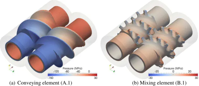
The pressure distribution on the surface of the twin-screw extruder for cases (A.1) and (B.1) is shown in Figure 7. Note that the exit pressure is taken as a reference and it was fixed to 0 in the numerical simulation. The magnitude of the pressure changes along the screw is much more important for the conveying element as the openings present in the mixing element allows the material to flow more easily. The pressure evolution on the surface of the barrel along the line y = 0, z = -Δz/2-R for various operating conditions is shown in Figure 8. Figure 8(a) indicates an
18 increase in the magnitude of the pressure change along the screw when the rotation speed increases as the larger velocities more than offset the decrease in the viscosity. The influence of the feed rate and of the screw element type is shown in Figure 8(b). Pressure changes are much smaller for the mixing element than for the conveying element. Note also that the pressure increase along the screw element is larger for the smaller feed rate. This is determined by the fact that a higher flow rate is associated with a higher upstream pressure. On top of that we have the pressure changes determined by the screw rotation which generates an increase of the pressure in the flow direction.
(a) Conveying element (A.1) (b) Mixing element (B.1)
Figure 7: Pressure distribution on the screws surface for the cases A.1 and B.1
(a) Effect of rotation speed (A.1, A.3, A.4) (b) Effect of element type and feed rate
19
4.2. Mixing behavior of screw elements
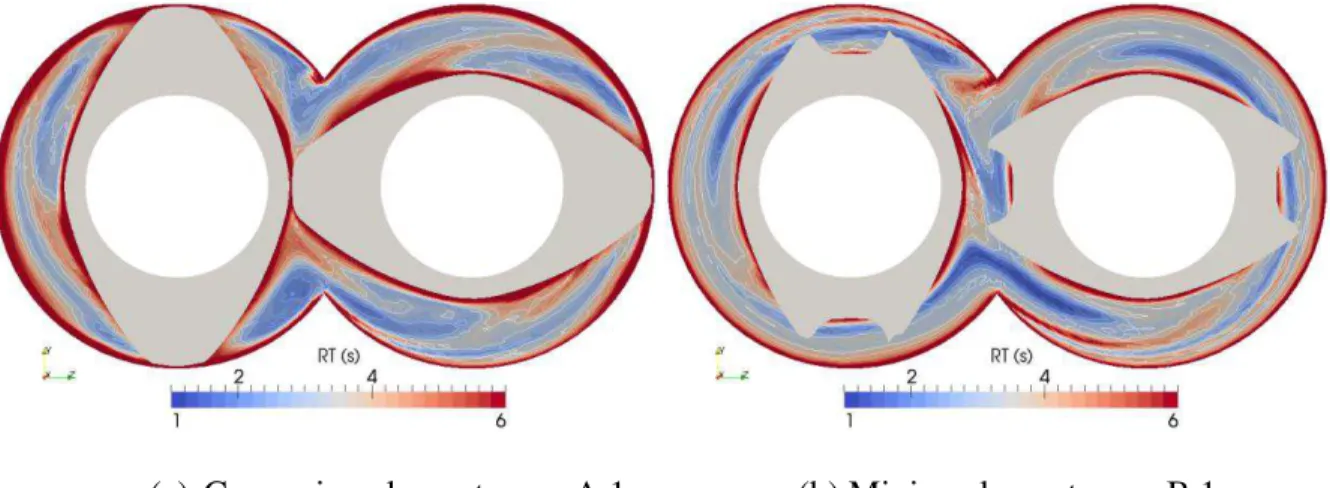
In this section the mixing behavior of the conveying and mixing screw elements is compared. Figure 9 shows the residence time distribution E(t) for the screw rotating at 120rpm as determined by the tracking of 17,600 particles entering the screw element region at different times and at various locations. One can observe that the mixing element presents a lower maximum value of the residence time distribution and also a larger range of residence time values containing a significant number of particles. This effect is more evident for the larger feed rate case shown in Figure 9(b). The spatial distribution of the residence time at the exit of the screw elements as given by the transport equation (12) is shown in Figure 10. As expected the larger residence time is observed in the layers close to the screw and barrel surface as the polymer melt sticks to the solid surface and therefore remains a longer period of time inside the screw region. At the opposite, a shorter residence time is obtained for the polymer at the core of the region between the screw and the barrel.
(a) Feed rate of 3.375 kg/h (b) Feed rate of 6.75 kg/h
20 (a) Conveying element, case A.1 (b) Mixing element, case B.1
Figure 10: Spatial distribution of the residence time for conveying and mixing elements
The length stretch analysis was performed for different values of the initial distance between the tracked points (initial size of a single cluster) in order to determine the influence of this parameter on the numerical results. Results are shown in Figure 11 for an initial distance between points in a cluster δ ranging from 0.0025mm to 0.04mm. For times up to 0.6s in the case A.1 and up to 0.8s in the case ψ.1 all results are very close to each other indicating no dependence on δ. Recall, that for cases A.1 and B.1 the screws rotate at 120rpm, so the rotation period is 0.5s. For longer times the solution for the larger value of δ is slightly different, but little difference is observed for the smaller values of δ. Therefore, we selected δ=0.005mm for the length stretch analysis. The average length stretch evolution with time for conveying and mixing elements is shown in Figure 12 for the two feed rates considered. In both cases, after an initial period of time of about 0.4s during which the average length stretch is similar for the two element types, the average length stretch becomes larger for the mixing element than for the conveying element, thus indicating a better mixing capacity for this type of screw element.
21 (a) Conveying element, A.1 (b) Mixing element, B.1
Figure 11: Average length dependence on the initial distance between points
(a) Feed rate of 3.375 kg/h (b) Feed rate of 6.75 kg/h
Figure 12: Average length stretch evolution with time
The length stretch distribution as given by Eq. (14) is shown in Figure 13 after two complete screw rotations (t=1s). The curve corresponding to the conveying element is shown with a continuous line, whereas the one for the mixing element is plotted with a discontinuous line. As can be seen, for both feed rates the conveying element has a larger number of particle pairs exhibiting a low length stretch, with more pairs experiencing high length stretch for the mixing element. The crossing point for the two curves is at about λc=30 for the lower feed rate and about
22 λc=20 for the higher feed rate. It means that, at t=1s, the number of pairs experiencing a length stretch higher than λc is larger for the mixing element than for the conveying element.
(a) Feed rate of 3.375 kg/h (b) Feed rate of 6.75 kg/h
Figure 13: Length stretch distribution at t=1s
Another way to study the mixing behavior of screw elements is two follow a large number of particles initially located very close to each other along a line segment. This gives us the possibility to illustrate how the respective line segment is deformed by the flow. As for the particle tracking used to determine residence time and length stretch, here we consider that particles travel with the same velocity as that of the polymer melt, do not interact to each other and are not affecting the flow. Here we present results when tracking 10,000 particles initially forming a line segment of 5mm length found at x=7.5mm, z=0, between y=0 and y=5mm. The line formed by the tracked particles is shown at different times in Figure 14 for cases A.1 and B.1. The distance between two successive particles is initially of 0.0005mm, but increases with time and may reach quite large values indicating a dispersion of the material from one specific location to various regions of the screw volume. Once the distance between two successive particles reaches 2mm we consider that the imaginary link between these particles is broken and the line becomes discontinuous at this location. Figure 14 clearly indicates that the mixing element produces a far more important dispersion of particles inside the flow domain.
23 (a.1) Conveying element, t = 0 (a.2) Mixing element, t = 0
(b.1) Conveying element, t = T/2 (b.2) Mixing element, t = T/2
(c.1) Conveying element, t = T (c.2) Mixing element, t = T
(d.1) Conveying element, t = 3T/2 (d.2) Mixing element, t = 3T/2
(e.1) Conveying element, t = 2T (e.2) Mixing element, t = 2T
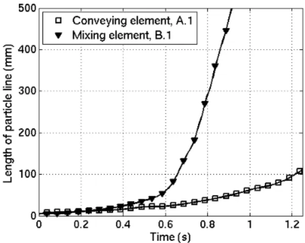
24 The total length of the line segments formed by the tracked points (without including those segments longer than 2mm) is shown in Figure 15. The results indicate a far better mixing in the case of the mixing element screw when compared with the conveying element screw. After an initial period up to 0.6s during which the total length is only slightly larger for the mixing element and for which we have no line break, the two types of screw behave very differently with the mixing element showing a sharp increase in the total length. This is again evidence of the better mixing behavior of this type of screw.
Figure 15: Evolution of the line of particles with time
5. CONCLUSION
This work presents the application of a numerical approach to study the mixing behavior of various screw elements based the flow solution given by an IB method. The IB finite element method accurately imposes the boundary conditions on the fluid/solid interface and provides solutions for the isothermal flow inside co-rotating twin-screw extruders. The procedure consists of incorporating into the grid the points where the mesh intersects the boundary. The degrees of freedom associated with the additional grid points are then eliminated either because the velocity is known or by static condensation in the case of the pressure.
25 The polymer melt is considered to behave as a generalized Newtonian fluid and flow solutions indicate that velocity profiles are affected by the shear thinning behavior of the material. The pressure drop along the screw depends on the screw rotation speed, feed rate and screw type. The pressure buildup between the exit and entry of a screw element increases when increasing the screw rotation speed and is much more important for a conveying element than for a mixing element.
The time-dependent 3D flow solution was then used to compute mixing parameters such as the residence time and length stretch distribution. Numerical results indicate that the residence time is more uniform for the conveying element and that the length stretch is larger for the mixing screw element. The tracking of a large number of particles initially located along a line segment indicated a much better mixing capacity for the mixing element. Both the total line length and the number of line parts increases faster in the case of the mixing element.
REFERENCES
Bertrand, F., et al., “Adaptive finite element simulations of fluid flow in twin-screw extruders”, Comp. Chem. Eng., 27, 491-500 (2003), DOI:10.1016/S0098-1354(02)00236-3
Bravo, V.L., et al., “Numerical simulation of pressure and velocity profiles in kneading elements of a co-rotating twin screw extruder”, Polym. Eng. Sc., 40, 525-541 (2000), DOI:10.1002/pen.11184
Cheng, H., Manas-Zloczower, I., “Study of mixing efficiency in kneading discs of co-rotating twin-screw extruders”, Polym. Eng. Sc., 37, 1082-1090 (1997), DOI:10.1002/pen.11753
Cheng, H., Manas-Zloczower, I., “Distributive mixing in conveying elements of a ZSK-53 co-rotating twin screw extruders”, Polym. Eng. Sc., 38, 926-935 (1998), DOI:10.1002/pen.10260
26 Franca, L.P., Frey, S.L., “Stabilized finite element methods: II. The incompressible Navier-Stokes equations”, Comp. Methods Appl. Mech. Eng., 99, 209-233 (1992), DOI:10.1016/0045-7825(92)90041-H
Hughes, T.J.R., et al., “A new finite element formulation for computational fluid dynamics: V. Circumventing the Babuška-Brezzi condition: A stable Petrov-Galerkin formulation of the Stokes problem accommodating equal-order interpolations”, Comput. Methods Appl. Mech. Engrg., 59, 85-99 (1986), DOI:10.1016/0045-7825(86)90025-3
Ilinca, F., Hétu, J.-F., “A finite element immersed boundary method for fluid flow around rigid objects”, Int. J. Numer. Methods Fluids, 65, 856-875 (2011), DOI.10.1002/fld.2222
Ilinca, F., Hétu, J.-F., “A finite element immersed boundary method for fluid flow around moving objects”, Comput. Fluids, 39, 1656-1671 (2010a), DOI:10.1016/j.compfluid.2010.06.002 Ilinca, F., Hétu, J.-F., “Three-dimensional finite element solution of the flow in single and twin-screw extruders”, Int. Polym. Proc., 25, 275-286 (2010b), DOI:10.3139/217.2351
Ilinca, F., Hétu, J.-F., “Three-dimensional filling and post-filling simulation of polymer injection moulding”, Int. Polym. Process., 16, 291-301 (2001)
Ilinca, F., Hétu, J.-F., “Three-dimensional numerical modeling of co-injection molding”, Int. Polym. Process., 17, 265-270 (2002)
Ilinca, F., Hétu, J.-F., “Three-dimensional finite element solution of gas-assisted injection moulding”, Int. J. Numer. Methods Eng., 53, 2002-2017 (2003)
Ishikawa, T., et al., “3-D Numerical simulations of nonisothermal flow in co-rotating twin screw extruders”, Polym. Eng. Sc., 40, 357-364 (2000), DOI:10.1002/pen.11169
Kajiwara, T., et al., “Numerical study of twin-screw extruders by three-dimensional flow analysis - Development of analysis technique and evaluation of mixing performance for full flight screws”, Polym. Eng. Sc., 36(16), 2142-2152 (1996), DOI:10.1002/pen.10611
27 Kalyon, D.M., Malik, M., “An integrated approach for numerical analysis of coupled flow and heat transfer in co-rotating twin screw extruders”, Int. Polym. Process., 22, 293-302 (2007) Lawal, A., Kalyon, D.M., “Mechanisms of mixing in single and co-rotating twin screw extruders”, Polym. Eng. Sci., 35, 1325-1338 (1995)
Malik, M., Kalyon, D.M., “3D Finite element simulation of processing of generalized Newtonian fluids in counter-rotating and tangential TSE and die combination”, Int. Polym. Process., 20, 398-409 (2005)
Ottino, J.M., et al., “A framework for description of mechanical mixing of fluids”, AIωhE J., 27, 565-577 (1981), DOI:10.1002/aic.690270406
Speur, J.A., et al., “Flow patterns in calender gap of a counterrotating twin screw extruder”, Adv. Polym. Tech., 7, 39-48 (1987), DOI:10.1002/adv.1987.060070105
Yao, C.-H., Manas-Zloczower, I., “Influence of design on dispersive mixing performance in an axial discharge continuous mixer – LωMAX 40”, Polym. Eng. Sc., 38(6), 936-946 (1998), DOI:10.1002/pen.10261
Zhang, X.-M.,et al., “Numerical simulation and experimental validation of mixing performance of kneading discs in a twin screw extruder”, Polym. Eng. Sc., 49(9), 1772-1783 (2009), DOI:10.1002/pen.21404