Asymptotically good convolutional codes with feedback encoders

Asymptotically Good Convolutional Codes with

Feedback Encoders

by

Peter J. Sallaway

Submitted to the Department of Electrical Engineering and

Computer Science

in partial fulfillment of the requirements for the degree of

Bachelor of Science in Electrical Engineering and Computer Science

and Masters of Engineering in Electrical Engineering and Computer

Science

at the

MASSACHUSETTS INSTITUTE OF TECHNOLOGY

June 1997

@ Peter J. Sallaway, MCMXCVII. All rights reserved.

The author hereby grants to MIT permission to reproduce and

distribute publicly paper and electronic copies of this thesis and to

grant others the right to do so.

OCT 291997

LIRSACFtES

Author ...

...

Department of Electrical Engineering and Computer Science

May 23, 1997

Certified by ... ...

..

...

Amos Lapidoth

Assistant Professor

Accepted by ...

-rroiessor Ar

unur

%.

.

1111mL

Chairman, Departmental Committee on Graduate Students

Asymptotically Good Convolutional Codes with Feedback

Encoders

by

Peter J. Sallaway

Submitted to the Department of Electrical Engineering and Computer Science on May 23, 1997, in partial fulfillment of the

requirements for the degree of

Bachelor of Science in Electrical Engineering and Computer Science and Masters of Engineering in Electrical Engineering and Computer Science

Abstract

The results of a computer search for convolutional encoders for the binary symmetric channel and the additive white Gaussian noise channel are reported. Both feed-forward and feedback encoders are considered, and it is shown that when the bit error rate is the design criteria feedback encoders may outperform the best feed-forward encoders at no additional complexity.

Thesis Supervisor: Amos Lapidoth Title: Assistant Professor

Acknowledgments

I would like to thank G.D. Forney, M.D. Trott and G.C. Verghese for helpful discus-sions and Amos Lapidoth for his assistance throughout.

Contents

1 Introduction

1.1 Digital Communication Systems . . . . 1.2 Error Correcting Codes ...

1.3 Communications Channels . . . .

2 Convolutional Encoders

2.1 Definitions . ...

2.2 The Structure of a General Encoder . 2.3 Alternative Representations ... 2.4 Distance Properties ... 2.5 Classes of Encoders ... 2.6 The Viterbi Decoder ... 2.7 Performance Analysis ... 3 Results 4 Conclusion A Corrections to [16] B Corrections to [7] C Tables D Extended Tables 12 . . . . 13 . . . . 13 . . . . 17 . . . . 19 . . . . 2 1 . . . . 23 . . . . 24 26 30 32 33 38

List of Figures

1-1 A digital communications system. ... .. 8

2-1 A controller form realization of a rate k/n convolutional encoder. . . 14 2-2 Representation of an encoder as a precoder followed by a feed-forward

encoder. ... 16

2-3 Implementation of a rate 2/3 convolutional encoder. . ... 16 2-4 A rate 1/2 feed-forward convolutional encoder. . ... 17 2-5 The state diagram of a rate 1/2 feed-forward convolutional encoder.. 18 2-6 The trellis diagram of a rate 1/2 feed-forward convolutional encoder. 18 2-7 The modified state diagram of a rate 1/2 feed-forward convolutional

encoder ... ... 21

4-1 Simulation results of rate 2/3 encoders with 64 states (m = 6) on the AW GN channel ... .... 29

List of Tables

C.1 Asymptotically good rate 1/2 encoders on the BSC

C.2 Asymptotically good rate 1/2 encoders on the AWGN C.3 Asymptotically good rate 1/3 encoders on the BSC . C.4 Asymptotically good rate 1/3 encoders on the AWGN C.5 Asymptotically good rate 2/3 encoders on the BSC . C.6 Asymptotically good rate 2/3 encoders on the AWGN D.1 D.2 D.3 D.4 D.5 D.6 D.7 D.8 channel channel channel Rate 1/2 encoders on the BSC ...

Rate 1/2 encoders on the AWGN channel. Rate 1/3 encoders on the BSC ... Rate 1/3 encoders on the AWGN channel. Rate 2/3 encoders on the BSC ... Rate 2/3 encoders on the BSC ... Rate 2/3 encoders on the AWGN channel. Rate 2/3 encoders on the AWGN channel.

. . . . 39 S . . . . . 40 . . . . 41 . . . . . 42 . . . . 43 . . . . 44 . . . . . 45

. . . .

.

46

Chapter 1

Introduction

In today's society, reliable communication systems transmit an enormous quantity of digital data. These systems often must transmit and reproduce data with bit error rates of 10-12 and below[2]. A communication system is required to achieve this performance despite the presence of various types of noise. In order to overcome noise, a variety of techniques are used.

Repeating messages and increasing the strength of the signal are two classical methods of overcoming an unreliable communications channel. Repetition results in communications with a reduced transmission rate, increased bandwidth, or a com-bination of both. Alternatively, increasing signal strength requires an increase of power consumption, which is often limited by battery power or interference. These techniques are often impractical as transmission rate, bandwidth, and power are too important to be sacrificed. In modern communication systems, another approach is taken to solve this problem. Error correcting codes use complicated message struc-tures, with detailed cross checks, to improve reliability while minimizing the sacrifices of rate, bandwidth and power[2]. These techniques require sophisticated transmitters and receivers to encode and decode messages. However, the increased implementation complexity is more than offset by the gains in performance.

Noise

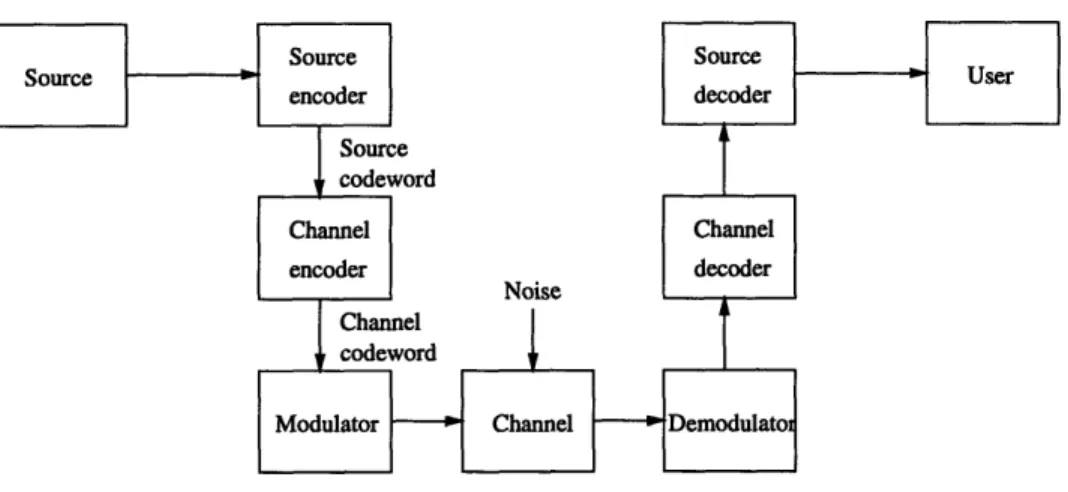
Figure 1-1: A digital communications system.

1.1

Digital Communication Systems

The study of error correcting codes began in 1948 following a paper by Claude Shannon[21]. Shannon showed that a communications channel limits the rate and not the accuracy of data transmission. As a result, we have learned that data trans-mission up to a particular rate, defined as the capacity of a channel by Shannon, can achieve an arbitrarily low probability of output error. Although Shannon proved that this is possible, he did not enlighten us on how to find such coding techniques.

Almost 50 years after Shannon's original work, digital communication systems are still trying to approach Shannon's limit. Figure 1-1 depicts a typical digital communi-cations system. The data is initially encoded by a source encoder. The source encoder removes redundancy within the data, representing it more compactly. The resulting source codeword is then encoded by a channel encoder. The channel codeword is a longer sequence than the source codeword, containing designed redundancy. The modulator then converts each channel symbol into its corresponding analog symbol. This sequence of analog symbols is transmitted over the channel. As a result of noise within the channel, the channel output differs from the channel input. The demodu-lator translates the received analog signal into quantized data. This data is received

by the channel decoder, which then produces an estimate of the source codeword. The source decoder then inverts the operation done by the source encoder to produce the output data.

1.2

Error Correcting Codes

Within a digital communications system, the design of the channel encoder and de-coder is known as the study of error correcting codes. There are two basic types of error correcting codes, block codes and convolutional codes. Block codes encode fixed length blocks of information independently. Conversely, convolutional encoders encode a sequence of symbols as a whole. Convolutional encoding depends on both current information symbols as well as a set of past information symbols. As we will be dealing exclusively with channel encoders and channel decoders from now on, they will be referred to as simply the encoder and the decoder.

Both convolutional encoders and block encoders add redundancy to the informa-tion sequences, thus the set of possible codewords, the code, contains only a subset of all possible sequences. The distinction between a code and an encoder must be emphasized. The code is defined as the set of possible output sequences from the encoder. The encoder is defined as the set of input/output relationships between the entire spectrum of inputs and the code. Furthermore, Massey and Sain [17] defined two encoders equivalent if they generate the same code. Equivalent encoders are distinguishable by their mappings from the input sequences to the code.

Decoders use the redundancy in the codewords to correct errors caused by the channel. Two groups of decoders, hard decision decoders and soft decision decoders, are differentiated by the set of data that they receive from the demodulator. A hard decision decoder receives an estimate of the channel codeword in order to decode the source codeword. A soft decision decoder receives more information than just this estimated channel codeword. The additional data can be considered an indication of the reliability of each symbol within the estimated codeword. Thus in general, a soft decision decoder performs better than a hard decision decoder.

1.3

Communications Channels

The errors facing a decoder can be modeled as errors from two sources, channels with memory and channels without memory. Memoryless channels, where each transmitted symbol is affected by noise independently of the others, produce random errors. On the other hand, channels with memory will often produce burst errors. They tend to produce long periods with virtually errorless transmission and occasional periods where the channel error probability is very high. These bursts often result in erasures or useless data.

Error correcting codes are much better at handling random errors than burst er-rors. Therefore, a commonly used technique to deal with burst errors is interleaving[7], which has the effect of spreading the burst errors such that they appear to be ran-dom errors. Block codes and convolutional codes focus on correcting ranran-dom errors resulting from memoryless channels.

The memoryless channels that we will be using are the Binary Symmetric Channel (BSC) and the Additive White Gaussian Noise (AWGN) channel. The BSC models a binary channel with hard decision decoding where each symbol, a 'O0' or a '1', is received by the decoder correctly with probability (1 - p), and incorrectly with

probability p. The AWGN channel is used to model a channel with a soft decision decoder. The noise is assumed to be a zero mean white Gaussian random process. The output of the AWGN channel is the sum of the analog input signal and the white Gaussian noise. Thus on the AWGN channel the demodulator gives more detailed data to the decoder than it does over the BSC.

In this study, we are going to report the results of a computer search for convo-lutional encoders with low bit error rates (BER) over the BSC and AWGN channel. This search will consist of a more broad range of convolutional encoder than the traditionally studied feed-forward encoders by including encoders which take advan-tage of feedback. It will be demonstrated that when BER is the design criteria, non feed-forward encoders may outperform feed-forward encoders with comparable code parameters. In order to do this, we must first look more closely at convolutional

Chapter 2

Convolutional Encoders

[8] showed that every convolutional encoder is equivalent to a feed-forward encoder, i.e., an encoder with a finite impulse response. In other words, every encoder produces the same code as a feed-forward encoder. It can be seen that if all input sequences are equally likely (as we shall assume throughout) then the probability of a sequence error, i.e., the probability that the reconstructed sequences differs from the input sequences, depends only on the set of possible output sequences (the code) and not on the input/output relationship. Forney

In view of the above results, much of the literature on convolutional encoders has focused on feed-forward encoders, and most searches for good convolutional encoders were limited to feed-forward encoders [19, 15, 20, 12, 5, 4, 16, 11]. See however [14] where a different class of encoders was considered, the class of systematic encoders1_.

While the message error rate does indeed depend only on the code, the BER depends not only on the code but also on the encoder. Two equivalent encoders may thus give rise to a different BER over identical channels. For applications where BER is of concern rather than message error rate, e.g. in some voice modem applications, non feed-forward encoders may thus be preferable.

2.1

Definitions

A binary rate k/n convolutional encoder is a k-input n-output causal linear time-invariant mapping over GF(2) that is realizable using a finite number of states [8]. Using the D-transform we can describe the input to a convolutional encoder as a k row vector, x(D), whose entries are the D-transforms of the input sequences

zi(D)

=

xi,tDt 1 < i < k.

t

Similarly, we can describe the output as a n row vector, y(D), whose entries are the D-transforms of the output sequences

yj(D)=

yj,tD

t

_{1 < j < n.}

t

With this notation, we can describe a convolutional encoder using a k x n transfer function matrix G(D) whose entries are rational functions in D such that

y(D) = x(D)G(D).

For a feed-forward convolutional encoder, the transfer function matrix contains entries which are restricted to polynomials in D.

2.2

The Structure of a General Encoder

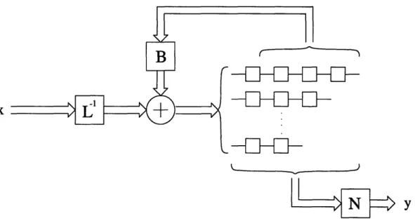
A realization of an encoder is said to be minimal if the encoder cannot be realized with fewer states. It can be shown that for any encoder one can find a minimal realization in controller form, as depicted in Figure 2-1[13].

The generator matrix G(D) is thus represented as

G(D) = L-1 (B(D) + I)-'N(D),

-in

]-EIJ-

1-X

NJ

Y

Figure 2-1: A controller form realization of a rate k/n convolutional encoder. entries, each divisible by D; and N(D) is a k x n polynomial matrix. The number of states in this realization is 2m where m is the number of state variables (delay elements) and

k

m = mi,

i=1

and

mi = max max degBi(D), max degNij(D)}. (2.1)

(1<h<k 1<j<_n

The encoder itself is defined to be minimal if the minimum number of states required to realize the encoder is no larger than the number of states required to realize any other encoder that generates the same code2_{. If the encoder is minimal,}

then it can be shown that

max degBih(D) < max degNij(D),

1<h<k 1<j<n

2

This notion of encoder minimality should not be confused with the notion of a minimal realization of an encoder, which was defined earlier in this section.

so that (2.1) can be replaced by

mi = max degNij(D).

As an example, consider the rate 1/n case. Here L is an invertible binary scalar and is thus one. The matrix B(D) is also 1 x 1 and is thus simply a polynomial divisible by D. Finally N(D) is an n row vector of polynomials. The generator matrix is thus

G(D) = B(D)+1 [ Ni (D) N2(D) ... N,(D) .

To within a constant delay the encoder G(D) can be thought of as the cascade of a (B(D) + 1)-1 precoder followed by a feed-forward convolutional encoder with generator matrix N(D). On the receiver end, decoding can be performed using a Viterbi decoder3 tuned to the feed-forward part and then running the result through the finite impulse response (FIR) filter B(D) + 1. This implementation may have merit if an off-the-shelf Viterbi decoder is to be used.

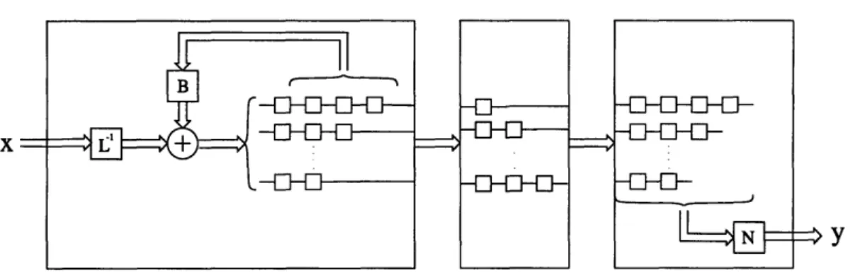
The general rate k/n encoder is slightly more complicated, but with analogous results. Once again, to within a constant delay, we can view the encoder as a cascade of a k x k precoder L-1(B(D) + I)-1, a feed-forward encoder with a polynomial generator matrix N(D), and a diagonal delay matrix in between, see Figure 2-2. Decoding can be performed by Viterbi decoding the feed-forward encoder and then running the resulting sequences through the FIR system (B(D) + I)L.

An example of a rate 2/3 convolutional encoder with m = 4 state variables (16 states) is depicted in Figure 2-3. The generator matrix for this encoder is

1 D2 1+D

G(D)=

1+D+D

2

1+D+D

2 0 1+D 1+D+D 2 D 2 1+D j

-El---E-El--ý

Figure 2-2: Representation of an encoder as a precoder followed by a feed-forward encoder.

yl(D)

y2(D)

y3(D)

Figure 2-3: Implementation of a rate 2/3 convolutional encoder. Here, G(D) is implemented with

,B(D) = D + D2

0

,N(D) =

1+D+D

2

0 1+D2 1+

In order to simplify notation, we shall follow [16] and use octal notation with D = 2. Thus we can write

,N(D) =

0

141

5 7

x,(D) x2(D) 02 D+D 2

B

+ IHII

x 6 B(D) =

0

xl(D)

y,(D)

y2(D)

Figure 2-4: A rate 1/2 feed-forward convolutional encoder.

2.3

Alternative Representations

A better understanding of the convolutional encoding operation can be achieved by developing further graphical representations of the encoder. The state diagram and the trellis diagram help us analyze the performance and decoding of convolutional encoders. A convolutional encoder can be represented as a finite state machine. To see this representation let us look at an example of a simple rate 1/2 feed-forward convolutional encoder. The controller form realization is depicted if Figure 2-4, where we can see that G(D) = [1+D2 1+D + D2 . The contents of the memory

elements are called the state of the encoder. This rate 1/2 encoder requires two memory elements, m = 2, and hence has four states. Each state has 2k branches

entering and leaving it, in this example there are two. The state diagram is shown in Figure 2-5. Each state is circled, with the most recent input bit as the least significant bit in the state. The branches denote the possible transition from one state to another. Each branch is labeled with the input/output bits. With this representation of the encoder, we can more readily find its distance properties which give us insight to the encoder's performance.

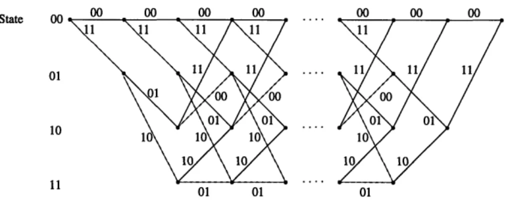
The trellis diagram is a very common representation of a convolutional encoder. The trellis diagram for the encoder in Figure 2-4 is depicted in Figure 2-6. Again, there are four states with two branches entering and leaving each. Let us assume we start and end in the all zero state. Each branch is again labeled with the corresponding output bits of that transition. A dashed branch corresponds to an input bit '1' and a solid branch corresponds to a 'O'. This representation will be very helpful when analyzing the Viterbi decoder.

1/10

1/11 0/11

Figure 2-5: The state diagram of a rate 1/2 feed-forward convolutional encoder.

State 00

01

10

01 01 01

Figure 2-6: The trellis diagram of a rate 1/2 feed-forward convolutional encoder.

2.4

Distance Properties

The error correcting capabilities of the code, as well as the resultant BER using various types of decoders, can be determined or bounded using the free distance and distance spectrum of an encoder. The free distance, df, is the minimum Hamming distance between any two codewords. As a result of the linearity of convolutional codes, this is also the weight of the minimum weight nonzero codeword. The error correcting capability of a code is therefore [df2j. We can use the state representation of an encoder to help calculate the free distance. By considering the weight of each transition as the Hamming weight of the output bits of the corresponding branch, we find the free distance as the minimum weight of any path which starts and ends at the all zero state and visits at least one other state. Using the state diagram in Figure 2-5, we can find the free distance of the encoder in Figure 2-4 is df = 5. Please note that the free distance is a function solely of the code and not the particular encoder which realizes it.

Another important distance property of a code is its distance spectrum. The number of codewords of each specific weight helps determine the performance of an encoder using Viterbi decoding. Let us define n(df + i) as the number of codewords of weight df + i. We can then define the distance spectrum as the sequence

n(df + i), i =

0,

1, 2, ...

Again, the distance spectrum is solely a function of the code, not the encoder. A related sequence is the total number of nonzero information bits, nb(df + i), in all

weight df + i codewords. Because this sequence requires knowledge of both the input and the output of a particular transition from one state to another, it is not only a function of the code, but also of the encoder. This sequence is used to calculate an upper bound to the BER with Viterbi decoding on both the BSC and AWGN channel.

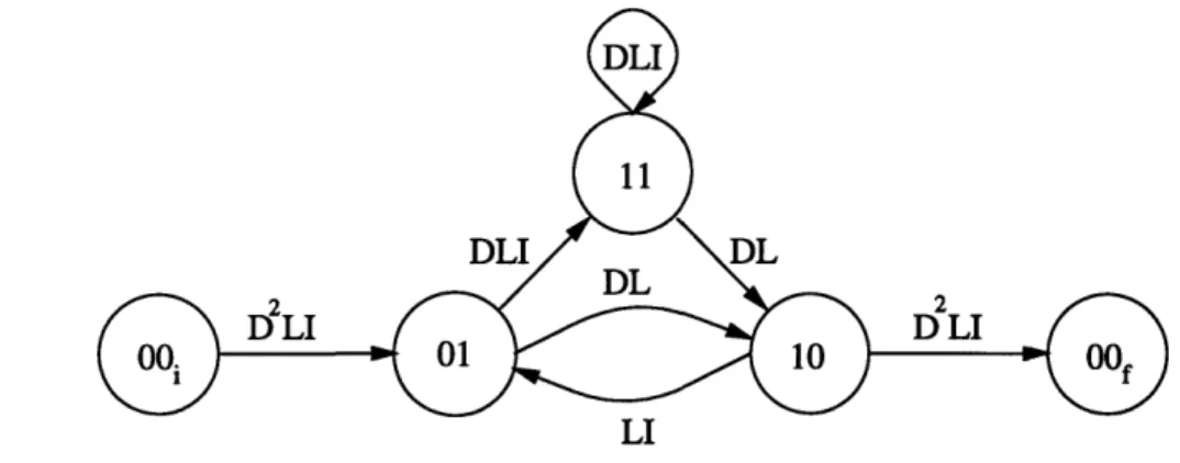
Trans-fer Function4. The Transfer Function can be found using a modified encoder state diagram. Let the all zero state be broken up into an initial and final state. By again using the encoder in Figure 2-4, we can see the resulting state diagram in Figure 2-7. The branches of the state diagram are labeled with three parameters. The exponent of D indicates the weight of the encoded branch. The exponent of I indicates the weight of the information branch. The exponent of L indicates the length of the path. The Transfer Function is given by

T(D, L, I) = E Ad,l,iDdLLIi,

d,1,i

where Ad,l,i is the number of codewords of weight d, whose associated information sequence has weight i, and whose length is 1.

T(D, L, I) can be computed by considering a walk through this modified state

diagram, beginning an the initial all zero state and ending at the final all zero state. The simultaneously state equations gained from the walk through Figure 2-7 are

0ol = D2LIp0oo + LIOo1

il1o = DLVol + DL' 11

011 = DLIol + DLI011

0oof = D2_L0 10

where O's are dummy variables for partial paths to the intermediate states. The initial and final all zero states are ioo0 and ?0oof respectively. The Transfer Function can be defined as

T(D, L, I) - 'oof

000i

By solving these simultaneous equations about, we find

T(D, L, I) D5L'I

S1-DLI(L+1)

= D5L31 + D6L412 (L + 1) + ... + Dk+5Lk+3Ik+l(L + 1)k +

4

This Transfer Function should not be confused with the transfer function matrix, G(D), which was discussed in Section 2.1

DLI

Figure 2-7: The modified state diagram of a rate 1/2 feed-forward convolutional encoder.

A simplified Transfer Function obtained by setting L = 1 and I = 1 is given by

T(D) = AdDd.

d

The expansion of this simplified Transfer Function gives us the distance spectrum, with Ad codewords of weight d. By using our Simplified Transfer function with L = 1 and I = 1, we find

D5

T(D) 1 D= D + 2D 6 + 4D7 + ... + 2kDk+5 ..

1 - 20D

Therefore, there is one codeword of weight five, two codewords of weight six, four codewords of weight seven, etc, thus determining our distance spectrum. We can also only set L = _{1 and use T(D, I) to determine nb(df + i).}

Before using our distance statistics to analyze the performance of an encoder, let us look at two important classes of convolutional encoders, catastrophic and systematic encoders, and examine the decoding process of interest, Viterbi decoding.

2.5

Classes of Encoders

One class of convolutional encoders to be avoided, are catastrophic encoders. A catastrophic encoder has the property that it is possible for a finite number of channel

errors to produce an infinite number of decoding errors, an obviously undesirable result. We can determine whether or not an encoder is catastrophic by looking at its transfer function matrix G(D). Let us first look at the catastrophicity of a feed-forward encoder and then extend our results to the general encoder.

As mentioned earlier, for a feed-forward encoder, each entry in the transfer func-tion matrix G(D) is polynomial in D. In this case, [17] states that we can declare a code non-catastrophic if and only if

gcd [A(D),i= 1, 2,..., D',

for some nonnegative integer 1, where Aj(D), 1 <i < (n), are the determinants of

the (k) distinct k x k minors of G(D). We can see that for the rate 1/n feed-forward

encoder, if there is a non-trivial common divisor to the entries of G(D) then the code is catastrophic.

We will show that in the general case, where G(D) contains rational entries, we can use the controller form realization described earlier, with G(D) = L-1(B(D) + I)-'N(D), to state that G(D) is catastrophic if and only if the feed-forward encoder N(D) is catastrophic. We have demonstrated that the encoder G(D) can be

repre-sented as a precoder of the form L- 1(B(D)+I)- 1 _{followed by the feed-forward encoder}

N(D), and that decoding can be performed by Viterbi decoding on the feed-forward

encoder, with the resulting sequences running through the FIR system (B(D) + I)L. Because the postcoding filter has a FIR, it will have no affect on the catastrophicity. Therefore it follows that G(D) is catastrophic if and only if the feed-forward encoder

N(D) is catastrophic, a condition that can be checked using the standard techniques

of [17].

One subset of convolutional encoders that are not catastrophic are systematic encoders. Systematic encoders transmitted the data symbols unchanged within the coded symbols. The transfer function matrix can be shown as G(D) = [I: G'(D)]

where I is the k x k identity matrix and G'(D) is a k x (n - k) matrix with rational entries in D. An advantage of a systematic encoder is that if there are no errors,

the information sequence can be easily recovered. It can be shown [6] that every convolutional encoder is equivalent to a systematic encoder. However, systematic encoders where G'(D) contains only polynomials in D, i.e. feed-forward systematic encoders, have distance properties that have been shown to be inferior to those of non-systematic encoders with equal rate and memory length. Inferior distance properties result in encoders with poor performance when using Viterbi decoding.

2.6

The Viterbi Decoder

The most commonly used decoding algorithm is the Viterbi algorithm. The Viterbi decoder is a maximum likelihood sequence decoder for convolutional codes[22]. This decoder chooses the codeword which has the highest probability of being transmitted based upon the received sequence. The advantage of the Viterbi algorithm is its efficiency, which is obtained by using dynamic programming techniques. The Viterbi algorithm recognizes that it is unnecessary to consider the entire received sequence when deciding upon early segments of the most likely transmitted sequence. By referring to the trellis diagram representation, we may conclude that we can eliminate segments on non-maximum probability paths when paths merge. No matter the future received symbols, they will affect the probability only over subsequent branches after these paths have merged, and consequently in exactly the same manner. Therefore, as paths merge, it is only necessary to remember the maximum probability path at each of the 2k states, called the survivor. In this manner, we can proceed through the trellis preserving only one surviving path at each state, for each unit of time. Over the BSC, the path of maximum probability will have the minimum Hamming distance between itself and the received sequence. The resulting decoding complexity has been reduced to grow linearly with the sequence length and the number of states. Without the dynamic programming used within the Viterbi algorithm, the complexity would grow exponentially with the sequence length. The Viterbi algorithm is efficient enough to be practical in most applications. Thus it is important to understund the performance of a convolutional encoder with Viterbi decoding.

2.7

Performance Analysis

The exact BER incurred when a convolutional encoder and a Viterbi decoder are used over a noisy channel is generally very difficult to obtain, however see [3, 1] for an asymptotic performance analysis on the BSC. On the Gaussian channel things are a little more complicated as we do not know the precise asymptotics of the BER.

In order to examine the BER, we must first look at the pairwise error probability,

Pd. The pairwise error probability is defined as the probability of decoding incorrectly

when one of two codewords is transmitted with Hamming distance d. On the BSC, we can see that

j

= ()

Pb

_ bdb d odd

2

P

1

d

pd/2

d/2

d

₍

pb

_d-b

and on the AWGN channel

Pd= Q U

where cr2 _{is proportional to the variance of the additive noise. By taking the sum of}

the pairwise error probability of all codewords, with respect to the all zero codeword, it can be shown [22] that the BER, Pb, for a rate k/n encoder can be upper bounded by

Pb < -E

E

ia(d, i)Pd,

i=l d=df

where a(d, i) is the number of paths diverging from the all zero path at a particular time with distance d and corresponding information weight i. Please note that a(d, i) are the coefficients of the Transfer Function T(D, L, I) with L = 1. This bound is commonly referred as the Transfer Function bound.

probability p the BER [16] is given by5 1

Pb = -ABscPd + O(pd+l) (2.2)

with

d= df+1 , (2.3)

and where df is the code's free distance. Here the coefficient ABSC can be computed precisely as described in [16]. However, on the AWGN channel we can no better than the Transfer Function bound. It is thus shown for high signal to noise ratios [22],

[10], [9], [18] that the BER is bounded by

Q(

<BER

< Q W

,

(2.4)

where 0 is the combined Hamming weight of all the data sequences that correspond to error events that are of encoder output weight df. Thus 3 is the coefficient of the first term in the Transfer Function bound on the encoder's BER [22].

In this study, we have searched for the encoder that minimizes (2.2) at very low crossover probabilities p and for the encoder that minimizes the upper bound in (2.4) at very low noise variances.

5_{The term 1 was apparently overlooked by Lobanov. We do not incorporate it into the constant}

ABSC so that our tables for rate 2/3 will agree with Lobanov's. Please refer to Appendix A for a more detailed discussion.

Chapter 3

Results

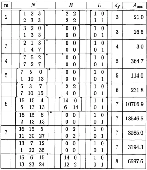
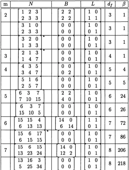
We present results of a search for encoders of rates 1/2, 1/3, and 2/3 that give rise to the best asymptotic performance on the BSC and AWGN channel. The search was conducted by a fast algorithm adapted from [4] on a Sun SparcStation. Tables C.1, C.3 and C.5 in Appendix C list the encoders with the best asymptotic performance on the BSC, while Tables C.2, C.4 and C.6 list those with the optimal asymptotic performance bound on the AWGN channel. In case of ties in the AWGN, we list the encoder with the best aysmptotic performance on the BSC. In each case, this encoder was also optimal when considering additional terms in the Transfer Fucntion. Known encoders from [19, 15, 20, 12, 5, 4, 16, 11, 7] are marked with an asterisk. Tables D.1 to D.8 list all encoders found in this search, in addition to those listed by [16] and [7]. Their asymptotic performance on the BSC can be found in Tables D.1, D.3, D.5 and D.6, while Tables D.2, D.4, D.7 and D.8 show their asymptotic performance bound on the AWGN channel.

Notice that from (2.3) it follows that on the BSC an encoder of minimum Hamming weight df may outperform an encoder of minimum Hamming weight d + 1 if df is odd. For some code parameters this is indeed the case, see for example Table C.3 where a rate 1/3 encoder with m = 4 (16 states) and free distance d₁ = 11 asymptotically outperforms the best encoder of free distance df = 12 of equal rate and complexity. For this reason, in our search for encoders for the BSC, if the encoder that attains the lowest BER is not of maximum free distance, we also added an entry for the encoder

that minimizes the BER among all those of maximum free distance. We suspect that the latter encoder might be the best choice for the Gaussian channel at moderate to high signal to noise ratios.

Our contributions come in the form of feedback encoders which outperform the best feed-forward encoders, as well as feed-forward encoders that outperform the previously best known encoders. For rate 1/2 encoders on the BSC, improvements over the best feed-forward encoders are found at m = 8 and marginally at m = 4 using the best feedback encoders. On the AWGN channel, our contibution is at m = 10 with a feed-forward encoder. For rate 1/3 encoders, we contribute a feedback encoder for both the BSC and AWGN channel at m = 6, as well as a feed-forward encoder for both channels at m = 8. Our most significant contributions come at rate 2/3. On the BSC, the best feedback encoders outperform the best feed-forward codes at

m = 2, 6, 7. Please note that there are a couple of typos in Lobanov's tables [16] at

m = 5 and m = 7, as the best code listed in each are not as good as indicated'. On the AWGN channel, we contribute feedback encoders at m = 4 - 7.

It should be noted that the decoding complexity by far dominates the encoding complexity, and the former is determined not by the number of encoder states but by the number of code states. However, searching over all encoders that generate a code of a given complexity is a formidable task, and we have therefore limited ourselves to minimal encoders, i.e., encoders that can be realized with a number of states that is equal to the number of states of the code they generate.

Chapter 4

Conclusion

The results of a computer search for the asymptotically best minimal convolutional encoders for the binary symmetric channel and the additive white Gaussian noise channel were reported. New feed-forward encoders were found as well as feedback encoders that outperform the best feed-forward encoders. Feedback encoders were found to be particularly advantageous for rate 2/3 encoders. While the performance improvements are limited, it appears that they come at no cost, and we thus recom-mend the use of the newly found codes.

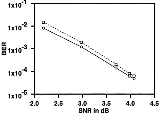
For example, on the BSC for a rate 2/3 encoder of 64 states (m = 6), the best previously known encoder is apparently a feed-forward encoder with [16]

15 15 6

G(D) = 153 136

2 13 13

We have found a feedback encoder with

L = , B(D)= 14 , N(D) 15 15 4 (4.1)

0 1 6 14 6 13 13

which performs better. At a crossover probability, p = 0.02, the feed-forward encoder had a BER = 1.496 x 10- 3, where our feedback code had a BER = 0.929 x 10-3.

.1

-2.

1x10--4

lx10-2

-, 1x10

- 3

--5

1x10-4

_x10-5 -. I I I I

2.0

2.5

3.0

3.5

4.0

4.5

SNR

in dB

Figure 4-1: Simulation results of rate 2/3 encoders with 64 states (m = 6) on the AWGN channel.

64 states (m = 6), the best previously known encoder is apparently a feed-forward encoder with

G(D) 15 6 17

6 15 15

The encoder with the best asymptotic performance bound on the AWGN channel is the same feedback encoder described in (4.1). The simulation results can be seen in Figure 4-1, where the dashed line represents the results of the feed-froward encoder and the solid line represents the results of our feedback encoder.

At a signal-to-noise ratio (SNR) of E = 4.07dB, the feed-forward encoder had a BER = 6.26 x 10- 5_{, where our feedback encoder had a BER = 4.69 x 10}- 5_{. The}

performance enhancement was even greater at low SNR. With -E

=

2.18dB, the feed-forward encoder had a BER = 1.48 x 10-2, while the feedback encoder had a BER

= 0.81 x 10-2. This improvement is approximately 0.225dB.

Appendix A

Corrections to [16]

In [16], Lobanov apparently overlooked the term i is his equation for the BER of a convolutional encoder over the BSC with low crossover probability p. The expression is given in Equation 2.2

Pb = -ABScPd + O(pd+1).

In Lobanov's paper, a factor of k should be found in the expected length of an error event

E(l(z)) = k(1 + O(p))

as p goes to zero for a rate k/n encoder. This overlooked term results in the error in the BER. We have not incorporated this factor into the constant ABSc so that our tables for rate 2/3 will agree with Lobanov's.

Also, there are two typos in Lobanov's table for rate 2/3 encoders. At m = 5 and

m = 7, the best codes listed by Lobanov do not perform as well as indicated. At

m = 5, Lobanov listed the code

7 4 7

G(D) =

3710

with an asymptotic coefficient ABSC = 109.75. We have calculated an asymptotic

coefficient for that code to be ABSC = 700.00. A simulation confirmed this result. A crossover probability p = 0.0142 led to a BER = 1.33 x 10- 3 _{for Lobanov's code. At}

m = 7, Lobanov's code

G(D)=

17 13 1

26 17

34

was listed with ABSC = 6374.03, where we have calculated As,,, = 12586.25 for the same code. Again, a simulation confirmed this result as a crossover probability p = 0.02 resulted in a BER = 1.51 x 10-3. Our calculations for ABSC were done using Lobanov's algorithm, and later verified using a brute force approach.

Appendix B

Corrections to [7]

I would like to point out a few typos in one of Dholakia's tables in [7]. Some rate 1/2 encoders in Table A.3 in [7] do not achieve the free distance listed, while other

turn out to be catastrophic. At m = 10, the encoder G(D) =

[

3413 2671

]

is

listed with a free distance df = 13. We have found the code to have a free distance

df = 11. Similarly, at m = 8, the encoder G(D) =

[

745 557] is listed with a free distance df = 11, while it achieves a free distance of df = 9. Also, at m = 7, the encoder G(D) = [367 361] is listed with free distance df = 9, while it obtains a

free distance df = 8. Furthermore, at m = 7, the encoder G(D) = [ 275 261

]

and

at m =4, the encoder G(D) = [35 27 are catastrophic.

Please note that Dholakia uses a different octal notation that we do, thus the code generators in his tables are not listed in the same form as ours.

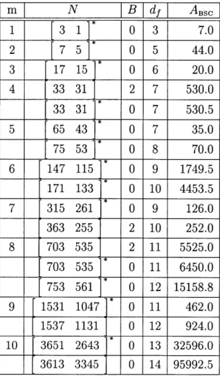
Appendix

C

mI

N

B

dfI

ABSC

1 3 1 0 3 7.0 2 7 5 0 5 44.0

3

17 15

0 6

20.0

4 33 31 2 7 530.0

33 31

0 7

530.5

5

65 43

0 7

35.0

75 53 0 8 70.0 6 147 115 0 9 1749.5 171 133 0 10 4453.5 7 315 261 0 9 126.0 363 255 2 10 252.0 8 703 535 2 11 5525.0 703 535 0 11 6450.0 753 561 0 12 15158.8 9 1531 1047 0 11 462.0 1537 1131 0 12 924.0 10 3651 2643 0 13 32596.0 3613 3345 0 14 95992.5

m

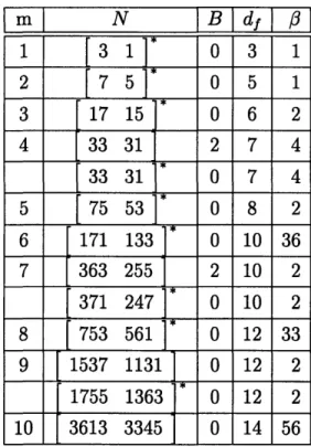
N

B df p]

1 3 1 0 3 1 2 7 5 0 5 1 3 17 15 0 6 2 4 33 31 2 7 4 33 31 0 7 4

5

75 53

0 8 2

6

171 133

0 10 36

7

363 255

2 10 2

371 247 0 10 2

8

753 561

0 12 33

9 1537 1131 0 12 2 1755 1363 0 12 2 10 3613 3345 0 14 56

Table C.2: Asymptotically good rate 1/2 encoders on the AWGN channel

m

N

B

Idf

ABsO

2 7 5 3 0 7 103.0 7 7 5 0 8 103.8 3 17 13 11 0 9 376.0 17 15 13 0 10 751.0 4 33 31 27 0 11 2766.0 37 33 25 0 12 5524.0 5 73 71 55 0 13 10290.0 6 157 135 123 2 15 77199.5 157 135 123 0 15 83639.0 7 367 331 225 0 16 6435.0 8 711 663 565 0 17 24310.0 727 623 575 0 18 48620.0

m

N

I

B

df

7]

2 7 7 5 0 8 3 3 17 15 13 0 10 6 4 37 33 25 0 12 12 5 75 53 47 0 13 1

6

157 135 123

2 15

6

175 155 123 0 15 7 7 367 331 225 0 16 1 8 727 623 575 0 18 2

Table C.4: Asymptotically good rate 1/3 encoders on the AWGN channel

m

N

B

L

Idf

ABss

123 22 10 2

₂₃

₃

₂₂

₁

₁

3 21.0 320 00 0 10 3 26.5 13 3 0 0 0 1 213 0 0 1 0 3 4 3.0 1 4 7 0 0 0 1 752 0 0 1 0 4 5 364.7 727 0 0 0 1 7 5 0 0 0 1 0 5 5 114.0 1 10 13 0 0 0 1 6 3 7 2 2 1 0 6 231.8 7 10 15 4 0 0 1 15 15 4 14 0 1 1 6 7 10706.9 6 1 13 3 6 14 0 1 15 15 6 0 0 1 0 7 13546.5 2 13 13 0 0 0 1 16 15 5 0 2 1 0 7 7 3085.0 11 20 27 0 2 0 1 13 7 12 0 0 1 0 7 3194.3 1 22 35 0 0 0 1 15 6 15 14 0 1 0 8 6697.6 13 23 24 12 2 0 1

m

N

B

L

edf

I

123 22 10 2

₂₃₃

₂

₂

₁₁

3 1

31 0

0

0

10

3

1

3 1 2 33 0 0 0 1 320 00 1

0

3 1 133 00 0 1 213 00 1 0 3 4 1 14 7 00 0 1 43 5 0 0 10 4 5 4 347 02 01 516 00 1 0 5 5 25 7 0 0 0 1 6 3 7 2 2 1 0 5 6 24 7 10 15 4 0 0 1 6 3 7 0 0 1 0 6 26 15 10 5 0 0 0 1 S 15 15 4 14 0 1 1 8 6 7 72 6 13 13 6 14 0 1 15 6 17 0 0 1 0 7 86 6 15 15 0 0 0 1 15 6 15 14 0 1 0 7 8 206 13 23 24 12 2 0 1 13 16 3 0 0 1 0 8 218 5 25 34 0 0 0 1

Appendix D

Im

N

iB

d~

Asc

1 3 1 0 3 7.0 2 7 5 0 5 44.0 3 17 15 0 6 20.0 4 33 31 2 7 530.0 33 31 0 7 530.5

35 23

0 7

548.0

5 65 43 0 7 35.0 75 53 0 8 70.0 75 55 0 8 207.5 73 55 0 8 245.0 6 147 115 0 9 1749.5 173 135 _ii- 0 9 2506.5 171 133 0 10 4453.5 147 135 0 10 5691.4

7

315 261

0 9

126.0

331 243 0 9 126.0

363 255

2 10

252.0

371 247 0 10 252.0 313 275 0 10 816.0 8 703 535 2 11 5525.0 703 535 0 11 6450.0 731 523 0 11 6460.5 753 561 0 12 15158.8 751 557 0 12 18402.5 9 1531 1047 0 11 462.0 1537 1131 0 12 924.0 1755 1363 0 12 924.0 10 3651 2643 0 13 32596.0 3745 2213 0 13 41168.0 3705 2227 0 13 42870.0 3613 3345 0 14 95992.5 3645 2671 0 14 140520.3

m

N

B df p

1 3 1 0 3 1 2 7 5 0 5 1 3 17 15 0 6 2 4 33 31 2 7 4

33 31

0 7

4

35 23 0 7 4 5 75 53 0 8 2

73 55

0 8

5

75 55 0 8 6 65 43 0 7 1

6

171 133

0 10 36

147 135

0 10 46

147 115 0 9 4

173 135

0 9

4

7

363 255

2 10

2

371 247 0 10 2 313 275 0 10 6 315 261 0 9 1 331 243 0 9 1 8 753 561 0 12 33 751 557 0 12 40

703 535

2

11

4

703 535 0 11 4

731 523

0 11

4

9 1537 1131

0 12 2

1755 1363 0 12 2

1531

1047

0 11

1

10

3613 3345

0 14 56

3645 2671 0 14 82 3745 2213 0 13 4 3651 2643 0 13 7 3705 2227 0 13 7

Im

N

B d

ABso

2 7 5 3 0 7 103.0 7 7 5 0 8 103.8 3 17 13 11 0 9 376.0 17 15 13 0 10 751.0 4 33 31 27 0 11 2766.0 37 33 25 0 12 5524.0 5 73 71 55 0 13 10290.0 75 53 47 0 13 15435.5 6 157 135 123 2 15 77199.5 157 135 123 0 15 83639.0

175 155 123

0 15 147945.5

175 145 133

0 15 173701.5

7 367 331 225 0 16 6435.0 8 711 663 565 0 17 24310.0 727 623 575 0 18 48620.0

711 663 557

0 18 267394.5

m

N

B dfl p

2 7 7 5 0 8 3 7 5 3 0 7 1

3

17 15 13

0 10

6

17 13 11 0 9 1

4

37

33

25

0 12 12

33 31 27

0 11 4

5

75 53 47

0 13

1

73 71 55

0 13

4

6

157 135 123

2 15

6

175 155 123 0 15 7 157 135 123 0 15 9 175 145 133 0 15 11 7 367 331 225 0 16 1

8

727 623

575

0 18

2

711 663 557 0 18 11

711 663 565

0 17

1

m N B L df ABSC

123

2 2

10

2 3 21.0 233 22 11 320 00 10 3 26.5 3 1 0 0 0 1 0 3 26.5 233 00 01 3 1 0 0 0 1 0 3 27.0 310 0 0 10 _{3 27.0} 123 20 01

2

13

0

0

10

3

27.5

3 27.5 103 0 0 01

213

0 0

10

_{3 37.5}

121

0

0

0

1

313 0 0 10 3 46.2 122 0 0 01 213 0 0 1 0 3 4 3.0 147 0 0 01 752 0 0 10 4 5 364.7 727 0 0 01 714 0 0 1 0 5 409.6 257 0 0 01 516 0 0 1 0 5 432.9 257 0 0 01 435 0 0 10 5 516.5 347 02 01 7 5 0 0 0 1 0 5 5 114.0 1 10 13 0 0 0 1 6 3 7 2 2 1 0 231.8 6 231.8 7 10 15 4 0 0 1 6 7 3 0 6 1 0 _{6 231.8} 1 12 13 0 12 0 1 6 3 7 0 0 1 247.8 6 247.8 15 10 5 0 0 0 1 6 3 7 0 0 1 0 6 331.2 3 10 17 0 0 0 1 7 4 7 0 0 1 0 5 700.0 3710 0 0 0 1

m

N

B

L

df

ABsc

15 15 4 14 0 1 1 6 7 10706.9 6 13 13 6 14 0 1 15 6 17 0 6 1 0 7 11098.9 6 15 15 0 14 0 1

15 15

6

0 0

1 0

7 13546.5

2 13 13

0 0

0 1

15 15

4

0 0

1 0

7 13563.5 6 13 13 0 0 0 1 15 6 17 0 0 1 0 7 13845.9 6 15 15 0 0 0 1 16 15 5 0 2 1 0 7 7 3085.0 11 20 27 0 2 0 1 13 7 12 0 0 1 0 7 3194.3 1 22 35 0 0 0 1 15 6 15 14 0 1 0 8 6697.6 13 23 24 12 2 0 1 13 6 13 12 0 1 0 8 6701.1 7 23 30 14 2 0 1 13 16 3 0 0 1 0 8 7125.6 5 25 34 0 0 0 1 14 7 13 0 0 1 0 8 8611.0

7 23 36

0 0

0 1

17 13 1

00

O

1

8 12586.3 26 17 34 0 0 0 1

m

N

B

L

df3

123 22 10 2 3 1 233 22 11 310 00 10 3 1 123 20 01 310 00 10 3 1 3 1 213 00 10 213 00 10 _{3 3} 121 0 0 01 313 00 10 3 4 12 2 0 0 1 213 0 1 0 3 5 103 00 01 21 3 0 0 1 0 3 4 1 14 7 0 0 0 1 S435 00 1 0 4 5 4 347 02 0 1 516 00 1 0 5 5 2 57 0 0 0 1 752 00 10 5 6 715 10 57 0 0 0 1

714

00

10

6 36

5 6 257 00 01 6 3 7 2 2 1 0 5 6 24

7 10

15

4

0

0

1

6 7 3 0 6 1 0 6 26 1 12 13 0 12 0 1 6 3 7 0 0 1 0 6 26 15 10 5 00 0 1 6 3 7 0 0 1 0 6 36 3 1017 0 0 0 1

7Table5 D.7: Rate 2/3 on the AWGN channel1encoders

5 2 1 10 13 00 0 1

7 4 7 0 0 1 0

5 24

3710 00 01

m

N

B

L

df

1

15 15 4 14 0 1 1 6 7 72 6 13 13 6 14 0 1 15 6 17 0 6 1 0 7 72 6 15 15 0 14 0 1 15 6 17 0 0 1 0 7 86 6 15 15 0 0 0 1 15 15 6 0 0 1 0 7 89 2 13 13 0 0 0 1 15 15 4 0 0 1 0 7 89 6 13 13 0 0 0 1 15 6 15 14 0 1 0 7 8 206 13 23 24 12 2 0 1 13 6 13 12 0 1 0 8 206 7 23 30 14 2 0 1 13 16 3 0 0 1 0 8 218 5 25 34 0 0 0 1 14 7 13 0 0 1 0 8 265

7 23 36

0 0

0 1

17 13 1 0 0 1 0 8 395 26 17 34 0 0 0 1 16 15 5 0 2 1 0 7 22 11 20 27 0 2 0 1 13 7 12 0 0 1 0 7 22 1 22 35 0 0 0 1

Bibliography

[1] M.R. Best, M.V. Burnashev, Y. Levy, A. Rabinovitch, P.C. Fishburn, A.R. Calderbank, and D.J. Costello. On a technique to caculate the exact perfor-mance of a convolutional code. IEEE Trans. on Inform. Theory, 41(2):441-447, March 1995.

[2] R.E. Blahut. Theory and Practice of Data Transmission Codes, Second Edition. Richard E. Blahut, 1996.

[3] M.V. Burnashev and D.L. Cohn. Symbol error probability for convolutional codes. _{Problemy Pereda6i Informacii (Problems of Inform. Transmission),} 26(4):3-15, 1990.

[4] M. Cedervall and R. Johannesson. A fast algorithm for computing distance spectrum of convolutional codes. IEEE Trans. on Inform. Theory, 35(6):1146-1159, Nov. 1989.

[5] J. Conan. The weight spectra of some short low-rate convolutional codes. IEEE

Trans. on Commun., 32(9):1050-1053, Sept. 1984.

[6] D.J. Costello. Construction of Convolutional Codes for Sequential Decoding. PhD

thesis, University of Notre Dame, 1969.

[7] A. Dholakia. Introduction to convolutional codes with applications. Kluwer Aca-demic Publishers, 1994.

[8] G.D. Forney. Convolutional codes i: algebraic structure. IEEE Trans. on Inform.

[9] G.D. Forney. Lower bounds on error probability in the presence of large inter-symbol interference. IEEE Trans. on Commun., 20(1):76-77, Feb. 1972.

[10] G.D. Forney. Maximum likelihood sequence estimation of digital sequences in the presence of intersymbol interference. IEEE Trans. on Inform. Theory, 18(3):363-378, May 1972.

[11] D. Haccoun and G. Begin. High-rate punctured convolutional codes for Viterbi and sequential decoding. IEEE Trans. on Commun., 37(11):1113-1125, Nov. 1989.

[12] R. Johannesson and E. Paaske. Further results on binary convolutional codes with an optimum distance profile. IEEE Trans. on Inform. Theory,

24(2):264-268, March 1978.

[13] T. Kailath. Linear Systems. Prentice-Hall, 1980.

[14] M. Kim. On systematic punctured convolutional codes. IEEE Trans. on

Com-mun., 45(2):133-139, Feb. 1997.

[15] K.J. Larsen. Short convolutional codes with maximal free distance for rates 1/2, 1/3, and 1/4. IEEE Trans. on Inform. Theory, 19(3):371-372, May 1973. [16] Yu. P. Lobanov. Asymptotic bit error probability for convolutional codes.

Problemy Peredadi Informacii (Problems of Inform. Transmission), 27(3):89-94,

1991.

[17] J.L. Massey and M.K.Sain. Inverses of linear sequential circuits. IEEE Trans.

on Computers, 17:330-337, 1968.

[18] J.E. Mazo. Faster-than-nyquist signaling. Bell Syst. Tech. J., 54:1451-1462, Oct. 1975.

[19] J.P. Odenwalder. Optimal decoding of convolutional codes. PhD thesis, University of California at Los Angeles, 1970.

[20] E. Paaske. Short binary convolutional codes with maximal free distance for rates 2/3 and 3/4. IEEE Trans. on Inform. Theory, 20(5):683-689, Sept. 1974. [21] C.E. Shannon. A mathematical theory of communication. Bell Systems Tech.

Journal, 27:379-423, 623-656, 1948.

[22] A.J. Viterbi and J.K. Omura. Principles of Digital Communication and Coding. McGraw-Hill, 1979.