DOI 10.1007/s10237-011-0320-4 O R I G I NA L PA P E R
3D characterization of bone strains in the rat tibia loading model
Antonia Torcasio · Xiaolei Zhang · Joke Duyck ·G. Harry van Lenthe
Received: 21 December 2010 / Accepted: 28 May 2011 / Published online: 18 June 2011 © Springer-Verlag 2011
Abstract Bone strain is considered one of the factors
inducing bone tissue response to loading. Nevertheless, where animal studies can provide detailed data on bone response, they only offer limited information on experimental bone strains. Including micro-CT-based finite element (micro FE) models in the analysis represents a potent methodology for quantifying strains in bone. Therefore, the main objective of this study was to develop and validate specimen-specific micro FE models for the assessment of bone strains in the rat tibia compression model. Eight rat limbs were subjected to axial compression loading; strain at the medio-proximal site of the tibiae was measured by means of strain gauges. Spec-imen-specific micro FE models were created and analyzed. Repeated measurements on each limb indicated that the effect of limb positioning was small (COV = 6.45 ± 2.27%). Instead, the difference in the measured strains between the animals was high (54.2%). The computational strains calcu-lated at the strain gauge site highly correcalcu-lated to the measured strains (R2 = 0.95). Maximum peak strains calculated at exactly 25% of the tibia length for all specimens were equal to 435.11 ± 77.88 microstrains (COV = 17.19%). In con-clusion, we showed that strain gauge measurements are very sensitive to the exact strain gauge location on the bone; hence,
A. Torcasio· G. H. van Lenthe (
B
)Division of Biomechanics and Engineering Design, Department of Mechanical Engineering, K.U.Leuven, Celestijnenlaan 300, 3001 Leuven, Belgium
e-mail: [email protected] X. Zhang· J. Duyck
BIOMAT, Department of Prosthetic Dentistry, K.U.Leuven, Kapucijnenvoer 7, 3000 Leuven, Belgium
G. H. van Lenthe
Institute for Biomechanics, ETH Zurich, Wolfgang-Pauli-Strasse 10, 8093 Zurich, Switzerland
the use of strain gauge data only is not recommended for stud-ies that address at identifying reliable relationships between tissue response and local strains. Instead, specimen-specific micro FE models of rat tibiae provide accurate estimates of tissue-level strains.
Keywords Tissue-level strains· Micro-CT · Voxel-based finite element models· Rat tibia compression loading · Strain gauge measurements
1 Introduction
Bone is a mechanosensitive tissue as it adapts its mass, archi-tecture, and mechanical properties in response to mechani-cal loading (Frost 2003). The beneficial effect of mechanical loading on bones has been the subject of a number of in vivo animal studies in which specific loading or unloading has been applied and the remodeling response evaluated. Well-known examples are the isolated avian ulna model (Rubin and Lanyon 1984), the rat tibiae bending (Turner et al. 1994) and the rat ulnar compression (Hsieh et al. 2001) model. Nevertheless, where animal studies provided detailed data on bone response, they were lacking a precise quantitative understanding of the local mechanical response. In most cases, strain levels in bone were estimated by strain gauge measurements only (Hsieh et al. 1999,2001;Kuruvilla et al. 2008; LaMothe et al. 2005; LaMothe and Zernicke 2004;
Robling and Turner 2002; Schriefer et al. 2005b; Uthge-nannt and Silva 2007;Xie et al. 2006;Zhang et al. 2006). In rodents, the small size of the bones dictated that only one single uniaxial gauge could be used, implicating that strain could only be measured locally and in one direction. As the strain field across the bone surface is not constant, it is likely that strain data were dependent on strain gauge placement.
Strain gauge placement is limited to certain locations because of size and accessibility issues as well as of the specific geom-etry of the bone tissue under investigation. This might explain the relatively large interindividual differences that have been reported in several studies (Hsieh et al. 1999,2001;Kuruvilla et al. 2008; Uthgenannt and Silva 2007). Micro-computed tomography (μCT) based finite element analysis appear to be a promising tool to quantify the strain field throughout the entire bone. Over the last years, μCT-based analysis has become a well-established technique for analyzing the mechanical competence of small trabecular bone samples (van Rietbergen et al. 1995). After nondestructive, three-dimensionalμCT scanning of the bone under investigation typically, a voxel-to-element conversion approach is used to create aμ-FE model that represents the bone structure in detail. This method is fast and can be completely automated. The voxel-based models, generally, comprise of a large num-ber of elements and typically require dedicated large-scale FE solvers (Adams 2002;Arbenz et al. 2008;Boyd et al. 2002;
van Rietbergen et al. 1995). With the increasing availabil-ity of parallel computers and dedicated solvers,μCT-based finite element analysis of whole bones or large portions can now be used as a high-throughput technique (van Lenthe et al. 2004,2008).
The aim of this study was to develop and validateμFE models for the assessment of tissue strain in a rat bone. Spe-cifically, the investigations were performed on the rat tibia compression model.
2 Materials and methods
Experiments were performed using 8 male Wistar rats (Janvier, France). All rats were 12 weeks old and weighted
257.1 ± 9.7g. The hind limbs of the rats were excised from
the middle of the femur to the toes and kept frozen at a tem-perature of−21◦C until the experimental testing. All proce-dures were approved by the ethical committee of K.U.Leuven (P029/2008).
2.1 Strain gauge measurements
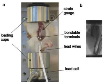
The limbs were thawed 12 h prior to the experiments. Inci-sions were made through the skin, and muscles were retracted to expose the medio-proximal surface of the bones. The bonding surface of the specimens was lightly polished with an abrasive paper and wiped with acetone. For each speci-men, a single element strain gauge (type FLG-02-11, TML, Tokyo Sokki Kenkyujo Co., Ltd.) with an active gauge length of 0.2 mm and width of 1.4 mm was used. The strain gauge was glued using a cyanoacrylate adhesive (type CN, Feteris Components BV) on the medial surface of the tibia at 25% of the tibia length (Fig.1a). The lead wires (type 3WP008,
Fig. 1 Rat limbs were placed between the loading cups connected to the BOSE test bench (a). A rat limb is constrained by two plastic cups for further imaging byμCT (b)
Feteris Components BV) were connected on one end to the delicate jumper wires of the strain gauge through bond-able terminals (TF-2SS, Feteris Components BV) that were attached on the bone surface below the strain gauge. On the other end, the lead wires were connected to the acquisition system. The limbs were placed between two dedicated load-ing cups of a testload-ing system (BOSE TestBench LM1, Endura-TEC Systems Group, Bose Corp., Minnetonka, MN, USA) and kept in place by means of a 0.5 N preload. After 4 condi-tioning cycles, strain was measured at compressive forces of 2.5, 5.0, 7.5, and 10.0 N, respectively, at a rate of 0.5 mm/sec. The strain reading system included the acquisition of the signal after quarter bridge (SCXI 1314, NI, National Instru-ments, Austin, TX), amplification, and conditioning (SCXI 1520, NI) and the transmission to the PC (SCXI 1600 USB DAQ module, NI). Labview software (Labview 8.6, NI) pro-vided the necessary interface and readout. To quantify the potential strain variations due to leg orientation, measure-ments were repeated 5 times after complete removal of the specimen from the device followed by repositioning.
2.2μCT imaging
Before the experiment, the excised limbs had been imaged by
μCT (Skyscan 1172, Skyscan, Kontich, Belgium) from the
knee to the ankle joint while being constrained by two plastic cups as in the experimental configuration (Fig.1b). Because of the large size of the specimens, we adopted the “oversize scan” modality that can image sequentially at high resolu-tion and connect together multiple views along the height of the specimens. The number of subscans was equal to 6 for all specimens. Each subscan was taken with 20µm reso-lution, 70 kV source voltage, 141µA source current, 2-fold oversampling, and a rotation step of 0.350 degrees.
After the experiments, all samples with the strain gauges still bonded to the bone surface were imaged again byμCT. 2.3 Micro-CT-based finite element analysis (μFE)
The images were reconstructed using the Skyscan NRec-on software (versiNRec-on 1.6.1.5) that performed automatic matching and connections of the parts belonging to each oversize scan without inducing any misalignment artifact in the structure. The quality of the post-experimentμCTs was limited due to the presence of metal artifacts in proximity of the jumper wires of the strain gauges.
Both pre and post-experimentμCT scans of each spec-imen were processed (IPL, Scanco Medical, Brüttisellen, Switzerland). To reduce computational costs, the voxel size was set to 40μm. The μCT images of each tibia were fil-tered using a constrained three-dimensional Gaussian filter to partially suppress the noise in the volumes (σ = 1.2, support= 2).
The data were binarized using a global threshold of 14% of maximum possible gray value, for which the extracted bone represented well the actual structure (Bouxsein et al. 2010). The joint spaces between the articulating bones of the system (tibia-femur, femur-patella, tibia-talus, talus-cal-caneus) were filled with connection elements. Finally, a com-ponent labeling algorithm was applied in order to delete all the unconnected elements in the model.
The models based on the artifact-free preexperimental images were analyzed. Micro-finite element (μFE) models were generated for each tibia by a direct conversion of bone voxels to linear hexahedral elements. Voxel size was 40µm. Mesh convergence tests were performed on one sample by calculating the overall sample stiffness when using voxel sizes of 20, 40, and 80µm, respectively (data not shown). For the 80µm voxels, the difference relative to the model with 20µm voxels was 1.35%, while it was 1.30% for the 40µm voxels. Accordingly, it was concluded that the 40µm voxel mesh was sufficiently converged.
All elements in theμFE models were given an arbitrary tissue modulus of 10 GPa and a Poisson ratio of 0.3. Bound-ary conditions that simulated the experimental configuration were defined. Hence, the models were fixed at the distal end; to the top nodes an axial displacement that resulted in 0.1% overall strain was applied, while any displacement in the other two directions was constrained. The models were solved using the dedicated large-scale finite element solver ParFE (Arbenz et al. 2008) using 256 cores on a Cray XT5 system.
2.4 Calculation of the strains at the strain gauge site Fully automated alignment routines of the post-experimental model onto the preexperimental artifact-free model were
performed, which allowed for identifying the location of the strain gauge with respect to each tibia model; hence, a vol-ume of interest VOI identifying the strain gauge location was selected.
In order to prevent artificial surface strain values from affecting the results, the surface layer of the VOI was excluded from the analysis; artificial surface strains can arise because of the voxel-based nature of the micro-FE models.
For each element, the strains tensor was calculated and averaged over the VOI. Three-dimensional strain transforma-tions were applied to obtain the strain in the working direc-tion of the experimental strain gauge. In order to allow the comparison with the experimental strains engendered by the maximum applied load, strain element data corresponding to 9.5 N load magnitude (=10.0 – 0.5 N preload) were deter-mined on the basis of the calculated reaction force. Bone tis-sue modulus was calculated as the tistis-sue modulus for which the averaged micro-FE calculated strain was identical to the averaged measured strains (van Lenthe et al. 2008). Visu-alizations of the bone strains were created using the open source program ParaView (http://www.paraview.org/), run-ning on an HP-XC cluster.
2.5 Effect of strain gauge placement
We examined the strain distribution of the cross-section taken at the level of the strain gauge site. Second, we analyzed the sensitivity of the FE results to strain gauge placement. Spe-cifically, we evaluated the effect of small changes in strain gauge location (∼±0.5mm) along the anterior-posterior and the proximal-distal axes. Furthermore, we calculated the sen-sitivity of the results to changes in gauge alignment (5◦and 10◦on each side of longitudinal alignment).
Finally, we extracted a 0.2 mm thick subvolume (5 slices) at exactly 25% of the tibia length for all specimens of which we calculated minimum and maximum cross-sectional peak strain values.
In order to evaluate to which extent bone cross-sectional geometry contributed to the interindividual differences in tissue-level strains, we included measures that can be deter-mined from a cross-sectional image; more precisely, area (Ar; mm2), and maximum and minimum moment of area (Imax, Imin; mm4) were calculated for each slice and aver-aged over the 0.2 mm thick subvolume.
2.6 Statistical analysis
For each load magnitude, mean strains and standard devi-ations over 5 repeated measurements were calculated. The intra-individual variability assessed in terms of coefficient of variation (COV). The experimental interindividual vari-ability was calculated based on the slopes of the relation-ships between mean strains and load magnitude of the eight
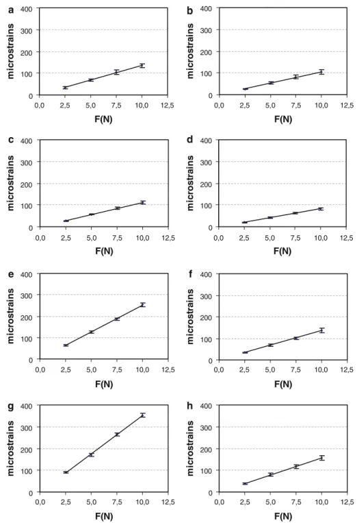
Fig. 2 Experimentally measured strain—force relationship for the 8 limbs tested (a–h). Each value represents the mean strain and standard deviation over 5 repeated measurements performed on the same limb using the same strain gauge
0 100 200 300 400 F(N) m icr o s tr ai n s 0 100 200 300 400 F(N) m icr o s tr ai n s 0 100 200 300 400 0,0 2,5 5,0 7,5 10,0 12,5 F(N) m icr o s tr ai n s 0 100 200 300 400 F(N) m icr o s tr ai n s b 0 100 200 300 400 F(N) m icr o s tr ai n s 0 100 200 300 400 F(N) m icr o s tr ai n s 0 100 200 300 400 F(N) mic ro s tr a in s 0 100 200 300 400 F(N) m icr o s tr ai n s c a d e f g h 0,0 2,5 5,0 7,5 10,0 12,5 0,0 2,5 5,0 7,5 10,0 12,5 0,0 2,5 5,0 7,5 10,0 12,5 0,0 2,5 5,0 7,5 10,0 12,5 0,0 2,5 5,0 7,5 10,0 12,5 0,0 2,5 5,0 7,5 10,0 12,5 0,0 2,5 5,0 7,5 10,0 12,5
limbs. The experimental mean strains were correlated to the computational strains by means of the Pearson’s squared correlation coefficient (R2). As an indicator of the differ-ence between numerical and experimental strains, the root mean-square error (RMSE) and the prediction error were calculated; both values were also expressed as a percent-age by normalizing the absolute values by the mean of the experimentally measured strains. The effective interindivid-ual variability was assessed in terms of the coefficient of variation in the peak strain magnitudes calculated over the subvolume extracted at 25% of the tibia length. Pearson’s
correlation coefficients (r ) between peak strain magnitude and structural parameters were determined. All statistical analysis were performed with Excel 2003 (Microsoft, Red-mond, USA).
3 Results
3.1 Strain gauge measurements
Compressive loading of the rat limbs resulted in tensile strains on the medio-proximal surface of the tibia. The
y = 1.20x - 32.59 R2 = 0.95 0 100 200 300 400 500 0 100 200 300 400 500
computational strains with E = 18.281 GPa (microstrains)
experimental strains
(microstrains)
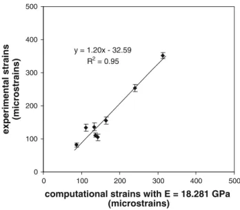
Fig. 3 Experimentally measured strains versus computational strains calculated at 9.5 N load amplitude and a tissue modulus of 18.3 GPa
measured strains differed by 54.2% between individuals. However, intra-individual variability was as low to 6.45 ±
2.27%.
Over the range of load magnitudes applied, we found for each limb that the mean strains exhibited a linear relation to the applied loads (Fig.2).
3.2 Validation of theμFE models
In total, eightμFE models were analyzed, one model for each bone. On average, theμFE models consisted of 7.9 million elements and 9 million nodes, respectively. EachμFE model was solved in approximately 9 minutes.
The strains as calculated by theμFE models correlated highly (R2 = 0.95) to the strains measured at 9.5N com-pression load (Fig.3); RMSE was found to be 23.5 micro-strains (14.1%); the prediction error was 13.6 micromicro-strains (8.2%). In absolute values, the computational strains closely matched the experimental strains when a tissue modulus of 18.3 GPa was assumed.
3.3μFE models versus strain gauge measurements
The visualization of the strain distribution demonstrated that axial loading produced a mixture of compression and bending, which resulted in tensile and compressive strains on the medial and lateral surface of the proximal tibia, respec-tively (Fig.4a).
The strain distribution at the level of the strain gauge site indicated that peak tensile strains were located at the anterior side of the tibia and were equal to 413.68 ± 70.86 micro-strains (Fig.4b). The coefficient of variation was 17.13%.
a b
ε33_max
ε33_min
0 Strain gauge site
+
Fig. 4 Strain distribution throughout the whole rat tibia loading model. Tensile (blue) and compressive (red) strains are occurring in the prox-imal tibia on the medial and lateral side, respectively (a). Strain dis-tribution in the cross section at the location of the strain gauge site. The sign convention for the angles of gauge alignment is indicated: a positive angle with respect to the longitudinal axis of the tibia refers to a clockwise rotation of the VOI around the y axis (b)
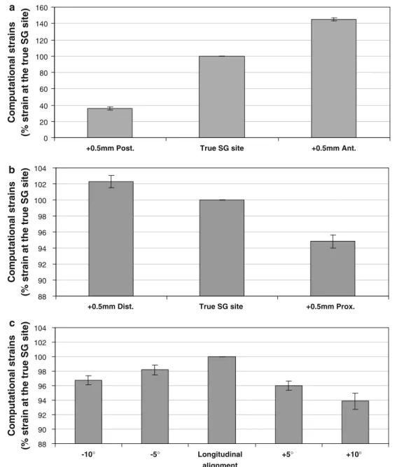
Changes in strain gauge location of 0.5 mm toward the anterior and posterior side of the tibiae induced, on average, strain differences of +45.07% and −64.31% with respect to the true strain gauge site, respectively. Changes in gauge location toward the proximal and distal side induced strain differences of−5.39% and 2.38%, respectively. The change in strain gauge alignment by 10◦ and 5◦, −5◦ and −10◦ (Fig. 4b) with respect to perfect longitudinal alignment caused, on average strain differences equal to −6.03%, −3.99%, −1.72%, and −3.29%, respectively. Maximum cross-sectional peak strain in the subvolume selected at 25% of the tibia length was equal to 435.11 ± 77.88 micro-strains. Minimum cross-sectional peak strain was equal to −533.02 ± 86.01 microstrains. The coefficients of variation were equal to 17.19% and 16.14% for maximum and mini-mum strains, respectively.
The maximum moment of area Imax correlated with the maximum longitudinal strain (r = −0.84) as well as with the minimum longitudinal strain (r = −0.84). Similar find-ings were found for the minimum moment of area Imin, which correlated to the maximum (r = −0.79) and mini-mum (r = −0.82) longitudinal strains and for the cross-sec-tional area Ar (r = −0.65 and r = −0.69, respectively).
The interindividual COV in Imax, Imin and Ar was 13.6%, 18.0%, and 10.3%, respectively.
4 Discussion
The main objective of this study was to develop and validate specimen-specificμFE models for the assessment of tissue strain in the rat tibia compression model.
The entire rat limbs were modeled, and an eventual in vivo experiment was simulated. Whereas leg orientation only moderately affected bone strains in a four-point bending model of rat tibiae (Akhter et al. 1992), very strong effects of bone orientation were found in an axial loading model of murine femora (Voide et al. 2008). By using dedicated load-ing cups, we aimed in havload-ing a reproducible limb orientation. Our results proved that we succeeded because repeated mea-surements on each specimen showed high precision(COV =
6.45 ± 2.27%), indicating that this effect was small.
We found that the computational strains calculated at the strain gauge site highly correlated to the measured strains (R2 = 0.95). We calculated that a tissue modulus of 18.3 GPa provided the best match between experimental and com-putational strain data. A previous study (Huang et al. 2003) had reported a lower value of tissue modulus (13.8 GPa) for Wistar rat tibiae. This lower value is likely to be related to the fact that in their study the tissue modulus had been quantified by three-point bending testing in combination with beam the-ory, and it is well known that this method may cause a strong underestimation of Young’s modulus (Schriefer et al. 2005a;
Torcasio et al. 2008;van Lenthe et al. 2008). It is also possi-ble that the tibiae were less stiff compared to the tibiae tested in our studies because the bones were derived from younger animals (7 weeks versus 12 weeks of age, respectively).
We found relatively large COV for the experimentally measured interindividual strains, for which we identified three potential sources of error related to the strain gauge placement. First, the strain gauge had been placed in a region characterized by high strain gradients along the anterior– posterior direction. We demonstrated that a small differ-ence in the strain gauge location along the anterior–posterior direction would induce a large difference in strain readings (−64.31% and 45.07% at 0.5mm from the strain gauge site toward the anterior and posterior side of the tibiae, respec-tively). Second, the μCT images revealed that the strain gauges also slightly varied in their longitudinal position. We demonstrated that a variation of 0.5 mm toward the proximal and distal side could induce a difference in measured strains by−5.39% and 2.38%, respectively. Third, the strain gauge may not have been perfectly aligned in all specimens. We calculated an underestimation of up to 6.03%, for alignment errors up to 10 degrees with respect to perfect longitudinal alignment (Fig.5).
These findings indicated strain gauge placement as a fun-damental source of variability in experimentally measured strains. As confirmation of that maximum tensile strains cal-culated at exactly 25% of the tibia, hence corresponding to same strain gauge location and alignment indicated an inter-individual difference of 17.9%, which is about 1/3 of the interindividual difference provided by the experimental mea-surements.
Apart from the strain gauge placement, the measurements might have been affected also by the variability in bone cross-sectional geometry. We found that the maximum moment of inertia, to which the peak strains correlated highly (r = −0.82), varied by 13.6% between individuals. Other causes which might have contributed to the interindividual differ-ence in measured strains are the bone tissue properties and soft tissue characteristics, which might vary between indi-viduals. In addition, a possible shifting of the joint alignment under the experimentally applied loads might have occurred, which affected the measurements.
In this study, we demonstrated relevant advantages of using the micro-CT-based finite element method to assess the strains in the rat tibia loading model. First, the use of voxel-based FE models allowed for a highly accurate repre-sentation of both the complex external shape and the inner microarchitecture of bone. The main advantage to incorpo-rate the microarchitecture into the FE models was that the anisotropy resulting from the trabecular bone microstructure was automatically taken into account (van Lenthe and Muller 2006). Second, as it is a critical factor for the assessment of tissue strain in the rat tibia, the loads had to be repre-sented accurately. Because of the complexity of the system, an analytical determination of the load transfer through the knee joint to the tibia was not possible. For this reason, each limb was imaged positioned between two cups as in the experimental configuration, such that the correct align-ment of model with respect to the loading direction and the point of load application were automatically incorporated in the specimen-specific reconstructed models. This provided major advantages over previously published studies in which micro-CT-based models of the bone (tibia, ulna) alone have been created and for which bone alignment with respect to the loading direction can be problematic (Chennimalai et al. 2010;Kotha et al. 2004;Stadelmann et al. 2009). Third, the
μFE models were not suffering from some of the
experimen-tal limitations such as the limited availability in good bony locations for strain gauge placement, nor in the limitations of placing the strain gauge at the correct position, nor in the assessment of strain in just one direction. Instead, theμFE models provided a complete three-dimensional quantifica-tion of the strains throughout the bone and in any direcquantifica-tion. One limitation of our approach consists in the approxima-tions introduced when modeling the ankle and the knee joints. We modeled the cartilage by elements that were as stiff as the
0 20 40 60 80 100 120 140 160
+0.5mm Post. True SG site +0.5mm Ant.
Computational strains
(% strain at the true SG site)
88 90 92 94 96 98 100 102 104 -10° -5° Longitudinal alignment +5° +10° Computational strains
(% strain at the true SG site)
88 90 92 94 96 98 100 102 104
+0.5mm Dist. True SG site +0.5mm Prox.
Computational strains
(% strain at the true SG site)
a
b
c
Fig. 5 Computationally calculated strains at 0.5 mm toward the ante-rior (‘+0.5 mm Ant.’) and posteante-rior side (‘+0.5 mm Post.’) of the tibiae with respect to the true strain gauge site (‘True SG site’) (a); compu-tationally calculated strains at 0.5 mm toward the proximal (‘+0.5 mm Prox.’) and distal side (‘+0.5 mm Dist.’) of the tibiae with respect to the
true strain gauge site (b); computationally calculated strains when the strain gauge alignment is changed by 10◦and 5◦, −5◦and−10◦with respect to perfect longitudinal alignment (c). The value at the true SG site was set to 100% for each bone
bone, and we assumed no relative motion between the bony segments. Nevertheless, this rather crude joint modeling approach allowed us to represent the bones as positioned in their experimental configuration such that the correct loading direction and point of load application were automatically incorporated into the finite element models. More impor-tantly, the very good agreement between experimental and computational strains indicated that this modeling approach was adequate.
In conclusion, we have demonstrated that μFE models can provide accurate estimates of tissue-level strains in rat tibia when exposed to controlled mechanical loading. We also demonstrated that the data obtained by strain gauge mea-surements are strongly affected by strain gauge placements. Combining experimental measurements with highly accurate specimen-specific finite element analysis can provide quan-titative and reliable strain data. We believe that these findings have important implications for studies on bone adaptation,
for which accurate relationships between local mechanical stimuli and local tissue response are mandatory.
Acknowledgments The authors acknowledge the Laboratory for Experimental Medicine and Endocrinology (LEGENDO) of Leuven for allowing the use of theμCT scanner and the Swiss National Supercom-puting Centre (CSCS) that granted the computational time. This study was supported by the grant OT/04/26 from the Katholieke Universiteit Leuven.
References
Adams M (2002) Evaluation of three unstructured multigrid methods on 3D finite element problems in solid mechanics. Int J Numer Meth Eng 55:519–534
Akhter MP, Raab DM, Turner CH, Kimmel DB, Recker RR (1992) Characterization of in vivo strain in the rat tibia during external application of a four-point bending load. J Biomech 25(10):1241– 1246
Arbenz P, van Lenthe GH, Mennel U, Müller R, Sala M (2008) A scal-able multi-level preconditioner for matrix-freeμ-finite element analysis of human bone structures. Int J Numer Meth Eng 73:927– 947
Bouxsein ML, Boyd SK, Christiansen BA, Guldberg RE, Jepsen KJ, Müller R (2010) Guidelines for assessment of bone microstruc-ture in Rodents using micro-computed tomography. J Bone Miner Res 25(7):1468–1486
Boyd SK, Muller R, Zernicke RF (2002) Mechanical and architectural bone adaptation in early stage experimental osteoarthritis. J Bone Miner Res 17(4):687–694
Chennimalai KN, Dantzig JA, Jasiuk IM, Robling AG, Turner CH (2010) Numerical modeling of long bone adaptation due to mechanical loading: correlation with experiments. Ann Biomed Eng 38(3):594–604
Frost HM (2003) Bone’s mechanostat: a 2003 update. Anat Rec A Dis-cov Mol Cell Evol Biol 275(2):1081–1101
Hsieh YF, Robling AG, Ambrosius WT, Burr DB, Turner CH (2001) Mechanical loading of diaphyseal bone in vivo: the strain threshold for an osteogenic response varies with location. J Bone Miner Res 16(12):2291–2297
Hsieh YF, Wang T, Turner CH (1999) Viscoelastic response of the rat loading model: implications for studies of strain-adaptive bone formation. Bone 25:379–382
Huang TH, Lin SC, Chang FL, Hsieh SS, Liu SH, Yang RS (2003) Effects of different exercise modes on mineralization, structure, and biomechanical properties of growing bone. J Appl Physiol 95(1):300–307
Kotha SP, Hsieh YF, Strigel RM, Muller R, Silva MJ (2004) Experi-mental and finite element analysis of the rat ulnar loading model-correlations between strain and bone formation following fatigue loading. J Biomech 37(4):541–548
Kuruvilla SJ, Fox SD, Cullen DM, Akhter MP (2008) Site specific bone adaptation response to mechanical loading. J Musculoskelet Neu-ronal Interact 8(1):71–78
LaMothe JM, Hamilton NH, Zernicke RF (2005) Strain rate influences periosteal adaptation in mature bone. Med Eng Phys 27:277–284 LaMothe JM, Zernicke RF (2004) Rest insertion combined with high-frequency loading enhances osteogenesis. J Appl Physiol 96: 1788–1793
Robling AG, Turner CH (2002) Mechanotransduction in bone: genetic effects on mechanosensitivity in mice. Bone 31(5):562–569 Rubin CT, Lanyon LE (1984) Regulation of bone formation by applied
dynamic loads. J Bone Joint Surg Am 66(3):397–402
Schriefer JL, Robling AG, Warden SJ, Fournier AJ, Mason JJ, Turner CH (2005a) A comparison of mechanical properties derived from multiple skeletal sites in mice. J Biomech 38(3):467–475 Schriefer JL, Warden SJ, Saxon LK, Robling AG, Turner CH
(2005b) Cellular accommodation and the response of bone to mechanical loading. J Biomech 38(9):1838–1845
Stadelmann VA, Hocke J, Verhelle J, Forster V, Merlini F, Terrier A, Pioletti DP (2009) 3D strain map of axially loaded mouse tibia: a numerical analysis validated by experimental measurements. Comput Methods Biomech Biomed Eng 12(1):95–100
Torcasio A, van Oosterwyck H, van Lenthe GH (2008) The system-atic errors in tissue modulus of murine bones when estimated from three-point bending. J Biomech 41:S14
Turner CH, Forwood MR, Otter MW (1994) Mechanotransduction in bone: do bone cells act as sensors of fluid flow. FASEB J 8(11):875–878
Uthgenannt BA, Silva MJ (2007) Use of the rat forelimb compression model to create discrete levels of bone damage in vivo. J Biomech 40(2):317–324
van Lenthe GH, Kohler T, Voide R, Donahue LR, Müller R (2004) Functional phenomics in bone: high-throughput assessment of genetic differences in murine inbred strains. J Bone Miner Res 19((1):S390
van Lenthe GH, Voide R, Boyd SK, Muller R (2008) Tissue modulus calculated from beam theory is biased by bone size and geometry: implications for the use of three-point bending tests to determine bone tissue modulus. Bone 43(4):717–723
van Lenthe GH, Muller R (2006) Prediction of failure load using micro-finite element analysis models: toward in vivo strength assessment. Drug Discov Today Technol 3:221–229
van Rietbergen B, Weinans H, Huiskes R, Odgaard A (1995) A new method to determine trabecular bone elastic properties and load-ing usload-ing micromechanical finite-element models. J Biomech 28(1):69–81
Voide R, van Lenthe GH, Muller R (2008) Femoral stiffness and strength critically depend on loading angle: a parametric study in a mouse-inbred strain. Biomed Tech (Berl) 53(3):122–129 Xie L, Jacobson JM, Choi ES, Busa B, Donahue LR, Miller LM, Rubin
CT, Judex S (2006) Low-level mechanical vibrations can influ-ence bone resorption and bone formation in the growing skeleton. Bone 39:1059–1066
Zhang P, Tanaka SM, Jiang H, Su M, Yokota H (2006) Diaphyseal bone formation in murine tibiae in response to knee loading. J Appl Physiol 100:1452–1459