Climate of the Last Glacial Maximum: sensitivity studies and model-data comparison with the LOVECLIM coupled model

HAL Id: hal-00298075

https://hal.archives-ouvertes.fr/hal-00298075

Submitted on 15 May 2007

HAL is a multi-disciplinary open access

archive for the deposit and dissemination of

sci-entific research documents, whether they are

pub-lished or not. The documents may come from

teaching and research institutions in France or

abroad, or from public or private research centers.

L’archive ouverte pluridisciplinaire HAL, est

destinée au dépôt et à la diffusion de documents

scientifiques de niveau recherche, publiés ou non,

émanant des établissements d’enseignement et de

recherche français ou étrangers, des laboratoires

publics ou privés.

studies and model-data comparison with the

LOVECLIM coupled model

D. M. Roche, T. M. Dokken, H. Goosse, H. Renssen, S. L. Weber

To cite this version:

D. M. Roche, T. M. Dokken, H. Goosse, H. Renssen, S. L. Weber. Climate of the Last Glacial

Max-imum: sensitivity studies and model-data comparison with the LOVECLIM coupled model. Climate

of the Past, European Geosciences Union (EGU), 2007, 3 (2), pp.205-224. �hal-00298075�

www.clim-past.net/3/205/2007/

© Author(s) 2007. This work is licensed under a Creative Commons License.

of the Past

Climate of the Last Glacial Maximum: sensitivity studies and

model-data comparison with the LOVECLIM coupled model

1_{Department of Palaeoclimatology and Geomorphology, Faculty of Earth and Life Sciences, Vrije Universiteit Amsterdam,} De Boelelaan 1085, 1081 HV Amsterdam, The Netherlands

2_{Bjerknes Center for Climate Research, Allegaten 55, 5007 Bergen, Norway}

3_{Institut d’Astronomie et de G´eophysique G. Lemaˆıtre. 2, Chemin du Cyclotron, 1348 Louvain-la-Neuve, Belgium} 4_{Royal Netherlands Meteorological Institute (KNMI), P.O. Box 201, 3730 AE De Bilt, The Netherlands}

Received: 9 October 2006 – Published in Clim. Past Discuss.: 8 November 2006 Revised: 21 February 2007 – Accepted: 3 May 2007 – Published: 15 May 2007

Abstract. The Last Glacial Maximum climate is one of the

classical benchmarks used both to test the ability of cou-pled models to simulate climates different from that of the present-day and to better understand the possible range of mechanisms that could be involved in future climate change. It also bears the advantage of being one of the most well documented periods with respect to palaeoclimatic records, allowing a thorough data-model comparison. We present here an ensemble of Last Glacial Maximum climate simu-lations obtained with the Earth System model LOVECLIM, including coupled dynamic atmosphere, ocean and vegeta-tion components. The climate obtained using standard pa-rameter values is then compared to available proxy data for the surface ocean, vegetation, oceanic circulation and atmo-spheric conditions. Interestingly, the oceanic circulation ob-tained resembles that of the present-day, but with increased overturning rates. As this result is in contradiction with the current palaeoceanographic view, we ran a range of sensitiv-ity experiments to explore the response of the model and the possibilities for other oceanic circulation states. After a crit-ical review of our LGM state with respect to available proxy data, we conclude that the oceanic circulation obtained is not inconsistent with ocean circulation proxy data, although the water characteristics (temperature, salinity) are not in full agreement with water mass proxy data. The consistency of the simulated state is further reinforced by the fact that the mean surface climate obtained is shown to be generally in agreement with the most recent reconstructions of vegetation and sea surface temperatures, even at regional scales.

Correspondence to: D. M. Roche

(didier.roche@falw.vu.nl)

1 Introduction

For climate modellers, the Last Glacial Maximum (LGM) is a standard period to evaluate their model’s capability to sim-ulate a climate that is drastically different from that of the present-day. These evaluations have been supported by sev-eral projects aimed at the reconstruction of the LGM surface conditions based on proxy data, like CLIMAP (CLIMAP, 1981), GLAMAP2000 (Sarnthein et al., 2003) and MARGO (Kucera et al., 2005a), providing strong constraints on what the climate looked like at that period of time. At the same time, efforts have been undertaken to improve inter-comparisons of the different models under glacial bound-ary conditions such as the pioneering work of the Palaeo-climate Modeling Intercomparison Project (PMIP). In its first phase PMIP applied Atmospheric General Circulation models (Joussaume and Taylor, 2000), followed by Coupled Atmospheric-Ocean models in its second phase (PMIP2) (see also website http://pmip2.lsce.ipsl.fr Crucifix et al., 2005; Braconnot et al., 2007). Comparisons between PMIP models were also conducted to evaluate the results against surface data of the LGM (Kageyama et al., 2001, 2006). Those com-parisons have shown that the inclusion of more components in the climate system have resulted in better agreement with the data (Kageyama et al., 2006). At the same time, some work on data assimilation of MARGO data in a simplified coupled model (Paul and Sch¨afer-Neth, 2005) has proven the significance of the mean surface climate in determining the consistency of the simulated climate with respect to data.

However, there is still strong disagreement between mod-els with respect to one of the major components of the cli-mate system: the oceanic thermohaline circulation (THC). In the few LGM experiments conducted with coupled Atmosphere–Ocean models (Kitoh et al., 2001; Hewitt et al., 2003; Shin et al., 2003; Kim, 2004) the strength of the

thermohaline circulation and the relative importance of the different water masses differs considerably. Mechanisms un-derlying the simulated THC response were found to differ widely in an inter-comparison study of PMIP coupled model simulations (Weber et al., 2007). The current palaeoceano-graphic interpretation of data is a weaker overturning, with a shallower North Atlantic water mass and a denser and more predominant Antarctic water mass. However, some uncer-tainties remain on the precise relationships between the water masses.

In this study, we present an extensive comparison between our simulated LGM climate and available data to evaluate the agreement between the two. We consider both the sur-face climate and the deep ocean circulation. We have also performed a suite of sensitivity experiments to study the re-sponse of the glacial ocean circulation to different model pa-rameters. The aim is to assess how different setups may yield different types of global meridional circulation.

A precise definition of the LGM is required. Although it originally refers to the maximum of globally averaged con-tinental ice that occurred during the last glacial period, it is usually difficult to derive that period from a given data archive. Thus, the period taken depends on the archive (Sarn-thein et al., 2003, for example). In this paper, we will further refer to the LGM as the period around 21 thousand years be-fore present (kyrs B.P.), coherent with the commonly used time period in previous climate simulations and being also the centre of the period used in most recent reconstructions (Kucera et al., 2005a).

2 The LOVECLIM model and the LGM

2.1 Model description

In this study we use the three-dimensional Earth System model LOVECLIM. LOVECLIM is an acronym made from the names of the five different models that have been cou-pled to build the Earth system model: LOch–Vecode–Ecbilt– CLio–agIsm Model (LOVECLIM, Driesschaert, 2005). Here only the atmosphere–ocean–vegetation part is used (ECBilt– CLIO–VECODE). Actually, in the configuration chosen here, the model gives exactly the same results as ECBilt-CLIO-VECODE version 3, used for instance by Goosse et al. (2005) and Renssen et al. (2005) to study the climate of the past millennium and of the Holocene respectively (but is sub-stantially different from the one used by Timmermann and Goosse, 2004). Nevertheless, many technical changes have been included in the code recently, in particular in order to allow for the coupling with ice sheet and carbon cycle mod-els. As a consequence, for simplicity, users and developers have decided jointly that the new name LOVECLIM should now be used for the model, even if some components are not activated (see http://www.astr.ucl.ac.be/index.php?page= LOVECLIM@SumLove).

The atmospheric model is a global quasi-geostrophic, spectral model at T21 horizontal resolution, with additional parameterisations for the diabatic heating due to radiative fluxes, the release of latent heat, and the exchange of sen-sible heat with the surface (Opsteegh et al., 1998). The ocean part is a three dimensional, free surface, general cir-culation model coupled to a thermodynamical and dynami-cal sea-ice model (Goosse and Fichefet, 1999). The vege-tation part is the VECODE dynamical terrestrial vegevege-tation model (Brovkin et al., 1997) which computes plant fractions for trees and herbaceous (plus desert) from several atmo-spheric variables in each land grid-cell. To easily compare the output of VECODE with available vegetation reconstruc-tions for the LGM, we developed a module to assign biomes from the Plan Functional Types (PFTs) computed by the veg-etation model (see Sect. 2.3).

As such, the Earth system model used here is able to sim-ulate the climate with some details while still being compu-tationally efficient, and therefore allows for multi-millenial simulations. This ability is used extensively here, in order to test the model with respect to the different parameter values in the range of possibilities, in particular with respect to the oceanic circulation.

This coupled model was validated for the pre-industrial climate (Driesschaert, 2005), a state used here as starting point for our simulations. It will be hereafter referred to as LH CTRL (Late Holocene, used as Control).

2.2 LGM boundary conditions

To simulate the Last Glacial Maximum (LGM) climate, we use the following boundary conditions according to the PMIP2 protocol. Atmospheric greenhouse gas concentra-tions are modified in agreement with ice-core measurements (Fluckiger et al., 1999; D¨allenbach et al., 2000; Monnin et al., 2001), implying lowered levels of CO2, CH4and NO2(with values of 185 ppm, 350 ppb and 200 ppb, respectively). Or-bital parameters correspond to 21 kyr BP (Berger and Loutre, 1992). Ice-sheet topography changes are taken from Peltier (2004) and the surface albedo is set accordingly. The land-sea mask and the oceanic bathymetry are modified to ac-count for the lowering of sealevel by 120 m relative to present (Lambeck and Chappell, 2001). Some variations exist among the PMIP simulations in the handling of changes in the river basins (Weber et al., 2007), i.e. changes in river routing due to the presence of ice-sheets. This mainly concerns the Northern Hemisphere. In the present LGM simulation we included changes in the output of water from the Laurentide sheet in North America and from the Fennoscandian ice-sheet in Eurasia. We also include changes in river runoff from Antarctica (i.e. calving) which is displaced towards the equator, to account for the likely location of melting of ice-bergs in this colder climate, as is shown by iceberg models (J. Jongma, personal communication).

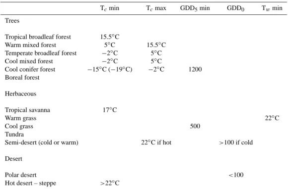
Table 1. Constraints used to compute the biome distribution from the PFTs simulated by the VECODE vegetation model. Tcis the coldest

month temperature, Twthe warmest month temperature, GDD5and GDD0are the standard 0 and 5 degrees Growing Degree-Days (see for

example Prentice et al., 1992). “Tcmin” means a constraint on the minimum allowed for coldest month temperature, “Tcmax” means a

constraint on the maximum allowed for the coldest month temperature.

Tcmin Tcmax GDD₅min GDD₀ Twmin

Trees

Tropical broadleaf forest 15.5◦C

Warm mixed forest 5◦C 15.5◦C Temperate broadleaf forest −2◦C 5◦C Cool mixed forest −2◦C 5◦C

Cool conifer forest −15◦C (−19◦C) −2◦C 1200 Boreal forest Herbaceous Tropical savanna 17◦C Warm grass 22◦C Cool grass 500 Tundra

Semi-desert (cold or warm) 22◦C if hot >_{100 if cold}

Desert

Polar desert <₁₀₀

Hot desert – steppe >₂₂◦_C

In addition to the PMIP boundary conditions, we took the dust forcing due to the ice-age atmospheric dust load-ing (Claquin et al., 2003) into account in the incomload-ing solar radiation at the top of the atmosphere. Also, the lower glacial CO2levels are taken into account in the vegetation part (Har-rison and Prentice, 2003) of the LOVECLIM model. We then applied these forcings to the model’s equilibrium LH CTRL state and integrated it until a new equilibrium was reached, after about 5000 years of integration.

2.3 Biome estimations from VECODE

To better compare the results of VECODE (Brovkin et al., 1997) with proxy data, we have developed a module to com-pute biomes, using both VECODE and ECBilt output. This module is based on the approach of Prentice et al. (1992), with some simplifications. We here considered only the 12 biomes thought to be the most appropriate with respect to the level of the complexity of the VECODE vegetation model and the resolution of the ECBilt atmospheric model. In par-ticular, VECODE only computes two main Plant Functional Types (PFTs): herbaceous and trees. The “tree” PFT is split in terms of needleleaved and broadleaved trees. It also com-putes a desert fraction. The sum of the three fractions (trees, herbaceous and desert) equals one. In cells with a prescribed ice-sheet, we assign all PFTs’ fractions to zero and the desert

fraction to 1. The environmental limits used to convert the PFT distribution computed by VECODE are given in Table 1. For each cell, we first compute the dominating PFT in the cell and then apply the environmental constraints in order to as-sign a biome. In contrast with Prentice et al. (1992), we did not retain any biomes based on the dominance of shrubs as they are not a PFT in VECODE.

Additionally, we have added a tree growing limitation with respect to CO2in order to take into account the effect of higher herbaceous competitiveness under lowered atmo-spheric CO2conditions (Harrison and Prentice, 2003), as has been the case during the LGM.

3 Overview of the simulated LGM climate

3.1 Surface Air Temperature (SAT) changes

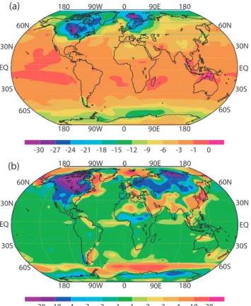
The simulated LGM climate we obtain presents a reduction of −4.4◦C in global mean surface temperature. This re-sult compares well with the PMIP2 models’ mean changes of −4.45◦C (Kageyama et al., 2006, for 6 models) in air temperature. Figure 1 presents the change in global surface temperature between LGM and LH CTRL, together with the changes in seasonal amplitude simulated under LGM condi-tions with respect to LH CTRL.

-20 -10 -4 -3 -2 -1 1 2 3 4 10 20 (a) (b) -30 -27 -24 -21 -18 -15 -12 -9 -6 -3 -1 0 180 90W 0 90E 180 60N 30N EQ 30S 60S 180 0 90W 180 60S 30S EQ 30N 60N 180 90W 0 90E 180 60N 30N EQ 30S 60S 180 0 90W 180 60S 30S EQ 30N 60N 90E 90E

Fig. 1. Changes in simulated SAT at the LGM with respect to the

LH CTRL (in◦C). Panel (a) shows the annual SAT anomaly LH CTRL) over the globe. Panel (b) show the anomaly (LGM-LH CTRL) in seasonal range, defined as being the warmest month minus the coldest month surface air temperature for each of the two climates. All panels show averages over the last 200 years of the simulations.

Changes in SAT (Fig. 1a) show much colder temperatures on the prescribed permanent ice-sheet (up to −30◦C in the centre of Laurentide and Fennoscandian ice-sheets, and up to −6◦_{C at the border) due to the changes of altitude and} albedo. Differences of −6 to −15◦_{C are simulated over the} additional sea-ice covered regions as a response to seasonal or perennial isolation from the atmosphere and albedo effect. Nearby land points also exhibit comparable changes due to the albedo effect of increased snow cover. A cooling of 1 to 2◦C is simulated in most of the tropical and equatorial regions with the exception of no changes over the north of Australia (Sea of Arafora).

We define the seasonal range as being the warmest– coldest month anomaly in surface air temperature. LGM to LH CTRL differences in seasonal range are shown in Fig. 1b. The seasonal range at the LGM is increased globally by 9.7◦C with respect to the LH CTRL simulation. This num-ber however hides large regional differences. We can distin-guish three different zones. a) LGM ice-sheet regions like North America and Scandinavia where the seasonal range is

much less than in the LH CTRL simulation (−4 to −20◦_C). This is due to the fact that these regions have a high sea-sonal range in the present-day, but the seasea-sonal differences are dampened by the all-year cold climate of the LGM, due to the presence of the ice-sheets (this also holds for the Patag-onian ice-cap). This is also true for nearby regions like Siberia, where the seasonal range is reduced due to longer snow cover and cooler summers. b) Regions where there are already ice-sheets in the present-day (Greenland, Antarc-tica) and over oceans between 40◦N and 40◦S. These re-gions undergo small SAT seasonality changes with respect to the LH CTRL (−1 to 1◦C), as they are much unchanged by the LGM climate (mainly cooled down by a few degrees). c) Continental regions in general (and extended deserts in particular) and oceans near ice-sheets and regions with ex-tended sea-ice cover which have a much higher seasonality in the LGM than in the present-day. All these regions are much colder at the LGM during winter time (extension of sea-ice enhanced the effect, neighboring ice-sheet implying snow cover, colder inland and bright desert regions – all an albedo effect, mainly).

3.2 Changes in the hydrological cycle

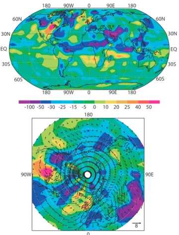
In the global mean, there is a decrease of the total amount of precipitation by 13 mm yr−1, consistent with a decrease in the evaporation due to the global cooling (see Fig. 2a). Some regions undergo a drastic reduction in the rate of an-nual mean precipitation, such as the southern border of the Sahara, the middle- and far- East, some parts of central Asia (in particular the Tibetan Plateau) and central Greenland – a feature consistent with snow accumulation data (Cuffey and Clow, 1997; Alley, 2000) – and Western Canada. There is also some consequent diminution of precipitation in south-ern Europe – consistent with both other model results and proxy data (Tarasov et al., 1999; Peyron et al., 2005; Jost et al., 2005) –, some parts of Siberia, Svalbard, Japan and southern America (Argentina and southern Chile). The de-crease of precipitation observed in South America is consis-tent with the fact that this region was a source of dust in the LGM (Grousset et al., 1992; Basile et al., 1997).

As can be inferred from Fig. 2b, the changes in precipi-tation occurring in the Northern Hemisphere are mainly due to the displacement of the winds tracks, as a consequence of the presence of ice-sheets. Interestingly, the simulated changes show a maximum increase of precipitation over the southern border of the Laurentide ice-sheet (a feature also re-ported by Kageyama and Valdes, 2000, and Vettoretti et al., 2000) and on the western flank of the Fennoscandian ice-sheet. The increase in precipitation over these areas is cru-cial for maintaining ice-sheets at the LGM, both for the southern part of the Laurentide ice-sheets, which presents a lobe advance in this region (Peltier, 2004), and for the Fennoscandian ice-sheet. It is an important pre-requisite to be able to simulate the advance and volume of the last glacial

ice-sheets, especially the Fennoscandian one (Forsstr¨om and Greve, 2004; Charbit et al., 2006).

The changes in the precipitation pattern in the LGM there-fore seem to be quite comparable with other LGM studies (Vettoretti et al., 2000) as well as favourable to maintain the extensive (prescribed here) ice-sheet of the LGM period.

3.3 Changes in simulated vegetation cover

Globally the simulated changes in vegetation cover are re-sponses to the cooler and dryer conditions which prevail in the simulated LGM climate described here. For the three Plant Functional Types (PFTs) simulated, VECODE simu-lates the following evolutions in the LGM with respect to LH CTRL (not shown).

The desert fraction is expanded in central Asia, the Sa-hara and southeast America, reflecting the drier conditions prevailing there. Some polar desert appears in northeast-ern Siberia (which denotes extreme cold and dry conditions, compatible with the absence of an ice-sheet in this area dur-ing the LGM, see Svendsen et al., 2004).

Tree fractions are reduced overall, as low as zero in cer-tain regions. For example, the cooling of the climate and the lowering of the atmospheric CO2level causes disappear-ance of the LH CTRL forests of central Russia and Siberia in favour of herbaceous areas. The model furthermore simu-lates the shrinking of the tropical broadleaf forests (Amazo-nia and tropical Africa) in response to drier conditions (see Fig. 2a). In the case of northern America, we can make a di-rect comparison between simulated PFTs and proxy-based reconstructions for the tree cover in the LGM (Williams, 2002). VECODE correctly simulates a mixture of needle-leaved and broadneedle-leaved trees on the east coast of America, with a high tree cover until the southern boundary of the Laurentide ice-sheet. The central part of the United States is correctly covered predominantly by grass with few trees (0–15%). However, our simulation shows dense tree cover in the western United States for the LGM, a feature which is not seen in proxy data (Williams, 2002). This feature is also present in the LH CTRL simulation which shows a too large tree cover in this region for the Late Holocene. This is due to the too humid state simulated in this area for both climates.

Grass fractions are increased in regions where the tree area shrinks, and in particular in central Asia, southern Europe, western Africa and eastern Brazil.

All these changes are broadly consistent with the changes found in pollen distributions for the LGM (Prentice et al., 2000, for example). However, as it is common to describe the reconstructions of vegetation in terms of biomes, we consid-ered it useful to develop an approach that computes biomes from the available PFTs distribution and climatic variables in a simple manner (as presented in Sect. 2.3). The results obtained in this development are described in Sect. 4.1, and enable a detailed data-model comparison for our simulated LGM climate. -100 -50 -30 -25 -15 -5 0 10 20 25 40 50 8 180 90W 0 90E 180 60N 30N EQ 30S 60S 180 0 90W 180 60S 30S EQ 30N 60N 90W 0 180 90E 90E

Fig. 2. Changes in simulated precipitation at the LGM with respect

to the LH CTRL (in mm yr−1). Panel (a) shows the precipitation anomaly (LGM-LH) over the globe. Panel (b) shows the precipita-tion anomaly (LGM-LH) for the Northern Hemisphere, with LGM to LH CTRL changes in the wind field (at 850 hPa) superimposed as vectors. All panels show averages over the 200 last years of the simulations.

3.4 Changes in the deep ocean circulation

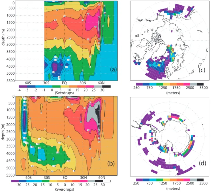
The location of deep water formation in the Northern Hemi-sphere is shifted from the Labrador and Nordic seas for LH CTRL to the south of Iceland and Greenland in our LGM simulation, with some convection remaining in the Nordic seas (Fig. 3c). These changes are accompanied by a reduc-tion of the maximum depth of direct ventilareduc-tion by about 600 m. The maximum convection depth is still reached in the Nordic seas (1800 m), marginally deeper than south of Iceland (1400 m). However, the convection site south of Ice-land is more permanent, whereas the activity of the Nordic Seas site depends on the year considered.

In the Southern Hemisphere there are few changes in the depth reached by convection, but an important shift in the lo-cation of deep water production is noted (Fig. 3d). Whereas in LH CTRL sinking waters are formed partly along the coast of Antarctica (plus the Weddell and Ross seas) and partly further away from the continent, this latter source

(meters) depth฀(m) depth฀(m) (meters) -4 -3 -2 -1 0 5 10 15 20 25 30 0 500 1000 1500 2000 2500 3000 3500 4000 4500 5000 5500 _{60S 30S EQ 30N 60N} 250 750 1250 1750 2500 3500 250 750 1250 1750 2500 3500 60S 30S EQ 30N 60N 0 500 1000 1500 2000 2500 3000 3500 4000 4500 5000 5500 -30 -25 -20 -15 -10 -5 10 15 20 25 30 (Sverdrups) (Sverdrups)0

(a)

(b)

(c)

(d)

Fig. 3. LGM Meridional overturning streamfunction for the Atlantic (panel a) and the world (panel b) oceans. Contours are in Sverdrup,

positive (respectively negative) values denote clockwise (resp. counterclockwise) flow. LGM maximum convective depth around Antarctica (panel d) and in the north Atlantic and Nordic Seas (panel c); depth is labeled in metres. Panels (a) and (b) show averages over the 200 last years of the simulation, panels (c) and (d) maximum over the same time interval. We show the maximum convective depth, thought to be more indicative of the real depth attained by the deep water masses.

disappears in the LGM simulation and the former is rein-forced. There is open ocean convection along the coast of Antarctica in all sectors of the Southern Ocean, the strongest and deepest being in the Atlantic sector. As a result of this shift in the location of convection, there is a strong enhance-ment of AABW production that is doubled in the LGM sim-ulation with respect to LH CTRL. This evolution is related to a decrease of sea-ice production on the continental shelf in the LGM compared to LH CTRL, the large sea-ice extent obtained promoting sea-ice formation further away from the continent.

The total rate of North Atlantic Deep Water (NADW) for-mation is stronger in the LGM simulation than in LH CTRL. The associated meridional overturning streamfunction is shown in Fig. 3 (see Appendix A for LH CTRL results). The simulated oceanic water export at 20◦S is about 16.4 Sv with respect to a 13.8 Sv LH CTRL value (enhanced by 2.6 Sv), as is shown in Fig. 3a. The input of AABW in the Atlantic at 20◦S is 2.6 Sv in the LGM compared to 7 Sv in LH CTRL, thus experiencing a decrease of 4.4 Sv. This is in contra-diction with the prevailing view of the LGM Atlantic ocean circulation, which is believed to be less active, shallower,

1 2 3 4 5 6 7 8 9 10 11 12

Tropical forest Warm mixed forest Temperate broadleaf forest

Cool mixed forest Cool conifer forest Boreal forest Tropical savanna Warm grass Cool grass Tundra Semi-desert (cold/warm) Polar desert Hot desert - Steppe

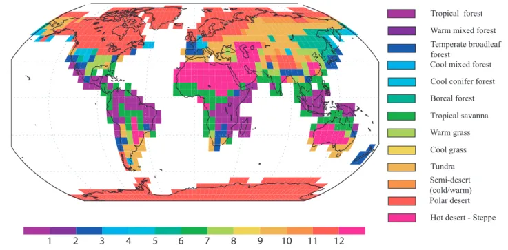
Fig. 4. Estimated biomes in the LGM simulation. See Sect. 2.3 for the method of estimation.

and with an increased AABW import in the Atlantic basin (Ganopolski et al., 1998; Rahmstorf, 2002; Shin et al., 2003). There is however no agreement on the strength of the glacial thermohaline circulation in coupled model simulations of the LGM (Hewitt et al., 2003; Mix, 2003; Shin et al., 2003; Timmermann and Goosse, 2004; Kim, 2004), some obtain-ing stronger overturnobtain-ing and some weaker. In fact, a re-cent comparison of the LGM ocean circulations in different PMIP simulations (Weber et al., 2007) showed that half of the models produce an increase in overturning rate under glacial boundary conditions. In particular there is much debate on the relative strength of the Glacial Antarctic Bottom Wa-ter (GAABW) and Glacial North Atlantic Deep/InWa-termediate Water (GNADW/GNAIW) in the LGM (Paul and Sch¨afer-Neth, 2003). The relative proportion of these water masses is being controlled by the relative density of the two; to ob-tain a stronger inflow of deep Antarctic water, this water mass should be much denser than that of the deep north At-lantic. In our simulation, the GNADW is slightly denser on average than the GAABW, which then prevents considerable AABW presence in the Atlantic basin. There are however some multi-centennial variations in the deep convection, with periods of reduced GNADW formation in the GIN seas, en-abling the entrance of more GAABW – more than a doubling during one to two hundred years. The simulated ocean state is thus variable, so that the average state may not be the most appropriate view of it (Hewitt et al., 2006). In Sect. 4.5 we will critically discuss the state obtained here with respect to available data.

4 Model-data comparison

4.1 Simulated vegetation

In this sub-section, we discuss the simulated vegetation in our LGM climate in terms of biomes with respect to available reconstructions (see Table 1 for the bioclimatic ranges used in classification). Hereafter, we discuss each main regions separately; the biomes discussed are presented in Fig. 4.

1. Siberia. In the model, we simulate the disappearance of much of the present-day boreal forest type which is replaced by a mixture of tundra and cool grass types. The non-glaciated area of the northwestern Alaska and Beringian regions are defined as the tundra biome type. These results are more or less in line with available proxy data, in particular with the Bigelow et al. (2003) compilation which depicts different types of tundra over Bering, a small part of northwestern Canada and north-ern Siberia, except for two sites in Siberia with Temper-ate Grassland biome (Bigelow et al., 2003; Kaplan et al., 2003) which replaces the Siberian cool-mixed/boreal forests existing in the present-day.

2. We simulate in southwestern Europe a mixture of tem-perate trees and cool grass biome types. This reflects the too warm/moist conditions prevailing south of the Fennoscandian ice-sheet in our simulation; this feature is not consistent with available data for this region. Cool grass is attributed as the dominant biome in southeast Europe. This second part is much in line with the

compilation of Ray and Adams (2001) which depicts southern Europe as being dominated by steppe-like con-ditions with some trees in the more moist areas, and also with the compilation of Prentice et al. (2000).

3. In northern Africa, there is a general drying, promot-ing the southward extension of the desert regions – Sa-hara type – by 5 to (locally) 11◦, at the expense of the tropical Savanna simulated in the LH CTRL simulation. This result is fairly consistent with the southward exten-sion of the Sahara desert boundary by 5◦of latitude, as depicted by Prentice et al. (2000) and Ray and Adams (2001).

4. The regions of tropical forest in central Africa, although already too small in extension in the LH CTRL simula-tions, are nevertheless smaller in the LGM simulation, with the disappearance of this particular biome along the Atlantic seaboard. Conversely, the tropical forest cover, too extensive already at present-day on the In-dian side, is preserved in our LGM simulation. The shrinking – without disappearance – of the tropical for-est areas in central-wfor-est Africa is in line with current reconstructions (Dupont et al., 2000; Ray and Adams, 2001; Leal, 2004), although our simulation of extensive tropical forests on the Indian ocean side is unrealistic. This discrepancy between data and model is also found in South America, and is due to an incorrect represen-tation of the zones of high precipirepresen-tation in the ECBilt model, promoted on the eastern side of the continents instead of more central regions.

5. Central Asia is a place of great expansion of desert and semi-desert biomes in our LGM simulation with respect to the LH CTRL, with, in particular, the appearance of a great desert in central China, surrounded by a cool grass biome replacing most of the simulated LH CTRL warm grass/cool forest. Some regions of tundra and cold semi-desert slightly expand around the Tibetan plateau. Not many changes are seen in the tropical belt (India, south-east Asia and Indonesia) with respect to the LH CTRL simulation, albeit from slight drying conditions inland in southeast Asia. Japan sees the replacement of a mix-ture of warm/temperate forest in the LH CTRL simu-lation with a complete cover of temperate forest in our simulated LGM. All these features are broadly consis-tent with the current compilations. Some discrepancies are however notable; in general the model simulates a too wide extension of forests in northeast China and southeast Asia, whereas pollen estimations yield more steppish conditions in those areas. Ray and Adams (2001) mention the expansion of deserts in central Asia and the shrinking of tree cover in China. The LGM veg-etation of Japan is seen as a mixture of cool mixed forest to temperate forest in data (Prentice et al., 2000), not in-consistent with our simulated dominance of temperate

forest, although the data suggests colder conditions in the northern part.

6. As already discussed, south of the Laurentide ice-sheet we simulate the cover of tree and grass relatively well according to proxy data available for these PFTs (Williams, 2002). In terms of inferred biomes, central U.S.A. is covered by the “warm grass” biome in our simulation, whereas reconstructions point to “tundra” (Prentice et al., 2000) or “temperate grassland” (Ray and Adams, 2001). The absence of trees in our re-sult is thus consistent with these reconstructions. On the eastern Atlantic coast we simulate a bioclimatic gradient from “tropical savanna” (in Florida) to “tun-dra”/“temperate forest” (at the ice-sheet border). In data these regions are depicted as ”open conifer woodland” in Florida to “taiga” of “cool mixed forest” in the north (Prentice et al., 2000; Ray and Adams, 2001). There-fore, the model exhibits some exaggeratedly warm con-ditions in southeastern USA with respect to data, but is not too far off at the ice-sheet border. Towards the Pa-cific coast, we obtain a mixture of “temperate forest” to “cool conifer forest” with some tundra, compared to “tundra” and “cool conifer” in data (Prentice et al., 2000). This area seems therefore quite consistent with proxy data. Southward we have a fairly extensive cover of “tropical forest” in Central America, outlining the too humid conditions we simulate there compared to data (Ray and Adams, 2001).

7. In South America, our estimated biomes show two main patterns: a slight northwards migration of the Amazo-nian forest by 5 to (locally) 11◦_{of latitude and a general} drying of the Argentinian and Uruguayan regions (semi-desert and cool grass biomes). These results for the Amazonian forest are in line with proxy data, although the state of the Amazonian forest at the LGM is still quite controversial (Colinvaux and de Oliveira, 2000; Ray and Adams, 2001; Leal, 2004, for example). The drying of the southeastern part of South America (and especially of the shelves exposed during the LGM) is seen in data, and recorded as dust deposits in the Antarc-tic ice-cores. We also find some areas of desert and semi-desert in south America (Ray and Adams, 2001). 8. Finally our simulation of vegetation in Australia shows

an important increase of the desert and semi-desert biomes in our LGM simulations at the expense of the forest cover (LH CTRL), which is limited to the coast-line. These results are in good agreement with cur-rent reconstructions which show extreme desert in the centre of Australia with overall less forest cover (Ray and Adams, 2001; Prentice et al., 2000). In north-ern Australia, we simulate drier grass-dominated condi-tions in line with available data. The simulated savanna does not have a significant fraction of trees, therefore

representing the dry and open conditions prevailing in this area at the LGM.

4.2 Land temperatures: permafrost in Europe

A good indicator of the mean cooling of the climate is the limit of the permafrost. In this sub-section, we therefore try to compare the simulated LGM climate with data for the per-mafrost limits in Europe, following the types and limits of Renssen and Vandenberghe (2003), namely: 1) discontin-uous permafrost exits if annual mean temperature is below

−4◦C and 2) continuous permafrost exists if both mean an-nual temperature is below −8◦C and the coldest month tem-perature is below −20◦C.

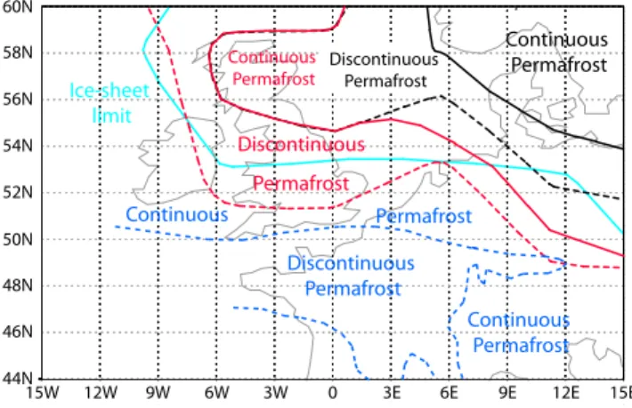
Figure 5 shows the limits of the continuous and discontin-uous permafrost as simulated for the LGM with the limits es-timated from proxy data. It is striking that the simulated area of permafrost is much too small with respect to proxy data, with continuous permafrost simulated only for Scandinavia and the Baltic States whereas it should extend up to Bel-gium, the south of Germany and all off the United Kingdom and Ireland (Renssen and Vandenberghe, 2003). This under-estimation indicates that we overestimate temperatures over western Europe, which is related to the anomalously warm conditions over the nearby Atlantic Ocean (see Sect. 4.3). Moreover, we do not simulate continuous permafrost over the British Isles, even if there is a prescribed ice-sheet over their northern reaches. This is probably due, in part, to the resolu-tion of the model: the ice-sheet is prescribed only over a part of the grid-cells in this area, the rest being ocean. Therefore, the continentality is certainly underestimated when close to the oceanic regions (this is also true for other regions like France, Belgium and the Netherlands).

To evaluate how much of the mismatch between model and data is attributable to this continentality effect and to dis-entangle it from a more global climatic mismatch, we have conducted a sensitivity experiment with a modified land-sea mask for the ECBilt (atmospheric) model. We arbitrarily as-signed all grid-cells containing some land a new value of 95% land, to artificially increase the continentality of the more inland points. This set-up leads to some inconsistencies between the atmospheric and oceanic models (ECBilt and CLIO); we therefore only integrate it for 100 years to gain an idea of the atmospheric effect without allowing the ocean time to be modified. Results are also presented in Fig. 5, in terms of permafrost. The limit of continuous permafrost is shifted southwards to the north of The Netherlands and across southern Germany and Ireland. It is not in perfect agreement with proxy data (especially with the absence of discontinuous permafrost in France) but is nevertheless im-proved.

The southernmost winter sea-ice limit is also modified in this “continentality” experiment, from the south of Nor-way (north of Scotland) to the south of Scotland, along the coast of the United Kingdom. This therefore shows that

Discontinuous฀ Permafrost Continuous฀ Permafrost Permafrost Continuous฀

Permafrost Discontinuous฀Permafrost Discontinuous฀ Permafrost Continuous฀ Permafrost Continuous฀ Permafrost Continuous Permafrost Ice-sheet฀ limit Discontinuous 60N 58N 56N 54N 52N 50N 48N 46N 44N 15W 12W 9W 6W 3W 0 3E 6E 9E 12E 15E

Fig. 5. Permafrost in western Europe: data and model. Lim-its of permafrost are outlined as follow: continuous black line (respectively dashed black line) is the continuous (respectively non-continuous) permafrost limit for the simulated LGM, contin-uous red line (resp. dashed red line) is the contincontin-uous (resp. non-continuous) permafrost limit for the “continentality” sensitivity ex-periment (see text) and continuous dark blue line (resp. dashed dark blue line) is the continuous (respectively discontinuous) permafrost limit inferred from data (Renssen and Vandenberghe, 2003). The continuous light blue line is the limit of the imposed ice-sheet in the atmospheric part of the model.

the relationship between permafrost and sea-ice proposed by Renssen and Vandenberghe (2003) in an atmospheric-only model is also found to some extent in a coupled ocean-atmosphere model.

The climate of southern Europe still remains too warm with this drastic set-up, implying that it depends on the simulated sea surface temperatures (which are not much modified in 100 years). We therefore suggest that simu-lated sea-surface temperatures are too warm in the eastern north Atlantic in our simulated LGM, as discussed hereafter. The method to improve these temperatures is non-trivial, but could encompass the modification of the Mediterranean treatment in the model.

4.3 Surface ocean

The goal of this part is to provide a first simple comparison between MARGO data of the glacial surface ocean and our simulated LGM state.

4.3.1 Sea-ice distribution

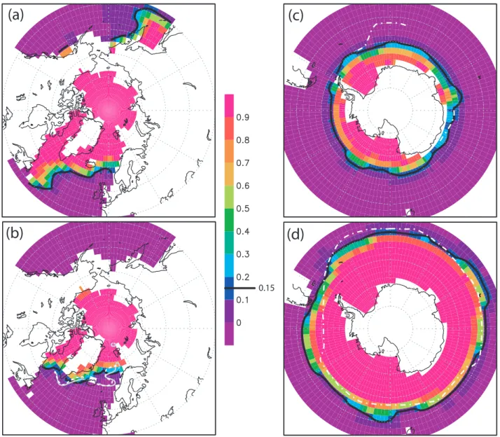
For the Northern Hemisphere, there is a considerable in-crease of the sea-ice area compared to LH CTRL, but in a spatially non-homogeneous fashion (see Fig. 6, panels a and b). The summer extent in our simulated LGM is comparable to our present-day winter, with sea-ice covering the Labrador Sea, the Arctic (quasi-continuously) and a small part of the Nordic Seas, almost to the north of Norway. There is also

0.15

(a)

(b)

(c)

(d)

Fig. 6. Sea-ice concentration simulated for the LGM with comparison to MARGO data. Panels (a) and (c) are for the austral summer, (b)

and (d) for the boreal summer. Sea-ice concentrations are plotted according to the common colour bar in the centre, with a black contour at 15%, to enable easy sea-ice limit comparison with data of Gersonde et al. (2005); the averaging is performed over the last 200 years of the simulation. On panel (b) (Northern Hemisphere, boreal summer) the dashed white line and the continuous grey line indicate seasonal ice-free conditions from Kucera et al. (2005b). On panels (c) and (d) the dashed-dotted white line shows the summer (c) and winter (d) 15% sea-ice concentration as from Gersonde et al. (2005).

some sea-ice maintained along the coast of Greenland. If compared with estimations for the limit of seasonal ice-free conditions provided by Kucera et al. (2005b), our simulated sea-ice cover agrees fairly well, except over the eastern At-lantic. In particular, we faithfully reproduce the ice-free con-ditions prevailing over most of the Nordic Seas and the more extensive southwards extent on the western Atlantic, espe-cially along the coast of Greenland. The simulated boreal winter sea-ice extent shows an important increase of espe-cially along the coast of Newfoundland extending far into the western Atlantic. Conversely, on the eastern side, the

winter extension is much more limited, to the south of Ice-land and Norway. This shows the effect of the still active north Atlantic drift which, by warming the surface waters, enables ice-free conditions in an important part of the eastern Atlantic. The sea-ice cover is probably somewhat underesti-mated: given the presence of an ice-sheet covering Scotland and the north of Ireland, it is probable that sea-ice also ex-isted there during winter, at least along the coast. Part of the answer probably lies in the coarse, T21, resolution of the at-mospheric model. At this resolution (5.6◦ latitude by 5.6◦ longitude) the Brittish ice-sheet has a very low altitude and

the land-sea distribution is poorly represented along conti-nental margins.

For the Southern Hemisphere, there is generally a rea-sonable agreement between the sea-ice concentrations in our simulated LGM climate and proxy data (Crosta and Pichon, 1998a,b; Gersonde and Zielinski, 2000; Gersonde et al., 2005), as can be seen in Fig. 6, panel (d). Some model-data discrepancies exist in certain areas. We overestimate slightly the sea-ice cover occurring at the transition between the Pacific and the Atlantic sector in the Southern Ocean, par-ticularly in the southwest of the Magellan archipelago. We also slightly underestimate the sea-ice cover in the southern Atlantic during winter. The simulated sea-ice concentration for the austral summer is consistent with data in the Indian sector, but compares less favorably with data for the Atlantic sector. The model captures fairly well the asymmetry be-tween the Indian sector, where the summer sea-ice extent is comparable to that of today’s, and the Atlantic sector, where it is more extensive. However, it fails to reproduce the large extent of sea-ice between −5◦E and 5◦W. There are two options to account for this discrepancy: either the limit de-rived from the diatoms is for the particularly cold summers or there is a spreading of sea-ice which is not represented in the model. The former option, though the sea-ice extent is de-noted as “sporadic” (Gersonde et al., 2005), seems however not to be the most probable: Gersonde et al. (2003) rather point to a local expansion due to specific Weddell Sea dy-namics, which, we believe, are not represented in the CLIO model.

4.3.2 Sea surface temperatures

Here we provide an outline of the data-model comparison between our LOVECLIM results and MARGO data for the annual mean SST and LGM to LH difference, to better posi-tion the state of the simulated LGM climate. The MARGO project released an extensive coverage of Sea Surface Tem-perature (SST) estimates for the LGM for a wide range of proxies. It is beyond the scope of the present study to com-pare in detail the results obtained here with the MARGO database, especially taking into account that not only annual average SSTs are provided, but also in most cases those for summer and winter (see Kucera et al., 2005a, and compan-ion papers). We will follow an approach comparing differ-ent regions: Indian Ocean and Australian margins, Pacific, Southern and Atlantic Ocean.

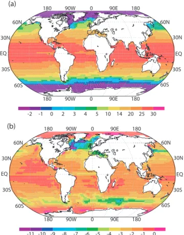
For the Indian Ocean and the Australian margins, the model indicates differences of −1 to −2◦_{C relatively} homo-geneously, in good agreement with proxy data (Barrows and Juggins, 2005). Indeed, in terms of mean annual SST anoma-lies between LGM and present-day, proxy data broadly show a general moderate cooling of the equatorial regions of 0 to 3◦C. Some data points for the equatorial Indian ocean even indicate no changes or a small warming. In the tropical re-gions, the Gulf of Bengal and the Arabian Sea show a very

(a) (b) 180 90W 0 90E 180 60N 30N EQ 30S 60S 180 90E 0 90W 180 60S 30S EQ 30N 60N -2 -1 0 2 3 4 5 10 14 20 25 30 180 90W 0 90E 180 60N 30N EQ 30S 60S 180 90E 0 90W 180 60S 30S EQ 30N 60N -11 -10 -9 -8 -7 -6 -5 -4 -3 -2 -1 0

Fig. 7. (a) Sea Surface Temperatures at the LGM (◦C) (b) LGM-LH CTRL Sea Surface Temperature differences (◦C). Both panels are averages over the last 200 years of the simulations.

small cooling, with no change or less than 1◦_{C cooling. This} feature is not seen in our simulation, which yields a cooling by 1 to 2◦C, and even some greater cooling along the coast of India. The reason for this mismatch is not clear, and would need to be further investigated. Changes are of greater mag-nitude in proxy data to the south, with cooling of 3 to 5◦C at 30–35◦S south of Madagascar.

This is also more or less the case in the model, which sim-ulates cooling of 2 to 4◦C in the same area. Around 40◦S, eastward from the Kerguelens, data show a more pronounced cooling, between 3 and 5◦C; this feature is also well marked in the simulated LGM where cooling reaches 3 to 5◦C. In this region, we find the greatest simulated cooling in the Southern Hemisphere ocean, with about 8◦_{C. These huge changes are} linked to the northwards migration of the Polar Front and of the Antarctic sea-ice margin, which promote the northward expansion of colder waters. Finally, the biggest changes oc-cur in the Pacific Ocean, east of Australia, where there is a cooling of 3 to 5◦C at 30◦S, and up to 7–8◦C over the Camp-bell Plateau, southeast of New Zeeland. These changes are qualitatively well represented in the model which simulates a −3 to −4◦C change off the eastern coast of Australia, and 4 to 5◦C cooling at the Campbell Plateau. However, we do

not reach the extreme cold shown by proxy data in the latter region.

For the nearby Pacific, data are more sparse, but still show some patterns which we can compare to our simula-tion (Kucera et al., 2005b). The equatorial Pacific, as re-constructed, shows little changes (assigned as −1 to 1◦C), but with slightly cooler temperatures on the South American side (−1 to −3◦C). This is also the case in our simulation, which presents an homogeneous cooling of 0 to 1◦C in the equatorial region, with the exception of slightly cooler tem-peratures along the south American coast (−1 to −2◦C). We simulate 1 to 2◦C cooling in the Pacific warm pool, quite in line with independent proxy data estimates (Chen et al., 2005). At 30◦N, the reconstructions show no clear signal (ranging from +1 to −3◦C) to compare to our simulated 2 to 4◦_{C cooling. Northeast of Japan, around 50}◦_{N, data show an} LGM to LH CTRL cooling of about 1 to 3◦_{C or even more;} our simulation compares relatively well with a −2 to −4◦_C changes in this region. Finally, our simulation does not re-produce the cooling of more than 3◦C seen in proxy data for the American coast at 40◦N. In particular, proxy data show an annual mean temperature of about 8◦C at this loca-tion whereas the model simulates an annual temperature of about 12 to 14◦C, a temperature barely reached in the proxy data 10◦ westward. Two possibilities could be further in-vestigated: the first would be the role of coastal effects, the second of the extension of sea-ice in the northeastern Pacific (non-existent in our simulations, see Fig. 6) both in relation-ship with the evolution of the California current.

Around Antarctica, our model simulates an important cooling, with an annular pattern around the continent, quite in line with proxy data of Gersonde et al. (2005). This seems a logical counterpart of the good ability of the model to sim-ulate the sea-ice in this region.

For the Atlantic, our simulations produce general changes quite consistent with proxy data (Pflaumann et al., 2003; Kucera et al., 2005b) for equatorial regions (−2 to −4◦C in both data and model) and the 20◦N band (0 to −1◦C in data vs. −1 to −2◦C in the model. The agreement holds for the mid-latitude Atlantic further to the north where the model simulates a cooling from 2◦C at 30◦N to 4◦C around 40◦N and proxy data suggest a cooling of −1 to −4◦C. There is however an important mismatch in the more northern re-gions: the model simulates the maximum cooling along the American coast whereas this is found off the coast of Ireland according to proxy data. This mismatch may be due to model poor representation of the northern Atlantic gyre circulation in our model, or the treatment of the Mediterranean Sea, as discussed below. Model–data discrepancies in this area are a common feature already recognised in several coupled mod-els (Kageyama et al., 2006).

In the Mediterranean sea, although the resolution of the model is too low to simulate the dynamics occurring here in detail, we obtain a broad agreement with proxy data (Hayes et al., 2005). We simulate anomalies ranging from −5 to

−6◦_{C in the western part (−6}◦_{C in data) to −3 to −4}◦_{C in} the eastern part (−2 to −3◦_{C in data).}

To summarise, generally our simulated SSTs are consis-tent with data in most areas. We have discussed some mis-matches in specific regions. The causes of these mismis-matches may be diverse, but several seem to be linked to the displace-ment of oceanic fronts or local currents, features difficult to simulate with accuracy. The precise cause of these mis-matches should be further investigated.

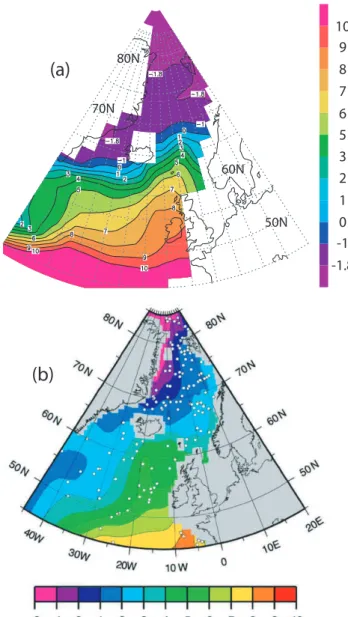
4.4 Subsurface northern Atlantic and Nordic seas

Given the importance of the north Atlantic Ocean and Arc-tic Seas in producing part of the deep waters of the world ocean, we perform here a more detailed comparison between the modeled and proxy-based subsurface temperatures (Me-land et al., 2005), as shown in Fig. 8. Our results (panel a) are given on the same projection and scale for ease of com-parison with temperatures estimates from δ18O (see panel b, reproduced from Meland et al., 2005).

Data presented show a fairly strong east-west gradient, from quite high temperatures (8 to 9◦C) off the coast of France to much lower temperatures (1 to 3◦C) south of Greenland at the same latitude. This gradient is present all the way to Svalbard, but weakens to a 3◦C difference be-tween east and west along Iceland, similar at the south of the Svalbard. In our simulated LGM, such a gradient also exists (linked to the presence of the (glacial) north Atlantic Drift) but it is of correct magnitude only around the north of Ire-land (6◦C difference from 9◦C on the east coast to 3◦C to the west). South of about 50◦N, the model shows fairly homoge-neous relatively high annual temperature (more than 10◦C). These waters of quite high temperatures entering the eastern Atlantic originate from a mixture of lower latitude Atlantic waters and Mediterranean Sea water of higher temperatures. Due to the relatively coarse resolution of the model, the strait of Gibraltar is much wider than in reality. Therefore, the ex-change seems to be too important at the LGM between the Mediterranean Sea and the Atlantic Ocean. This is likely to be the source of the 2 to 3◦C overestimation off the coast of Ireland.

Northwards, the model results are fairly comparable to data, with only about 1◦C difference, and a very similar east-west pattern, indicating that we capture correctly the entrance of north Atlantic waters in the Nordic Seas. The influence of the north Atlantic waters entering the Nordic seas extends up to the Svalbard as can be inferred from the flow vectors (not shown), as is seen in data. For the Nordic seas, our simulated annual temperatures are more homogeneous than those seen in data, with slightly too cold temperatures at the northern tip of Norway. This seems to be linked to a small regional overestimation of the sea-ice cover in that area (see Fig. 6). This explains that the influence of the North Atlantic waters entering the Nordic Seas is less prominent from the temper-ature field than in data. Otherwise, the annual tempertemper-ature in

the Nordic Seas is fairly well represented, with waters close to the freezing point along the western coast of Greenland, suggesting perennial sea-ice cover.

To summarise, the model-data comparison shows that LOVECLIM simulates reasonable annual mean LGM tem-peratures in the northern Atlantic and Nordic Seas, with a more or less correct east-west gradient. A discrepancy is found in the absolute value south of 55◦N, probably linked to the representation of the Mediterranean outflow in a rela-tively coarse resolution model. This latter question needs to be re-addressed in future studies.

4.5 Deep ocean circulation

In this sub-section, we review the LGM state as simulated by the LOVECLIM model for the oceanic circulation with respect to the available proxy data. Different types of proxies are usually used as constraints with the view of determining the palaeoceanographic state of the LGM.

Our simulated LGM state includes three source locations for deep waters: two in the Northern Hemisphere and one in the Southern Hemisphere. As discussed in Sect. 3.4, we find in the Northern Hemisphere a main site south of Iceland, and a secondary location in the Nordic Seas. In LH CTRL, the main site for NADW formation is in the Nordic Seas. The simulated southward shift of the main northern convection site to a location south of Iceland is consistent with proxy data (Labeyrie et al., 1992; Oppo and Lehman, 1993). Proxy evidence also exists for active deep water formation in the Nordic Seas (Dokken and Jansen, 1999) during the LGM, in line with our findings.

A tracer which is often used to characterise oceanic water masses in the past is the δ13C measured in foraminifera tests (Duplessy et al., 1988, for example), used to distinguish be-tween ventilated and less-ventilated water masses. A feature present in any reconstruction of the glacial δ13C is the very strong vertical gradient at 2500 m dividing the Atlantic be-tween an upper well-ventilated water mass and a lower, much less-ventilated, water mass. The current interpretation of this gradient is the existence of two water masses in the Atlantic: the upper one is attributed to the GNAIW (Glacial North At-lantic Intermediate Water), forming south of Iceland, and the lower one to the GAABW (Glacial Antarctic Bottom Water) assumed to form along the Antarctic coast. Thus, defining the δ13C end-members of the (supposed) main water masses allows to evaluate with some accuracy (Duplessy et al., 1988; Curry and Oppo, 2005) the degree of mixing between north-ern and southnorth-ern water masses. For example, in Curry and Oppo (2005), a ratio of 50% of GAABW to 50% of GNAIW is found in the North Atlantic at 3100 m and 30◦_N).

In our LGM simulation, we have three instead of two deep water masses in the Atlantic. We can identify GNAIW that is formed at the main deep convection site south of Iceland, and a second water mass that is formed in the Nordic Seas. This latter water mass is denser than the modelled GNAIW; thus

10 9 8 7 6 5 3 2 1 0 -1 -1.8

(a)

(b)

Fig. 8. Model-data comparison: north Atlantic and Nordic Seas subsurface temperatures. Panel (a) shows the model annual mean temperature (◦C) between 50 and 150 m depth (averaged over 200 years). Panel (b) is an δ18O-based temperature estimation (◦C) re-produced from Meland et al. (2005) (with permission from Else-vier).

we will refer to it as GNADW (Glacial North Atlantic Deep Water). The third water mass is GAABW, with a source in the Southern Ocean. To compare our simulation with δ13C data (Curry and Oppo, 2005), we therefore need to consider three end-members. Regrettably, we do not simulate explic-itly the δ13C in our model, so we are unable to precisely assess its distribution. However, some interesting features should be pointed out. Regarding density properties, the two water masses identified as GNADW and GAABW have characteristics very close to each other (GNADW is warmer and saltier than GAABW, but their densities are similar). In our simulation, both GNADW and GAABW are formed

in sea-ice covered regions, implying that these deep water masses are not well ventilated. Therefore, we would expect the mixture of the two water masses to have δ13C values de-pleted with respect to GNAIW. The exact values for each of the end-members depend on the δ13C content of the waters from which they are formed. However, it seems plausible that the simulated GNADW and GAABW have a δ13C sig-nature close to each other in the deep north Atlantic. There-fore, if this line of reasoning is followed, the obtained ocean would indeed be partitioned between a deep water mass (be-ing a mix between the GNADW and the GAABW, depend-ing on the location) and an upper ocean one (GNAIW). Evi-dences of δ13C data (Curry and Oppo, 2005), showing a very depleted deep water mass (GAABW) entering the south At-lantic (values around −0.8 per mil at 3000 m depth) evolv-ing to a less depleted deep water mass in the northern At-lantic (values around 0.0 per mil at 3000 m depth) are con-sistent with this hypothesis of mixing betwee n GAABW and GNADW masses.

Conversely, Pa/Th ratios measured in the shells of foraminifera, used as a proxy for advection, are linked di-rectly to changes in oceanic circulation. The Pa/Th is a La-grangian tracer and thus integrates changes in transport of water from the source (sinking regions) to the site where it is measured. Therefore, its recorded variation over time at the site may depend on the global circulation (on average, less water advected in the whole north Atlantic and over the site) or a more local change at the site, being more slowly ven-tilated whereas some regions are more venven-tilated. From the three different studies addressing changes in oceanic circu-lation with the Pa/Th, one study (Yu et al., 1996) was aimed at a basin-scale reconstruction of the LGM oceanic circula-tion. They showed that the data obtained were consistent with a strength of the glacial Atlantic meridional overturning similar to that of the present-day. In a later reassessment of the same data with the aid of a model, Marchal et al. (2000) showed that available Pa/Th data is also consistent with a reduction of the strength of the circulation by up to 30%. Fi-nally two recent studies addressed the temporal variation of the thermohaline circulation in the western (McManus et al., 2004) and eastern (Gherardi et al., 2005) Atlantic basins over the last deglaciation. The first one showed that at a depth of 4.5 km in the west Atlantic, the vertically integrated oceanic transport was reduced by 30% at the LGM with respect to present-day. The second one deduced that the vertically in-tegrated oceanic transport in the eastern Atlantic at a depth of 3.1 km was enhanced at the same time. This indicates that: a) the thermohaline circulation was stronger in the first 3 km of the ocean, a feature compatible with the circulation we obtain in the model and b) that the deep circulation be-tween 3 and 4.5 km was likely to be very sluggish bebe-tween 30 and 40◦N, a feature also consistent with our simulated meridional overturning circulation (see Fig. 3). Therefore, although our oceanic circulation pattern disagrees with the current view of the LGM circulation, it appears to be quite

consistent with available Pa/Th data constraining the LGM circulation.

The evaluation of modelled LGM deep ocean temperatures and salinities is hampered by the scarcity of proxy-based es-timates. However, a few data have been published, based on pore waters measurements in a few sediment cores (Ad-kins et al., 2002). Table 2 shows a comparison between the points measured by Adkins et al. (2002) and results from our LGM simulation. In proxy data, glacial salinity and temper-atures decrease from very high salinities (37.08 permil) and cold waters (−1.3◦C) in the Southern Ocean to lower salini-ties and temperatures toward the North Atlantic Ocean. Such changes can be interpreted as the mixing between a cold and extremely saline Southern Ocean water mass (GAABW) and a less saline and extremely cold North Atlantic deep water mass (GNADW).

In the model, we obtain cold Southern Ocean waters (e.g.

−1.41◦_{C in the Pacific sector) but a much warmer deep north} Atlantic, probably indicating too strong an influence of deep waters formed south of Iceland (especially at 2 km depth). Two hypotheses can be proposed to solve this discrepancy: either the formation of GNAIW should be colder an a sea-sonal basis or this water mass should be replaced by another one (GAABW or GNADW). We however consider this lat-ter option unlikely, as data suggest that the upper walat-ter mass is present at 2 km depth. Conversely, we simulate relatively correctly the salinity of the northern water mass, but largely underestimate that of the southern water mass. The reasons for these discrepancies are not easy to tackle. This might be due to some extent to the spatial resolution of the model. Indeed, processes that account for deep water formation un-der sea-ice (both in the Northern Hemisphere for GNADW and in the Southern Hemisphere for GAABW) are by nature small-scale phenomena. They are therefore difficult to repre-sent in a relatively coarse resolution model. Another reason linked to the ocean model resolution is the conservation of the properties of water masses along the advective path. In a relatively coarse resolution model, the water masses gener-ally tend to mix to a larger extent in comparison with higher resolution models. Keeping colder, saltier waters in the deep ocean might therefore be more problematic when the resolu-tion is coarser. A way to test this would be to run the model with the oceanic module at a higher spatial resolution.

We can therefore state that, in our model, deep waters are not formed with the correct temperatures and salinities. The densities we simulate are similar in the north and in the south (difference of only +0.06 kg m−3, in σ1) whereas they are substantially different in proxy data (difference of about −1 kg m−3, in σ1). This might indicate that there was more presence of GAABW in the north Atlantic in the LGM (southern source waters being much denser than northern ones), but the very different characteristics of the two ex-tremes sites measured (ODP 1063 and 1093) shows that the existence of two different deep water masses filling in the Atlantic is a viable alternative to the prevailing view.

Table 2. Temperature and salinities of the LGM deep water masses: comparison between Adkins et al. (2002) and our simulated ocean. 1

permil has been added to the modelled salinities to account for the glacial lowering of sea-level.

Location ODP Site latitude (◦N) depth (m) θ₍◦_{C) S (permil)} θ_model(◦_{C) Smodel(permil)}

N. Atlantic 981 55 2184 −1.2±0.5 36.10 1.85 36.41 N. Atlantic 1063 34 4584 −2.2±0.5 35.83 0.9 36.36 S. Ocean 1093 −41 3626 −1.3±0.5 37.08 −0.31 36.19 S. Pacific 1123 −50 3290 −1.2±0.5 36.19 −1.41 36.14

Table 3. Sensitivity of the oceanic circulation to different choices of parameters. First line of the table gives the control LGM state, the rest

shows variations with respect to this state following the experiment proposed. The “GIN Seas Overt.” is the part of the deep water masses formed in the Greenland-Iceland-Norwegian (GIN) seas, “NADW overt.” is the maximum overturning in the north Atlantic, “AABW inflow” denotes the rate of inflow of the deep Antarctic mass in the Atlantic, “AABW prod.” is the maximum overturning in the Southern Ocean. The label “w.e.” stands for “weak effect” and the label “n.e.” for “no effect”. “w.e.” is attributed when the signal obtained is less than the natural variability of the model (about 1 Sv, on an interannual basis). Further details of each experiment are discussed in the text.

Number Set-up GIN Seas Overt. NADW Overt. AABW inflow AABW prod. Comments LGM-CTRL orbital param., GHG,

topo., alb. as L.G.M., rivers runoff

2.1 Sv 32.5 Sv 2.6 Sv 35 Sv

(1) change in river basin (more water in GIN Seas)

slightly (-)

(2) less freshwater fluxes in Arctic

w.e. w.e. w.e. w.e. (3) less freshwater fluxes

Ross and Weddell Seas

w.e. w.e. +1.5 Sv +2.8 Sv (4) LGM-CTRL + (2) + (3) w.e. w.e. +0.8 Sv +2.7 Sv

(5) wind stress ∗0.85 −1 Sv −1 Sv n.e. more sea-ice in GIN and SO (6) [−50%] wind drag

sea-ice

−2 Sv −11 Sv −1 Sv −4.8 Sv no GIN seas deep water formation (7) [+50%] wind drag

sea-ice

w.e. +8.8 Sv w.e. +3.3 Sv north bottom water format. Labrador + GIN seas

(8) GM param.∗2 w.e. w.e. w.e. cools deep ocean (9) vert. diff. ∗2 bottom

layers

w.e. w.e. w.e.

To conclude this proxy data-model comparison we can state that although the characteristics of the deep water masses we obtain are substantially different from data infer-ences (northern source being too warm and southern source being not saline enough) the circulation pattern is broadly consistent with δ13C and Pa/Th data.

5 Sensitivity experiments

5.1 Sensitivity of the simulated LGM to various parameters values

To explore the stability of the oceanic circulation obtained, we have performed an ensemble of sensitivity studies of the LGM state to different parameters intrinsic to the model (see Table 3), or dependent on the LGM set-up chosen. For each parameter tested, we restarted from the LGM state and ran the model with the new parameters’ value until equilibrium was reached (usually 1000 or 1500 years, except for runs

with importantly modified deep circulation, which need to be run for 3000 years). As we performed these experiments to determine whether the simulated LGM circulation, with three deep water masses, was a stable feature in the LOVE-CLIM model or only a stable state for the current set of pa-rameters, the results are expressed in terms of thermohaline circulation intensities for the north Atlantic deep water mass and the Southern Ocean deep water mass.

Generally, we performed three types of sensitivity experi-ments: those in which we modified the surface water budget by changing the partitioning of the water coming from land (snow melting, rivers and calving: 2, 3, 4), those in which the effect of the wind on the sea or sea-ice was modified (5, 6, 7) and those for which an intrinsic oceanic parameter value was adjusted (8, 9, 10).

In the modified freshwater budget experiments, we changed the outlet for the river runoff and calving to increase the input of water to the GIN seas (1), displaced all Arctic outlets into the north Atlantic, south of 50◦N, (2) and mod-ified the redistribution of calving from Antarctica from the border of the continent to 60 to 50◦S (3). Results obtained for these three experiments show that the LGM circulation is not sensitive to these small changes in the freshwater bud-get, the maximum effect obtained (exp. 3) being an 1.5 Sv increase in the flow of southern deep water mass entering the Atlantic basin (in response to a slight increase in salinity of these waters, consistent with the discussion of Sect. 4.5).

In the experiments with modified wind effect on the sur-face, we integrated the model with three different set-ups: one with a modified drag coefficient (85% of the control value) for the wind on the surface, both for ocean and sea-ice (5), two where we applied drastic changes on the wind-drag coefficient with respect to sea-ice (6 and 7 with respectively 150 and 50% of the control value). These experiments were chosen for two reasons: a) the CLIO ocean model is known to be sensitive to the value of the drag coefficient chosen, b) the sea-ice export is controlled by the wind on sea-ice; an easy way of testing different partitioning of the sea-ice is to modify the effectiveness of wind on the latter. In exper-iment (5) we obtained very little effect on the water masses from the 15% reduction in the wind-drag coefficient. As ex-pected, there is more sea-ice in the GIN seas, as it is less exported. This larger sea-ice extent promotes a slightly re-duced deep water formation in the GIN seas, caused by both the insulation effect of the sea-ice which prevents the cooling of the surface ocean and the reduced salinity increase linked to the formation of sea-ice. The same effect is obtained in experiment (6), in which a drastic reduction of the wind-drag coefficient on sea-ice provokes a quasi-cessation of deep wa-ter formation in the GIN seas. This is due to the extremely reduced export of sea-ice thereby considerably reducing the meridional overturning both for the north Atlantic deep wa-ter mass and for the southern deep wawa-ter mass. The opposite is also valid for experiment (7) where the wind-drag is in-creased: we obtain an increase of the deep water formation,

with a shift in the northern part from the south of Iceland to the Nordic and Labrador Seas (present-day like mode of deep water formation). It should be noted however that a) the effect of wind drag changes on the thermohaline circulation is not linear b) there is no change in the relative proportion of our two water masses in the Atlantic.

Finally we also changed some classical intrinsic param-eters in the ocean: the Gent-McWilliam coefficient in the isopycnal mixing scheme of the CLIO model (Gent and Mcwilliams, 1990; Goosse and Fichefet, 1999) (8, 200% of the control value) and the background diffusivity in the deep ocean (9, 200% of the control value). We modified these pa-rameters because they have been shown to have an effect on both water properties and on the strength of the overturning. As sensitivity experiments, it is worthwhile to consider the simulated ocean circulations in the light of the previously dis-cussed comparison with proxy data from the Atlantic Ocean. In a majority of the sensitivity experiments (1, 2, 5, 8 and 9), the characteristics of our LGM ocean circulation in the Atlantic (Table 3) do not change substantially. Only the ex-periment with a 50% reduction in the wind drag on sea ice (exp. 6) produces a significant reduction in the strength of the NADW overturning cell (by 11 Sv) which would be in better agreement with the current view of the LGM ocean state. However, in this experiment the inflow of AABW is also reduced (by 4.8 Sv), while it should increase to match this current LGM view. The AABW inflow does increase in the sensitivity experiments with a reduced freshwater flux into the Southern Ocean (exp. 2 and 3), but here the NADW overturning strength remains unaffected. In short, none of the sensitivity experiments produces an overturning circula-tion in the Atlantic Ocean that is in full agreement with the generally accepted view for the LGM.

To summarise, we can say that none of the parameter mod-ification suggested here could enable a drastic change in the balance between northern and southern deep water masses. Exp. (3) confirms that an increase in salinity of the southern deep water mass tends to increase its presence in the deep Atlantic. This ensemble of tests also shows that the export of sea-ice is an important process in governing the absolute strength of deep water formation in the model (6,7).

6 Summary and conclusions

In this study, we have presented the LGM climate simulated by the LOVECLIM Earth system model, from atmospheric, oceanic and vegetation points of view. Generally, the cli-mate simulated was found to be in reasonable agreement with available data for the surface, both from the oceanic and estimated biomes distribution. Regional discrepancies were found for which we suggested lines of further investigations. Conversely, the deep ocean circulation was found to be at odds with the generally accepted view for the LGM based on proxy data. According to this view, the overturning in