HAL Id: hal-00316699
https://hal.archives-ouvertes.fr/hal-00316699
Submitted on 1 Jan 2000
HAL is a multi-disciplinary open access
archive for the deposit and dissemination of sci-entific research documents, whether they are pub-lished or not. The documents may come from teaching and research institutions in France or abroad, or from public or private research centers.
L’archive ouverte pluridisciplinaire HAL, est destinée au dépôt et à la diffusion de documents scientifiques de niveau recherche, publiés ou non, émanant des établissements d’enseignement et de recherche français ou étrangers, des laboratoires publics ou privés.
geomagnetic activity
T. J. Fuller-Rowell, M. C. Codrescu, P. Wilkinson
To cite this version:
T. J. Fuller-Rowell, M. C. Codrescu, P. Wilkinson. Quantitative modeling of the ionospheric response to geomagnetic activity. Annales Geophysicae, European Geosciences Union, 2000, 18 (7), pp.766-781. �hal-00316699�
Quantitative modeling of the ionospheric response
to geomagnetic activity
T. J. Fuller-Rowell1, M. C. Codrescu1, P. Wilkinson2
1NOAA, Space Environment Center and CIRES, University of Colorado, Boulder, Colorado 80303, USA 2Ionospheric Prediction Service, Sydney, Australia
Received: 1 October 1999 / Revised: 7 April 2000 / Accepted: 17 April 2000
Abstract. A physical model of the coupled thermo-sphere and ionothermo-sphere has been used to determine the accuracy of model predictions of the ionospheric response to geomagnetic activity, and assess our under-standing of the physical processes. The physical model is driven by empirical descriptions of the high-latitude electric ®eld and auroral precipitation, as measures of the strength of the magnetospheric sources of energy and momentum to the upper atmosphere. Both sources are keyed to the time-dependent TIROS/NOAA auroral power index. The output of the model is the departure of the ionospheric F region from the normal climatological mean. A 50-day interval towards the end of 1997 has been simulated with the model for two cases. The ®rst simulation uses only the electric ®elds and auroral forcing from the empirical models, and the second has an additional source of random electric ®eld variability. In both cases, output from the physical model is compared with F-region data from ionosonde stations. Quantitative model/data comparisons have been per-formed to move beyond the conventional ``visual'' scienti®c assessment, in order to determine the value of the predictions for operational use. For this study, the ionosphere at two ionosonde stations has been studied in depth, one each from the northern and southern mid-latitudes. The model clearly captures the seasonal dependence in the ionospheric response to geomagnetic activity at mid-latitude, reproducing the tendency for decreased ion density in the summer hemisphere and increased densities in winter. In contrast to the ``visual'' success of the model, the detailed quantitative compar-isons, which are necessary for space weather applica-tions, are less impressive. The accuracy, or value, of the model has been quanti®ed by evaluating the daily standard deviation, the root-mean-square error, and the correlation coecient between the data and model predictions. The modeled quiet-time variability, or standard deviation, and the increases during
geomag-netic activity, agree well with the data in winter, but is low in summer. The RMS error of the physical model is about the same as the IRI empirical model during quiet times. During the storm events the RMS error of the model improves on IRI, but there are occasionally false-alarms. Using unsmoothed data over the full interval, the correlation coecients between the model and data are low, between 0.3 and 0.4. Isolating the storm intervals increases the correlation to between 0.43 and 0.56, and by smoothing the data the values increases up to 0.65. The study illustrates the substantial dierence between scienti®c success and a demonstration of value for space weather applications.
Key words: Ionosphere (ionospheric disturbances; mid-latitude ionosphere; modeling and forecasting)
1 Introduction
Much of the interest in understanding the response of the upper atmosphere to geomagnetic storms has stemmed from the need to predict the ionospheric response. The need arises for practical reasons; the requirement for ground-to-ground communication via the ionosphere using HF radio propagation and from ground-to-satellite through the ionosphere at higher frequencies. The parameters that have received a great deal of attention are the peak F region electron density (NmF2) or critical frequency (foF2), which are related to the maximum usable frequency (MUF) for oblique propagation of radio waves. The total electron content (TEC) is also strongly correlated with NmF2, and is signi®cant for the phase delay of high-frequency ground-to-satellite navigation signals.
Many of the mid-latitude ionospheric changes during a geomagnetic storm arise from the coupling with the neutral atmosphere, through eects of neutral wind and composition. The direct eect of winds is often
Correspondence to: T. J. Fuller-Rowell e-mail: [email protected]
transitory, as the ionosphere responds to wind surges from high latitudes. The ionosphere is pushed by collisions with the moving neutral gas, and constrained by the inclined magnetic ®eld. The vertical movement of the ionosphere to regions of altered neutral composition changes the loss rate. Persistent large-scale changes in the global neutral wind ®eld can have a longer lasting in¯uence compared with the short-lived gravity wave surges. Changing the neutral composition itself, rather than moving the ionosphere to a new region, can also modify ionospheric loss rates. The equatorward diver-gent ¯ow from high latitudes causes upwelling through the pressure surfaces and increases of mean molecular mass (Rishbeth et al., 1987; ProÈlss, 1987; Burns et al., 1991). The region of increased mean molecular mass has been termed a composition ``bulge,'' and it has been recently shown that the bulge can be transported by the background and storm-time wind ®elds (Fuller-Rowell et al., 1994, 1996).
Some of the most pronounced ionospheric eects seen at mid-latitude during a storm are the long-lived negative and positive ionospheric phases that are coherent over a sizable geographic region. Thermo-spheric composition changes have been suggested as the cause for the negative phase for many years, and this has been demonstrated clearly with satellite data (ProÈlss, 1997). Wrenn et al. (1987) and Rodger et al. (1989) derived the average F2-layer storm response at three southern stations, as a function of local time, season, and a modi®ed Apindex, using data from many storms
that occurred during 1971±1981. Each month showed a similar local-time variation, with a minimum in the morning hours around 06 LT and a maximum in the evening hours around 18 LT. This local-time ``AC'' variation was superimposed on a ``DC'' shift of the mean level that varies with season, being most positive in winter (May-July) and most negative in summer (October-February). It should be noted that individual storms show large deviations from the average behavior. The dependence of the storm-time ionosphere to both local time and season can be explained as a response to neutral composition changes and their movement by the global wind ®eld (Fuller-Rowell et al., 1994, 1996).
The cause of the positive phase of ionospheric storms is more controversial. ProÈlss (1993) has long contended that enhanced equatorward winds are the primary cause of the increase in ionization as the F region is raised to greater altitudes. Numerical simulations (Burns et al., 1995; Fuller-Rowell et al., 1996) also suggest that regions of downwelling outside of the auroral oval contribute to the positive phase. ProÈlss et al. (1998) showed that numerical models sometimes overestimate this downwelling and so exaggerate the possible contri-bution to the positive phase. Codrescu et al. (2000) showed that by including high-latitude variability in the magnetospheric electric ®eld the strengths of the down-welling could be reduced, to bring the numerical simulation in better agreement with the satellite com-position data. The ¯uctuations tended to breakdown the coherence of the circulation and spread the region of downwelling over a wider area.
To test our understanding of the ionospheric re-sponse to geomagnetic storms and perform validation of physical models we present a quantitative model/data comparison. A 50-day interval from November 12 to the end of 1997 has been selected, simulated with a coupled thermosphere ionosphere model (CTIM, Fuller-Rowell et al., 1996). The numerical simulations have been performed twice: the ®rst with only the standard empirical models to represent the high latitude electric ®eld and auroral sources, the second with an additional random electric ®eld variability imposed. The output from the model has been compared with ionospheric data from several ionosonde stations around the world. Only two stations have been selected for this detailed study. The model is designed to predict the departure of the ionospheric F-region density and total electron content from the normal climatological means. As such, it can provide a measure of the level of disturbance of the ionosphere on an hour-by-hour basis. Routine running of large numerical models for long periods or in real time is a challenging task. The most dicult job, however, is to show that the model predictions are valid and provides some value above the reference climato-logical models, such as the International Reference Ionosphere (IRI). This validation process requires an accurate and reliable data source and a suitable choice of metric on which to compare results.
2 The coupled thermosphere ionosphere model (CTIM) The thermosphere code (Fuller-Rowell and Rees, 1980) simulates the time-dependent structure of the vector wind, temperature and density of the neutral atmo-sphere by numerically solving the non-linear primitive equations of momentum, energy and continuity. The model divides the global atmosphere into a series of elements in geographic latitude, longitude and pressure. The latitude resolution is 2°, longitude resolution 18°, and each longitude slice sweeps through all local times with a one minute time step. In the vertical direction the atmosphere is divided into 15 levels in log-pressure coordinates from a lower boundary of 1 Pa at 80 km altitude. The top pressure level varies in altitude between about 300 and 700 km, depending on levels of solar and magnetic activity. The momentum equations include vertical and horizontal advection, Coriolis, horizontal and vertical viscosity, ion drag, and pressure gradients. The solution of the energy equation considers horizontal and vertical heat conduction by both molecular and turbulent diusion, heating by solar UV and EUV radiation, cooling by infrared radiation, horizontal and vertical advection of energy, adiabatic heating or cooling, and heating due to the ohmic dissipation of ionospheric currents, known as Joule or frictional heating. The evolution of major species composition, O, O2 and N2, includes with chemistry, transport, and
mutual diusion between the species.
The neutral thermosphere equations are solved self-consistently with a high/mid-latitude ionospheric con-vection model (Quegan et al., 1982). Traditionally,
ionospheric models are evaluated in a Lagrangian system, where the evolution of ion density and temper-ature of parcels of plasma are computed as they are traced along their convection paths. In the coupled model the ionospheric Lagrangian frame has been modi®ed to be more consistent with the Eulerian frame by implementing a semi-Lagrangian technique (Fuller-Rowell et al., 1987). Transport under the in¯uence of the magnetospheric electric ®eld is explicitly treated, assuming E ´ B drifts and collisions with the neutral particles. The ions H+and O+, and ion temperature are
evaluated over the height range from 100 to 10,000 km, including horizontal transport, vertical diusion and the ion-ion and ion-neutral chemical processes. Below 400 km additional contributions from the molecular ion species N
2; O2 and NO+, and the atomic ion N+ are
included.
For long-term running of the model the magneto-spheric inputs are based on the statistical models of auroral precipitation and electric ®eld described by Fuller-Rowell and Evans (1987) and Foster et al. (1986), respectively. Both inputs are keyed to a hemispheric power index, based on the TIROS/NOAA auroral particle measurements, and are mutually consistent in this respect. The auroral power is computed for each orbit of the satellite in its passage through the auroral oval in both the Northern and Southern Hemisphere. A value is computed about every 45 min. As an example of a single index, the auroral power has been shown to be reliable for speci®cation of the magnetospheric sources. It does assume, however, that the satellite is sampling a statistical auroral pattern. In practice, the pattern is dynamic and when two satellites are available, in dierent orbit planes, a comparison between the satel-lites shows the auroral power can vary by a factor of two. Others have used the assimilative mapping of ionospheric electrodynamics (AMIE) procedure to spec-ify high latitude forcing (e.g., Emery et al., 1996), but this procedure is not yet available for extended period, as required here, or in real time.
Accurate speci®cation of the driving forces is clearly one of the key limitations of the storm-time modeling. The location and magnitude of a particular wind surge or composition bulge is crucially dependent on the spatial and temporal evolution of the sources. Fuller-Rowell et al. (1997) compared the spatial distribution of Joule heating from the statistical electric-®eld model of Foster et al. (1986) with the empirical model of Kamide et al. (1996) at the peak phase of a substorm. The statistical model is an average over many time periods whereas the empirical model is speci®cally designed to capture the changing shape of the convection pattern during the dierent phases of a substorm. The pattern of energy input can therefore be quite dierent. The comparison showed that Joule heating from the statis-tical model peaks in the dusk-sector auroral oval, but the substorm pattern has a more localized intense peak in the midnight sector. The consequence for heating of the atmosphere, and subsequent upwelling and changes in composition, will also be quite dierent, as will the details of the ionospheric response. Ideally, an accurate
picture of the electric ®eld and auroral precipitation through the interval under study is required, but this is not yet available.
In addition to the statistical or empirical model electric ®eld, for one of the simulations an additional source of electric ®eld variability is imposed at high latitudes. The magnitude of the variability is based on observations of the temporal ¯uctuation of ion drifts from the Millstone Hill incoherent scatter radar facility (Codrescu et al., 1995; 1998). Within the model, the ¯uctuations are imposed as a Gaussian random number distribution with a standard deviation of 10 mV/m over the same spatial region as the convection pattern. The extremes of the distribution are truncated to limit the variability electric ®eld component to within two sigma, to avoid the occasional large value disrupting the code. 3 Approach
This work moves beyond conventional visual assessment of scienti®c success to perform a detailed quantitative validation of a physical model. This step is required to determine the value of a model prediction for use in space weather operations. For this study, a 50-day interval from November 12 to the end of 1997 has been simulated to compare with ionospheric data. To eval-uate the scienti®c success of the model the ionospheric predictions are compared visually with data. To perform a detailed quantitative model/data comparison the standard deviation, RMS error, and correlation coe-cient are evaluated.
During a geomagnetic disturbance the ionosphere experiences both increases and decreases compared with the normal daily variation. The normal daily variation itself is a challenge to model, as was shown by Anderson et al. (1998). In order to avoid the problems of simu-lating the quiet-time behavior of the ionosphere, we have chosen a dierent course. The approach used is to model the ionospheric changes from the mean daily variation, as a consequence of geomagnetic activity. For each of the two simulations, this requires running the code twice. The ®rst run uses the current 10.7 cm solar ¯ux with a ®xed level of auroral power at level 5, equivalent to a Kpof 2+, throughout the day. This run
provides the ``quiet'' day response. The second run uses the same solar ¯ux but follows the time dependence of the auroral power as derived from TIROS/NOAA satellite data, to provide the ``disturbed'' day response. The change in electron density is then extracted by taking the ratio between the ``disturbed'' and ``quiet'' model runs. As such, the variation in solar ¯ux has explicitly been excluded. For the second simulation, the same procedure is followed but electric ®eld variability has been included at the same level in both runs.
The ``science'' goals are ®rstly to determine if the physical mechanism causing the changes in the iono-sphere during geomagnetic activity are understood and are captured in the model, and secondly to investigate the impact of electric ®eld variability. The ``space weather'' goals are threefold: quantify the ability of
the model to ascertain its use as an eective operational tool, determine what parameters and under what conditions the model predictions might be useful, and investigate ways to improve the predictions.
4 Results
The prevailing geophysical condition for the ®rst 25 days of the 50-day interval is shown in Fig. 1a. The top trace shows the location of the equatorward edge of the auroral oval from the DMSP spacecraft. The solid squares show the 10.7 cm solar ¯ux, which was fairly stable over the interval, and the lower histogram shows
the Kp index. Finally, the middle trace shows the time
history of the auroral power as measured by the TIROS/ NOAA polar-orbiting satellite, which is used as the driver of the physical model.
During the ®rst 10 days there was a period of several days that were geomagnetically disturbed with auroral power between 50 and 100 gigawatts (GW), and Kp
rising to about 5. A larger, more impulsive, storm-like disturbance occurred on days 326 and 327 (November 22, 23) with the auroral power reaching 200 GW, and the auroral boundary moving equatorward by more than 10°.
Comparisons of the modeled ionospheric response have been made with two sites: Rome in the northern
Fig. 1a, b. The prevailing geophysical condition for the period from a November 12 to December 5, 1997, and b December 6 to December 31, 1997. In each case the top trace shows the location of the equatorward edge of the auroral oval from the DMSP spacecraft. The solid squares show the 10.7 cm solar ¯ux and the lower histogram shows the Kpindex. The middle trace shows the time history of the auroral power as measured by the TIROS/NOAA polar orbiting satellite
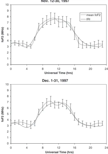
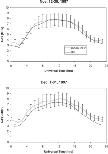
mid-latitudes, and Grahamstown, South Africa, in the Southern Hemisphere. Ionospheric F-region critical frequencies (foF2) have been obtained from the NOAA National Geophysical Data Center, Boulder. Figure 2 shows the monthly mean and standard deviations of the diurnal variation at Rome for the November and December data. Note that the monthly mean for November is calculated using data only from November 12 to the end of the month. Also shown are the predictions from the IRI, which in this case is a good approximation to the mean data. The variability is about 2 MHz during the day and about 1 MHz at night. The root mean square error (RMSE) of the IRI ®t to the mean diurnal variation is 9% for both November and December.
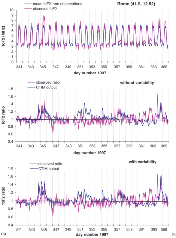
The top trace of Fig. 3a shows the observed foF2 at Rome relative to the monthly mean of the data, for the ®rst 25 days of the interval. The data shows little departure from the monthly mean during the minor disturbance during the ®rst 10 days, but is hampered by a lack of data during part of the interval. The data show a substantial increase above the mean during the larger event on November 23. The ratio between these two top traces is shown in red in the middle and lower
panels of Fig. 3a, together with the equivalent values from the two CTIM simulations. The simulation with-out variability is shown in the center, and the one with variability is shown in the lower panel. The model values are obtained by taking the ratio between the disturbed and quiet model runs. Note that the change in F-region peak electron density (NmF2), is the square of the foF2 ratios; a 40% increase in foF2 corresponds to a 96% increase in NmF2, indicating the ionospheric responses are quite substantial.
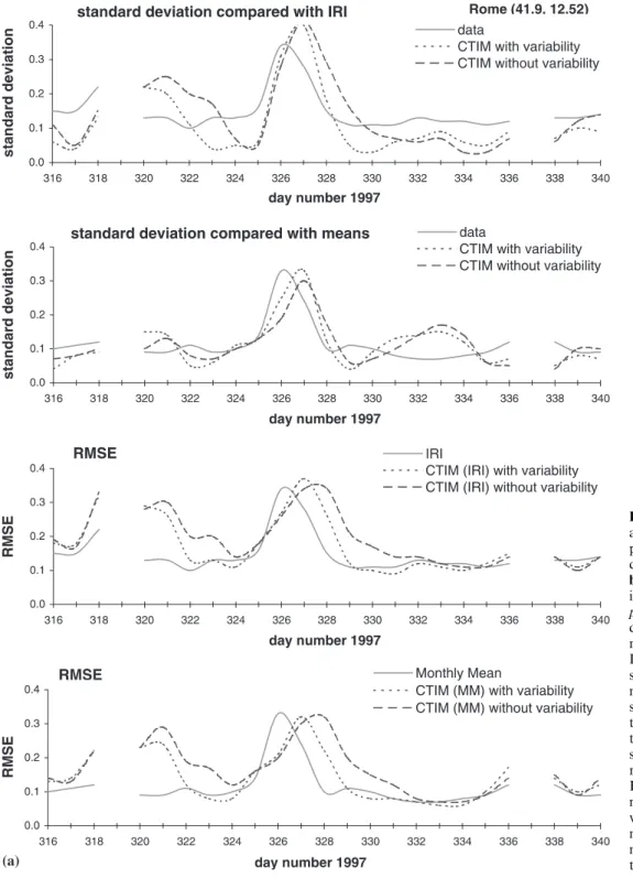
During the ®rst, small but prolonged disturbance, very little response is seen in the data. The model responses, the blue curves in the middle and lower panels, show a stronger positive tendency over this ®rst interval than is indicated in the data. Unfortunately, the data gap spoils a complete comparison. For the second, more major storm-like disturbance, the agreement of the model and data is very encouraging, particularly for the simulation with variability, in the lower panel. The ionospheric foF2 at Rome is seen to increase by about 50%, equivalent to more than a doubling in density, during the disturbance, and has been matched well by the model. The recovery of the data to background levels appears to be faster than both model simulations, although the data are matched slightly better when variability is included. The reason for this discrepancy in the rate of recovery may be partly due to the omission of self-consistent nitric oxide (NO). For these semi-opera-tional model runs, in the interest of computasemi-opera-tional speed, the self-consistent odd nitrogen chemistry was excluded. Maeda et al. (1989) showed that the rise in NO during a storm increases the cooling rate and hastens the recovery time of thermospheric temperature. To achieve a quantitative comparison, Fig. 4a illus-trates several statistical analyses. The standard devia-tions (SD) from the two model simuladevia-tions and the data for these ®rst 25 simulated days are displayed in the two upper panels of Fig. 4a. The SD is a measure of the level of the day-to-day variability, in other words how much the middle and lower model traces in Fig. 3a departs from unity. The values are calculated for each day using the 24 hourly values. The solid line in the top panel shows the SD of the data normalized by IRI; the SD of the ionospheric ratios from the two model simulations, with and without variability, are shown as dotted and dashed lines respectively. The second panel shows the data normalized by the monthly mean of the diurnal variation. The dierence in the line representing the data in the ®rst and second panels is small because the IRI was a good ®t to the mean diurnal variation, as was seen Figure 2. The SD of the model ratios in the second panel are not calculated from the actual ratios, as shown in Fig. 3a, but are the ratios relative to the monthly mean of the model ratios. From the model, the mean ratio for November was high by about 10 to 15%. Allowing for this shift in the mean model ratios explains the dierence in the ®rst and second panel. Note that in operational terms neither the monthly mean of the data nor the mean model ratios would actually be available; for the purposes of comparison, however, it is useful to include in the analysis.
Fig. 2. Mean and standard deviation of the diurnal variation of foF2 at Rome for November and December, 1997, together with the prediction from the International Reference Ionosphere
During the quiet intervals, the data ¯uctuates about the mean with about a 10% standard deviation. Surprisingly, both simulations have about the same standard deviation about the mean, and are in good agreement with the data. Inclusion of high-latitude electric ®eld variability does not appear to have much impact on the hour-to-hour ionospheric variability at mid-latitudes. The fact that the model reproduces the average variability in the data is surprising since the observations will respond to variability of the solar extreme ultraviolet radiation and upward-propagating waves, in addition to the geomagnetic sources. A recent CEDAR workshop estimated that each of these sources
contributes roughly equal amounts to the normal day-to-day variability of the ionospheric F region. The data, of course, also include instrumental noise, but these hand-scaled ionograms are expected to provide quality data with precision of better than 2% in foF2 or 4% in NmF2. During the storm interval, the standard devia-tion in the data increases to 30%, and the model simulation captures the magnitude of this increase well, but is a little late. Note the idea of predicting the increase in ionospheric variability during a storm can be valuable to an operational user.
In the third and fourth panels of Fig. 4a values for the daily root-mean-square (RMS) error are presented.
Fig. 3a, b. Comparison of the observed and modeled foF2 at Rome, for a the ®rst 25 days of the 50-day interval, and b the second 25 days of the 50-day interval. In each case, the top trace shows the observed foF2 in relation to the mean monthly diurnal variation. The ratio be-tween these two traces is shown in the middle panel, together with the value extracted from the CTIM model simulations without vari-ability. The lower panel shows the same data in comparison with the model simulation with variability
The third panel illustrates the RMS error using the IRI model to predict the data, together with the IRI values scaled by the model predicted ratios. In the fourth panel, the RMS error using the monthly mean is shown together with the values predicted by scaling the monthly mean by the normalized model ratios (as explained above for the second panel). During the quiet periods the RMS error of the physical model and the monthly mean are comparable. During the active period early in the 25-day interval, the physical model is worse. During the ®rst two days of the storm on November 22 and 23 the physical model does better than climatology,
but then is worse again during the recovery period, due to the slower recovery in the model. Note that IRI is not designed to capture changes resulting from increased geomagnetic activity. This ®rst quantitative comparison is a stark reminder of the diculty of improving on ionospheric predictions by empirical climatological models such as IRI. Although IRI does not capture the storm-time increase, at least it does not overestimate during the other times.
Figure 1b shows the geophysical condition for the second 25-day interval. The main features are a signi®-cant disturbance on day 345, December 11, where the
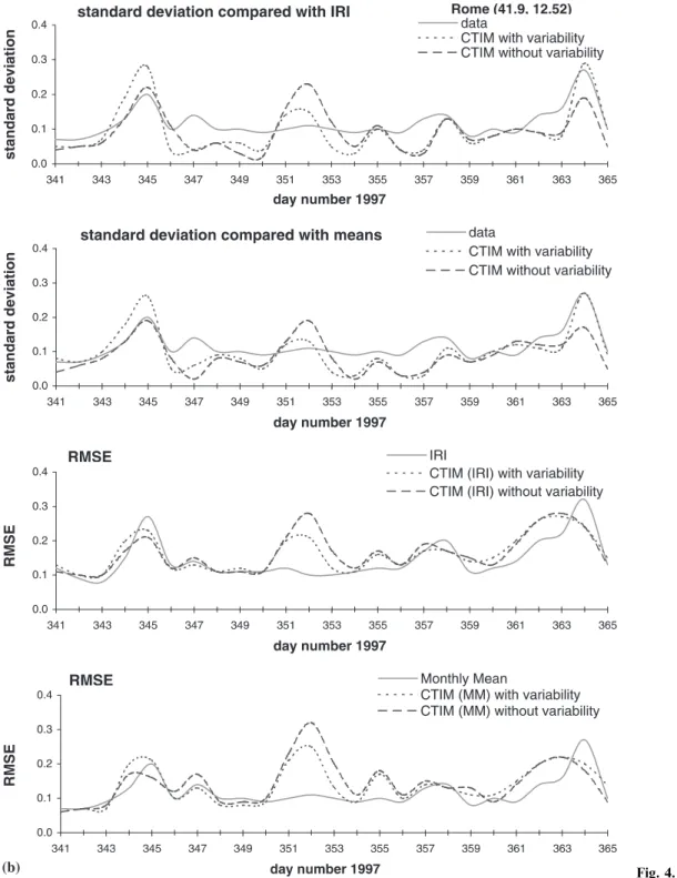
auroral power reached 150 GW, and the oval expanded 10°S, and then again on the penultimate day of 1997, when about the same level of disturbance was recorded. Figure 3b shows the same information as Fig. 3a, but for the second half of the 50-day interval. Similar conclusions can be reached during this period for both the quiet background levels and the two storm intervals. During the two disturbed intervals on days 344/345 and at the end of the year, the model and the data both show increases in foF2. The model tended to overestimate the foF2 on day 352 when there was a slight increase in geomagnetic activity but no response in the ionosphere
was detected. During the last few days in the year, the ionosphere also showed increases in the nightside that are not associated with geomagnetic activity. These increases may be associated with increases in EUV radiation.
The statistics for this second interval are shown in Fig. 4b. The standard deviation of the day-to-day variability in the model is again similar in the data, with increases to above 0.2 during the two storm periods for both the model and data. The model overestimated the response to the increase in activity on day 352, making it appear storm-like, although no increase was
Fig. 4a, b. Summary of statistical analysis of the model/data com-parison at Rome for a the ®rst 25 days of the 50-day interval, and b the second 25 days of the 50-day interval. In both cases, the top panel shows the daily standard deviation of the data and the two model simulations normalized by IRI, and the second panel is the same but normalized by the monthly mean. The third panel shows the RMS errors by using the IRI model to predict the data, together with the IRI values scaled by the model predicted ratios. In the fourth panel, the RMS error using the monthly mean is shown together with values predicted by scaling the monthly mean by the normalized model ratios (as explained in the text)
seen in the data. In the lower two panels, compared with IRI (third panel) or the monthly mean (fourth panel) the physical model was not able to make a signi®cant reduction in the RMS error, except perhaps for day 364. The ``false-alarm'' produced by the physical model on day 352, December 18, caused a large increase in the RMS error of the model. Compared to the visual comparisons in Fig. 3, the quantitative assessments are a little disappointing.
The second model/data comparison is with the Southern-Hemisphere station of Grahamstown, SA. Figure 5 shows the monthly mean and standard
devi-ations of the diurnal variation for November and December. Note that, as before, the averages for November are evaluated using data from November 12 to the end of the month. Also shown are the predictions from the IRI, which is a very good approximation to the mean data in November with a RMSE of 7%, but is consistently low in December with a RMSE of 15%. The Grahamstown data tends to be slightly more variable than Rome, particularly in November, with variability of about 3 MHz during the day and about 1.5 MHz at night. The cause of the larger variability in Grahamstown during November
most probably re¯ects geophysical processes rather than an increase in instrument noise or analysis problems. Some of the increase in variability comes from the departure of the dayside ionosphere from the mean during the last few days of the month, which is discussed further later. Summer mid-latitude data might be expected to be less variable due to higher neutral N2/O ratios, leading to stronger chemical control of the
ionosphere. Examination of the predictions by the physical model reveal that this is certainly the case in the simulations but is not re¯ected in the data. In winter, the large transient ¯uctuations in electron density are associated with wind surges that are captured by the model. In summer, it is possible that some of the variability is caused by structure in the neutral composition that is not present in the model. This composition structure could arise from coherent small-scale features in the Joule heating rate that are neither present in the statistical patterns nor are captured by the imposed variability.
The top trace of Fig. 6a shows the observed foF2 at Grahamstown compared with the monthly mean of the data, for the ®rst 25 days of the interval. The middle and lower parts of the ®gure shows the ratio of the data with
the monthly means, together with CTIM predictions from the two simulations, in the same format as was shown for Rome. During the prolonged disturbance during the early part of the interval, the data shows a long-lived reduction in foF2 by about 10 to 15% below the mean, which is followed well by both model simulations. During the stronger disturbance on day 327 and 328 the data drops sharply by about 30%. The model also shows depletions at this time, but with a slightly smaller magnitude; the simulation with variabil-ity matches the data better but both are a little slow to respond. Up to day 330, the model follows the data well and the comparison can be regarded as a success, and a vindication of our understanding of the physical pro-cesses. Towards the end of this ®rst 25-day interval, the Grahamstown data deviates signi®cantly from the mean, and from the model. This large and fairly consistent increase on the dayside lasts for several days from day 331 and is during a period of geomagnetic quiet. The explanation could arise from changes in the solar ¯ux, since data from the SOHO spacecraft indicate a rise in EUV ¯ux during this time (R. Viereck, private commu-nication). The magnitude of the EUV increase, and the consequent change in the ionosphere, has yet to be compared quantitatively. The question also arises as to why the summer hemisphere should respond to this possible change in EUV, but the winter station at Rome does not.
In Fig. 7a, the statistics for Grahamstown are presented for the ®rst 25-day interval. The format of the four panels are the same as in Fig. 4 for Rome, with standard deviations shown in the top two panels and RMS errors in the lower panels. Except for the last ten days of the interval that are dominated by the possible EUV increase, the day-to-day SD of the data are a little higher than for Rome. The model SD is generally lower, but the storm-time increases are reasonably consistent with the data albeit with smaller magnitudes. The RME errors from the model for Grahamstown perform better than for Rome, largely due to the absence of false alarms. During the quiet periods, the model performs about the same as IRI. The model reduces the data variance a little during the disturbances, but the improvements are small.
During the second 25-day interval for Grahamstown (Fig. 6b) the interpretation and conclusions are similar. The statistics for the second period at Grahamstown are shown in Fig. 7b. The SD in the model is low, but does show the increase during the disturbance on day 345, with reduced magnitude. For the RMS error statistics the physical model performs about the same as IRI, and does not produce any false alarms. A slight improve-ment relative to the monthly mean is apparent on day 345.
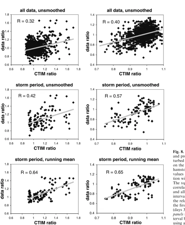
To complete the quantitative statistical analysis the relationship between the model predictions, with vari-ability, and data are presented for six cases in Fig. 8. The top two panels show the correlation between all the hourly data and the model predictions from the 50-day interval, with Rome on the left, and Grahamstown on the right. For Rome, the correlation coecient is only
Fig. 5. Mean and standard deviation of the diurnal variation of foF2 at Grahamstown, South Africa, for November and December, 1997, together with the prediction from the International Reference Ionosphere
0.32, and for Grahamstown, the model performance is slightly better with a correlation coecient of 0.4. Neither is a resounding vindication of the model or of our understanding of the physical processes of the ionospheric response to geomagnetic activity. This comparison with all data, unsmoothed, is perhaps a little unfair since it is mostly the hour-to-hour variability that is being tested. The model is expected to capture the magnitude of the variability but is not expected to capture the phase of every wiggle in the data.
Correla-tion coecients are a measure of the ability to match the phase in a signal. A fairer test of the model is to select the storm intervals for the comparison. The middle two panels show the relationship between the data during days 325 to 329 covering the ®rst major storm interval, for the two sites. The correlation coecient has increased to 0.42 for Rome and 0.57 for Grahamstown. Finally, the lower panels show the same interval but with the data smoothed using a ®ve point running mean, to remove some of the hour-to-hour variability. The
Fig. 6a, b. Same as Fig. 3 but for Grahamstown
correlation coecients now increase to about 0.65 for both sites, a signi®cant improvement, although still not a resounding success. The gradient of the linear ®t in the scatter plot is a measure of the sensitivity of the model ionosphere to geomagnetic activity. In Grahamstown the gradient (model/data) for the smoothed storm interval is 0.8, implying that the model response to geomagnetic activity is, on average, 80% of the observed response. In Rome, due to the slow recovery of the modeled ionosphere, the gradient (model/data) is 2.0, implying an overestimate of the model response by a factor of two. During the rising phase of the storm to
the peak in the ionospheric response at Rome, the overestimate is smaller (1.4), which is more consistent with the visual inspection of Fig. 3a.
5 Discussion and conclusions
Historical data (Rodger et al., 1989) and recent theo-retical studies (Fuller-Rowell et al., 1996) indicate that the ionospheric response to a geomagnetic storm in winter and summer mid-latitudes is very dierent. Rodger et al., (1989) showed that at a southern
magnetic mid-latitude station a consistent local-time signature in the ratio of disturbed-to-quiet NmF2 existed throughout the year, with a minimum in the morning hours around 06 LT, and a maximum in the evening hours around 18 LT. The local-time ``AC'' variation was superimposed on a ``DC'' shift of the mean level that varied with season, being most positive in winter (May± July) and most negative in summer (October±February). The data support the widely held belief that positive storms are more likely in winter mid-latitudes and negative storms more likely in summer. Fuller-Rowell et al., (1996) suggested an explanation of the seasonal
variations. Numerical computations showed that the prevailing summer-to-winter circulation at solstice transports the molecular-rich gas to mid- and low latitudes in the summer hemisphere over the day or two following the storm. In the winter hemisphere, poleward winds restrict the equatorward movement of composition. The altered neutral-chemical environment in summer subsequently depletes the F-region mid-latitude ionosphere to produce a negative phase. In winter mid-latitudes, a decrease in molecular species, associated with downwelling, persists and produces a positive phase.
Fig. 7a, b. Same as Fig. 4 but for Grahamstown
A 50-day interval at the end of 1997 has been simulated with a coupled thermosphere ionosphere model to test our understanding of the physical processes controlling the upper atmospheric response to geomagnetic storms, and to determine the value of model predictions for space weather applications. The model has been validated by comparing with two mid-latitude ionosonde stations in the northern winter hemisphere and southern summer hemisphere. The visual comparisons between model and data support our current understanding of the physics, and clearly show that the model is able to capture the general
magnitude and seasonal character of the storm-time ionospheric response. The simulation with electric ®eld variability included tended to perform better. From these visual comparisons, one would conclude that we have a reasonable understanding of the physical mech-anisms, and the model/data comparisons shown in Figs. 3 and 6 can be regarded as a modeling success.
For space weather applications, the value of a model prediction must go beyond visual comparison to a more quanti®ed measure of success. This has been done by evaluating the model performance using three dierent metrics: the magnitude of the daily standard deviation,
the RMS error, and the correlation coecient. In spite of the clear science merit of the physical modeling, the results of the quantitative comparisons are not very encouraging. The physical model reproduces the mag-nitude of the day-to-day variability in the data in winter (10% in foF2), and follows the increase in variability during the storm (30% in foF2). In summer mid-latitudes, the model tends to underestimate the day-to-day variability, and the magnitude of the negative phase. Using the model predictions, the RMS errors are improved only during part of the storm interval com-pared with IRI or the monthly mean, reducing the peak value of 0.3 to about 0.2 during the storm on November 22/23. At other times the physical model performs about
the same as climatology, except during the recovery to the storm at Rome, and during an earlier active period, when the physical model performance is not as good as climatology.
In terms of the correlation coecients, using un-smoothed data over the full interval the correlation coecients are low, between 0.3 and 0.4. Isolating the storm intervals increases the correlation to between 0.43 and 0.57, and by smoothing the data the values increases up to 0.65. These values re¯ect our current ability to predict the ionosphere during storms rather than our knowledge of the physical processes. One of the key conclusions of this work is that scienti®c merit and space weather success are quite dierent; scienti®c success is
Fig. 8. Correlation of observed and predicted ratio of the dis-turbed to quiet foF2, for Rome, on the left-hand side, and Gra-hamstown on the right.The model values are taken from the simula-tion with electric ®eld variability. The top two panels show the correlation between the model and all the data over the 50-day interval, the middle panels show the relationship between during the ®rst major storm interval (days 325 to 329), and the lower panels show the same storm in-terval but with the data smoothed using a ®ve point running mean
not sucient in de®ning operational value. This may indicate the state of ionospheric modeling, or more likely re¯ects how dicult it is to model the response at a particular station to a speci®c disturbance. This was shown by Codrescu et al. (1997), who demonstrated that one of the big limitations to upper atmospheric model-ing is the accuracy with which the high-latitude forcmodel-ing is de®ned. Uncertainty in the magnitude and spatial distributions of the magnetospheric electric ®eld and auroral precipitation can make a big dierence in the response at a particular site. More accurate speci®cation of the model drivers is necessary to improve the predictions and eliminate the false alarms.
Acknowledgements. This work was supported by the National Science Foundation grant ATM-9713440. The authors thank Eduardo Araujo-Pradere for help in preparing the ®gures.
Topical Editor M. Lester thanks M. FoÈrster and another referee for their help in evaluating this paper.
References
Anderson, D. N., M. J. Buonsanto, M. Codrescu, D. Decker, C. G. Fesen, T. J. Fuller-Rowell, B. W. Reinisch, P. G. Richards, R. G. Roble, R. W. Schunk, and J. J. Sojka, Intercomparison of physical models and observations of the ionosphere, J. Geophys. Res., 103, 2179±2192, 1998.
Burns, A. G., T. L. Killeen, and R. G. Roble, A theoretical study of thermospheric composition perturbations during an impul-sive geomagnetic storm, J. Geophys. Res., 96, 14 153±14 167, 1991.
Burns, A. G., T. L. Killeen, W. Deng, and G. R. Carignan, Geomagnetic storm eects in the low to middle-latitude upper thermosphere, J. Geophys. Res., 100, 14 673±14 691, 1995. Codrescu, M. V., T. J. Fuller-Rowell, and J. C. Foster, On the
importance of E-®eld variability for Joule heating in the high-latitude thermosphere, Geophys. Res. Lett., 22, 2393±2396, 1995.
Codrescu, M. V., T. J. Fuller-Rowell, and I. S. Kutiev, Modeling the F layer during speci®c geomagnetic storms, J. Geophys. Res., 102, 14 315±14 329, 1997.
Codrescu, M. V., T. J. Fuller-Rowell, and J. C. Foster, Small-scale variability in the ionospheric convection pattern, AGU Spring Meeting, Boston, 1998.
Codrescu, M. V., T. J. Fuller-Rowell, J. C. Foster, J. M. Holt, and S. J. Cariglia, Electric ®eld variability associated with Mill-stone Hill electric ®eld model, J. Geophys. Res., 105, 5265±5273, 2000.
Emery, B. A., et al., Assimilative mapping of ionospheric electro-dynamics in the thermosphere-ionosphere general circulation model comparisons with global ionospheric and thermospheric observations during the GEM/SUNDIAL period of March 28± 29, 1992, J. Geophys. Res., 101, 26 681, 1996.
Foster, J. C., J. M. Holt, R. G. Musgrove, and D. S. Evans, Ionospheric convection associated with discrete levels of particle precipitation, Geophys. Res. Lett., 13, 656, 1986.
Fuller-Rowell, T. J., and D. Rees, A three-dimensional, time-dependent, global model of the thermosphere, J. Atmos. Sci., 37, 2545, 1980.
Fuller-Rowell, T. J., and D. S. Evans, Height-integrated Pedersen and Hall conductivity patterns inferred from the TIROS-NOAA satellite data, J. Geophys. Res., 92, 7606, 1987. Fuller-Rowell, T. J., S. Quegan, D. Rees, R. J. Moett, and
G. J. Bailey, Interactions between neutral thermospheric composition and the polar thermosphere using a coupled global model, J. Geophys. Res., 92, 7744, 1987.
Fuller-Rowell, T. J., M. V. Codrescu, R. J. Moett, and S. Quegan, Response of the thermosphere and ionosphere to geomagnetic storms, J. Geophys. Res., 99, 3893±3914, 1994.
Fuller-Rowell, T. J., M. V. Codrescu, R. J. Moett, and S. Quegan, On the seasonal response of the thermosphere and ionosphere to geomagnetic storms, J. Geophys. Res., 101, 2343±2353, 1996. Fuller-Rowell, T. J., M. V. Codrescu, R. G. Roble, and A. D. Richmond, How does the thermosphere and ionosphere react to a geomagnetic storm, AGU Geophysical Monograph 98 on Magnetic Storms, 203±225, 1997.
Kamide, Y., W. Sun, and S.-I. Akasofu, The average ionospheric electrodynamics for the dierent substorm phases, J. Geophys. Res., 101, 99±109, 1996.
Maeda, S., T. J. Fuller-Rowell, and D. S. Evans, Zonally averaged dynamical and compositional response of the thermosphere to auroral activity during September 18±24, 1984, J. Geophys. Res., 94, 16 869, 1989.
ProÈlss, G. W., Common origins of positive ionospheric storms at middle latitudes and the geomagnetic eect at low latitudes, J. Geophys. Res., 98, 5981±5991, 1993.
ProÈlss, G. W., Storm-induced changes in the thermospheric composition at middle latitudes, Planet. Space Sci., 35, 807± 811, 1987.
ProÈlss, G. W., Magnetic storm perturbations of the upper atmosphere, AGU Geophysical Monograph 98 on Magnetic Storms, 227±241, 1997.
ProÈlss, G. W., S. Werner, M. V. Codrescu, T. J. Fuller-Rowell, A. G. Burns, and T. L. Killeen, The thermosphere-ionosphere storm of December 8, 1982: model predictions and observa-tions, Adv. Space Res., 22, 123±128, 1998.
Rishbeth, H., T. J. Fuller-Rowell, and A. D. Rodger, F-layer storms and thermospheric composition, Phys. Scripta, 36, 327±336, 1987.
Rodger, A. S., G. L. Wrenn, and H. Rishbeth, Geomagnetic storms in the Antarctic F region, II, physical interpretation, J. Atmos. Terr. Phys., 51, 851±866, 1989.
Quegan, S., G. J. Bailey, R. J. Moett, R. A. Heelis, T. J. Fuller-Rowell, D. Rees, and R. W. Spiro, Theoretical study of the distribution of ionization in the high-latitude ionosphere and the plasmasphere: ®rst results on the mid-latitude trough and the light ion trough, J. Atmos. Terr. Phys., 44, 619, 1982. Wrenn, G. L., A. S. Rodger, and H. Rishbeth, Geomagnetic storms
in the Antarctic F region. I. Diurnal and seasonal patterns for main phase eects, J. Atmos. Terr. Phys., 49, 901±913, 1987.