The annual cycle of hydrogen peroxide: is it an indicator of chemical instability?

(1)

HAL Id: hal-00301176

https://hal.archives-ouvertes.fr/hal-00301176

Submitted on 6 Apr 2004

HAL is a multi-disciplinary open access

archive for the deposit and dissemination of sci-entific research documents, whether they are pub-lished or not. The documents may come from teaching and research institutions in France or abroad, or from public or private research centers.

L’archive ouverte pluridisciplinaire HAL, est destinée au dépôt et à la diffusion de documents scientifiques de niveau recherche, publiés ou non, émanant des établissements d’enseignement et de recherche français ou étrangers, des laboratoires publics ou privés.

The annual cycle of hydrogen peroxide: is it an indicator

of chemical instability?

R. W. Stewart

To cite this version:

R. W. Stewart. The annual cycle of hydrogen peroxide: is it an indicator of chemical instability?. Atmospheric Chemistry and Physics Discussions, European Geosciences Union, 2004, 4 (2), pp.1941-1975. �hal-00301176�

(2)

ACPD

4, 1941–1975, 2004 Hydrogen peroxide and chemical instability R. W. Stewart Title Page Abstract Introduction Conclusions References Tables Figures J I J I Back Close

Full Screen / Esc

Print Version Interactive Discussion

Atmos. Chem. Phys. Discuss., 4, 1941–1975, 2004 www.atmos-chem-phys.org/acpd/4/1941/

SRef-ID: 1680-7375/acpd/2004-4-1941 © European Geosciences Union 2004

Atmospheric Chemistry and Physics Discussions

The annual cycle of hydrogen peroxide: is

it an indicator of chemical instability?

R. W. Stewart

NASA Goddard Space Flight Center, Greenbelt, MD 20771, USA

Received: 11 March 2004 – Accepted: 25 March 2004 – Published: 6 April 2004 Correspondence to: R. W. Stewart (richard.w.stewart@nasa.gov)

(3)

ACPD

Full Screen / Esc

Abstract

A box model has been used to study the annual cycle in hydrogen peroxide concen-trations with the objective of determining whether the observed difference in summer and winter values reflects instability in the underlying photochemistry. The model is run in both steady-state and time-dependent modes. The steady-state calculations

5

show that, for some range of NO_x background levels, two stable solutions to the con-tinuity equations exist for a period of days in spring and fall. The corresponding time-dependent model indicates that, for sufficiently high background NO_x concentrations, the spring and fall changes in H₂O₂concentration may be interpreted as a forced tran-sition between the two underlying stable regimes. The spring trantran-sition is more rapid

10

than that in fall, an asymmetry that becomes more marked as background NO_x in-creases. This asymmetry is related to the different time scales involved in chemical production and loss of H₂O₂. Observations of the spring increase in H₂O₂ concentra-tion may therefore provide a better measure of the change in the underlying chemical regime than does the fall decrease.

15

1. Introduction

Several publications (e.g. White and Dietz, 1984; Stewart, 1993; Kleinman, 1994) have shown that the continuity equations that describe tropospheric photochemistry can ex-hibit bifurcations and consequent multiple steady-state solutions. These phenomena occur in the transition region between what may be characterized as low-NO_x and

20

high-NO_x chemical regimes. It is not known whether these mathematical properties exhibited by steady-state models correspond to observable phenomena in the time-dependent world. This paper addresses the question of observable consequences.

Steady-state and time-dependent calculations over an annual cycle are carried out showing that bifurcations in the steady-state solutions have an analogue in the

time-25

(4)

con-ACPD

Full Screen / Esc

centrations occur in time-dependent calculations. These correspond to bifurcations in the steady-state case. The rapidity of the transition increases with increasing back-ground NO_x.

It is obvious that such transitions do not occur on the global scale, a predominately low-NO_x environment. Their importance lies in the fact that, should they occur on

5

more polluted regional scales, they can involve large changes in oxidant levels with a corresponding change in pollutants over a short time period of several days. Hydrogen peroxide, the focus of the discussion in this paper is an especially sensitive indicator of the low-NO_x, high-NO_xtransition.

1.1. The observed annual cycle of H₂O₂

10

This paper will discuss the annual cycle of H₂O₂ in the context of the low-NO_x and high-NO_x chemical regimes described by Kleinman (1991). A basic difference in these regimes is the concentration and fate of oxidants. In the high-NO_x regime OH reacts predominantly with NO₂to form nitric acid. Nitric acid is mostly removed by deposition before it can react to return its components to the atmosphere and its formation is thus

15

a permanent loss for odd hydrogen (HO_x=OH+HO₂). Since H₂O₂ is formed through reaction of two HO₂radicals it is particularly sensitive to the changes in concentration of HO_x components that occur in the transition from low-NO_x to high-NO_x conditions. We will explore the possibility that observed mixing ratio changes in the tropospheric boundary layer might, under some circumstances, be interpreted as resulting from

20

instability in the underlying steady-state chemistry. Due to the sensitivity of hydrogen peroxide to such instability it is reasonable to concentrate on its annual cycle.

Most measurements of H₂O₂have been made over relatively limited time spans (see the review by Lee et al., 2000). Measurements over an annual cycle have been made by Ayers et al. (1996) at Cape Grim, Tasmania (41◦S) and Sakugawa and Kaplan

25

(1989) in and near Los Angeles, CA. The Ayers et al. (1996) measurements represent unpolluted marine air and show monthly means varying from 0.16 to 1.4 ppb. The measurements of Gnauk et al. (1997) were carried out over a 3-year period, but are

(5)

ACPD

Full Screen / Esc

only reported for selected days or over short intervals. Peroxide observations were made over a four-month period during the Tropospheric Ozone Production about the Spring Equinox (TOPSE) experiment (Snow et al., 2003). Although this time period is of special interest to the present study, the NO_xmixing ratios were too low to contribute to low to high-NO_xtransitions (Snow et al., 2003; Tie et al., 2003).

5

The body of observations covers different locations and times of year and is useful for deducing general characteristics of the annual cycle of H₂O₂. The property of the H₂O₂ annual cycle of most interest in this study is the change from a winter minimum to a summer maximum under various levels of background pollution as represented by the NO_x mixing ratio.

10

1.2. Nonlinearities

The nonlinearity of the continuity equations describing various aspects of atmospheric photochemistry gives rise to a number of interesting consequences. This paper will focus on multiple solutions in tropospheric models, but these have also been discussed with regard to the stratosphere (Prather et al., 1979; Fox et al., 1982; Konovalov et al.,

15

1999) and mesosphere (Yang and Brasseur, 1994).

A relatively simple consequence of nonlinearity that has been discussed in the con-text of tropospheric models for some time is ’turnaround’ behavior. This refers to a change in sign of the rate of change of a species concentration, such as ozone, with respect to a monotonically changing control parameter, such as a nitric oxide

20

source. Stewart et al. (1977) described the change in O₃ response with increasing NO_xemission. They showed that [O₃] first increased, then decreased as NO emission increased, with a turnaround occurring when the NO_x background reached roughly 500 ppt. Hameed et al. (1979) discussed the importance of the NO_x background on OH behavior and on the effect of increased CO source levels in the troposphere. The

25

hydroxyl radical, like ozone, exhibits a turnaround as we go from a low to a high-NO_x background. It was shown that an increasing CO source could either increase OH and decrease CH₄or have the opposite effect as NO_x background changes. Poppe et

(6)

ACPD

Full Screen / Esc

al. (1993) discussed the nonlinear OH response to changes in several model parame-ters.

White and Dietz (1984) were the first to describe a more startling aspect of nonlin-earity in a tropospheric model, the existence of multiple steady states. These authors showed that the NO_x removal rate is a non-monotonic function of NO_x concentration.

5

This implies that multiple concentration values can exist for each NO_x source value within a specific range of NO_x emission rates. Stewart (1993, 1995) described meth-ods for computing multiple solutions and exhibited them for a variety of assumptions regarding both the reactions included in a model and the source values for key species. Multiple solutions occur when a control parameter, typically NO source, is varied past a

10

critical value at which a bifurcation from one to three solutions occurs. Further variation in the same direction leads to another bifurcation in which the number of solutions is re-duced to one. These bifurcation points bound a bistable region in the state space of the system, i.e. a region in which two stable steady states exist. It has not been clear how, or if, the bistability exhibited in simple models relates to observable phenomena.

Klein-15

man (1991) suggested that the difference in summer and winter H₂O₂concentrations observed in the northeastern United States might reflect the difference in underlying low-NO_x (summer) and high-NO_x (winter) photochemical states. Jacob et al. (1995) suggest that measurement of H₂O₂, and several other species, show evidence of a September transition from low-NO_x (NO_x-limited) to high-NO_x (hydrocarbon-limited)

20

conditions. Their data, along with other observations noted in the paper, suggest a roughly factor of 5 decrease in H₂O₂during September.

1.3. Chemical instability

The terms “chemical instability” and “unstable solution” are used throughout this paper. Both steady-state and time-dependent solutions of continuity equations are presented

25

to illustrate the phenomena described by these terms and possible atmospheric con-sequences of such phenomena. For corresponding parameter values, the steady-state solutions are expected to serve as “attractors” for the time-dependent model. For

(7)

exam-ACPD

Full Screen / Esc

ple, the solutions of a diurnally forced model should remain close to the corresponding solutions of a diurnally averaged one. In this sense, steady state models can provide an approximation to averaged conditions in the atmosphere. An exception occurs if the steady-state solution is unstable.

An unstable solution refers to a steady-state model in which the Jacobian matrix,

5

evaluated at a solution, has at least one eigenvalue with a positive real part. The Newton-Raphson method used in solving the steady-state model (Stewart, 1993) uses the Jacobian, but not its eigenvalues. In a steady-state model there is thus no com-putational difference between stable and unstable solutions. If we now solve the same equations, but use a time-dependent method to study the behavior of the solutions

10

near a steady state, the Jacobian eigenvalues appear as arguments of exponential functions that describe the model’s temporal evolution. If the real parts of all eigen-values are negative, the solution simply relaxes to the steady state, but any positive real part will drive the time-dependent solution away from the steady state. This is the meaning of instability and the consequence is that unstable steady-state solutions

15

are inaccessible to a time-dependent model and cannot provide an approximation to conditions in the atmosphere.

Our interest in instability is in determining how a time-dependent model behaves when underlying steady-state attractors, differing only by a small value of a parameter, are nonetheless widely separated in the state space of the system. This will occur in

20

bistable regions referred to above. An example in the following is provided by steady states calculated at noon on successive days of the year. The small change in solar zenith angle that this entails will, under some conditions, result in large changes in species concentrations. When these steady-state changes have a time-dependent analog we expect that, to the extent that the time-dependent model provides some

25

(8)

ACPD

Full Screen / Esc

2. Background

2.1. Tropospheric chemical regimes

In both stratosphere and troposphere the source of ozone is molecular oxygen. In the stratosphere a single UV photon having wavelength λ≤242 nm suffices to dissociate molecular oxygen and form O₃via reaction of the product O atoms with O₂. Since these

5

photons do not penetrate to the troposphere, ozone production utilizes two less ener-getic photons and a more involved sequence of chemical reactions. The first photon,

λ≤340 nm, photolyzes a seed molecule of O₃ yielding an excited-state oxygen atom, O(1D). This may then react with water vapor to form OH. OH oxidation of a hydrocar-bon (HC), represented by CO and CH₄ in the following, releases H atoms or methyl

10

radicals, respectively. These capture O₂ to form HO₂ or CH₃O₂ and, with sufficient NO present, an O atom is subsequently transferred to NO forming NO₂. The second photon, λ≤423 nm, now photolyzes NO₂releasing O to form O₃as in the stratosphere. Since this process only consumes HC and H₂O and not NO_x or HO_x there is no need for further O₃ photolysis to continue O₃production. Ozone in the troposphere is thus

15

its own precursor and its production is autocatalytic (Stewart, 1995). These ideas are elaborated in the remainder of this section.

A simplified photochemical scheme will be used to illustrate the behavior of the model used in this study. Such a simplification is often used to demonstrate basic properties of tropospheric chemistry and variants have appeared often in the literature (Tinsley and

20

Field, 2001; Field et al., 2001; Kalachev and Field, 2001; Prather, 1994). The actual model chemistry is described later, but the simplified scheme will be a useful reference for interpreting model results and understanding conditions in which bifurcations in the steady-state model and low-NO_x, high-NO_x transitions in the time-dependent model occur. Many authors have discussed the reactions described below (e.g. Levy, 1971;

25

Crutzen and Zimmermann, 1991; Kleinman, 1991; Lelieveld et al., 2002).

The photochemical system may be regarded as consisting of three sets described as follows: 1) Initiation, 2) Chain propagation, and 3) Termination. The initiation phase

(9)

ACPD

Full Screen / Esc

begins with the photolysis of an ozone molecule by solar UV radiation in the 300– 340 nm range. This produces excited-state O(1D) atoms, some of which react with water vapor to form two OH radicals. These initial reactions may result in ozone loss or production, depending on subsequent reactions.

2.1.1. Initiation

5

O₃+ hν → O(1D)+ O₂ (R1)

O(1D)+ H₂O → 2OH. (R2)

The fate of oxidants after the initiation phase begins with oxidation of CO. Carbon monoxide serves here as a surrogate for CH₄ and other hydrocarbon species. Since NO_x and HO_x are not consumed in the following they are referred to collectively as

10

chain propagation reactions. 2.1.2. Chain propagation CO+ OH + O₂→ HO₂+ CO2 (R3) HO₂+ NO → NO₂+ OH (R4a) HO₂+ O₃→ OH+ 2O2 (R4b) 15 NO₂+ O₂+ hν → NO + O₃. (R5)

For simplicity only the following chain termination reactions are considered. 2.1.3. Termination

OH+ NO₂+ M → HNO₃+ M (R6)

HO₂+ HO₂→ H₂O₂+ O₂. (R7)

(10)

ACPD

Full Screen / Esc

In a low-NO_xregime the net chemistry may result in either ozone loss or production. If it results in production, large numbers of ozone molecules may be produced for each one initially photolyzed. Depending on the amount of CO or hydrocarbon (HC) available reactions (R3)–(R5) may occur several times before a termination reaction occurs that removes radicals or NO_xfrom the system. Suppose that reactions (R3)–(R5) occur m

5

times before a termination reaction occurs. Further, within this sequence, suppose that reaction R4a occurs m₁times and (R4b) m₂times with m₁+m₂=m. Then the net effect of (R1)–(R5) is:

2.1.4. Net

O₃+ H₂O+ mCO + (2m₁−m₂−1)O₂→ mCO₂+ 2OH + (m₁−m₂)O₃. (R8)

10

The above system behaves in the following way:

– Net production of O₃: m₁>m₂+1

– O₃neutral: m₁=m₂+1

– Net destruction of O₃: m₁<m₂+1.

The transition from ozone destruction to ozone production in the low-NO_x regime

15

occurs when the reaction rates (R4a) and (R4b) are approximately equal, i.e. k_4b[O₃]=k_4a[NO].

Once there is sufficient NO in the system to provide net chemical production, we see from the net reaction that this production is autocatalytic with m₁–m₂ozone molecules produced for each one destroyed. For CH₄or NMHC consumption, the potential ozone

20

production is greater, but details will not be considered here.

Dominance of (R4b) over (R4a), if it occurs, does not imply that HO₂+O₃ is itself a major ozone loss mechanism. The competition between O₃ and NO for HO₂ simply provides a switch that, if O₃ is favored, allows ozone photolysis to act as the princi-pal ozone loss mechanism rather than as the first step in the autocatalytic production

(11)

ACPD

Full Screen / Esc

of ozone. This process was described as inhibition (of ozone production) in Stewart (1995).

The effects of these reactions are summarized in Fig. 1. The circles represent species playing the role of sources (HC) or sinks (H₂O₂ and HNO₃) for the more re-active species shown in the boxes. In this figure, the light-blue boxes and circles and

5

dark-blue arrows indicate the chemistry of the low-NO_x, ozone loss regime. OH produc-tion through reacproduc-tions (R1) and (R2) is followed by conversion to HO₂via hydrocarbon oxidation and then loss of HO_x and O₃ after reaction (R7) forms peroxide. The path (R3) followed by (R7) shows the loss of ozone and odd hydrogen. Net production of oxidants does not occur in this system.

10

Adding NO_x to the system provides the mechanism for autocatalytic production of ozone. This is shown by adding the brown boxes and green arrows in Fig. 1. The dotted green arrows in the diagram show the recycling of NO_x and HO_x. The arrows connected to small filled circles in the HO₂ box indicate the alternate pathways that may be followed by HO₂. The low-NO_x switch from ozone loss to production occurs

15

when the (R4a) path dominates (R4b) as described above.

Finally, when enough NO_xis present, OH will react preferentially with NO₂to form ni-tric acid. This establishes the high-NO_xregime shown by adding the red circle (HNO₃) and arrows on the left side of Fig. 1. Once this occurs the low-NO_x paths on the right of the figure are substantially shut down and production of oxidants, including H₂O₂,

20

becomes negligible. The small filled circles in the OH box indicate the switch between low and high-NO_xchemistry.

2.2. Model description

2.2.1. Methods and parameters

Many model details are the same as described in Stewart (1993, 1995). A box model

25

(Stewart et al., 1983) is used to compute species concentrations. A Newton-Raphson method (Press et al., 1992), modified to enhance its robustness (Stewart, 1993), is

(12)

ACPD

Full Screen / Esc

used to compute steady-state solutions and the LSODE integrator (Hindmarsh, 1983) is used for time-dependent runs. Methane is held fixed at a mixing ratio of 1.7 ppm. Temperature is assumed to vary through the year from 273K to 297K similar to the model of Kleinman (1991). Water vapor varies with an annual cycle consistent with the temperature change and the assumption of a fixed 60% relative humidity. Fixed ozone

5

burdens of 300 D.U. and boundary layer height of 1 km. have been used in the results reported below. Test calculations have been made with annual variations of these last parameters, but without significant change in the results.

There are 26 variable species (Table 1) undergoing 65 reactions (Table 2). In addi-tion to their chemical interacaddi-tions, several species shown in Table 1 are assumed to

10

have physical sources and/or sinks. The physical source of O₃ is transport from the stratosphere. The mean value used for the O₃flux is in the range discussed by Holton and Lelieveld (1994). The CO source is based on a global anthropogenic source value (Olivier et al., 1999). Sources for ethene and ethane are assumed that give values of these species consistent with observations (Bottenheim and Shepherd, 1995) over

15

some range of model runs. Except for H₂CO, deposition velocities are from the model study of Hauglustaine et al. (1994). The formaldehyde deposition rate is assumed the same as that for CH₃CHO.

Some experimentation has been carried out with all of these model parameters. The main qualitative features discussed below, namely the existence of spring and fall

tran-20

sitions between high and low-NO_x regimes in both steady-state and time-dependent models, have not been sensitive to the values used.

2.2.2. Chemistry

Table 2 presents the chemical reactions used in this study. Photolysis rates are com-puted from the Madronich (1987) model for clear sky conditions at 40◦N. Reaction

25

rates are mostly taken from Demore et al. (1997) and Atkinson et al. (1992). A few tests were made with updated values given in the compilation of Sander et al. (2003) with no significant change in results. Some of the reactions in Table 2 have products

(13)

ACPD

Full Screen / Esc

that react with O₂. In such cases, the products shown are those subsequent to the O₂ reaction. Reaction 1 showing ozone yielding OH directly is a composite reaction having an effective rate coefficient that depends on water vapor concentration as well as total number density. The effective rate is similar to that discussed in Stewart (1995), but is now treated as a photolysis rate rather than a bimolecular rate involving H₂O.

Hy-5

drolysis of N₂O₅(R41 in Table 2) follows the discussion of Dimitroulopoulou and Marsh (1997) using an effective rate that accounts for both heterogeneous and homogeneous reactions. Reactions (R50) and (R51) following the oxidation of C₂H₄by OH (R49) are based on the oxidation sequence given in Barker (1995). The rate for (R50) is a guess taken to be of a magnitude similar to the rates for HO₂+NO and CH₃O₂ + NO. The

10

thermolysis rate for (R51) is also a guess taken to be the same as the rate for HNO₄ thermolysis. The reactions (R52) and (R53) are based on Barker (1995) as well as the discussion of Paulson (1995).

3. Results

3.1. The computed annual cycle of H₂O₂

15

The primary control parameter in this study is the day of the year. Steady-state concen-trations for the variable species given in Table 1 are calculated at noon on successive days throughout the year. This implies a corresponding small variation in solar zenith angle between runs and it is also reasonable to consider zenith angle as the primary control parameter. Noon photolysis rates are multiplied by the daylight fraction for each

20

day to make the results more representative of diurnal averages obtained from a time dependent model than are noon values. The secondary control parameter is the ni-tric oxide source, S_NO. A range of source fluxes from 4×109 to 4×1012cm−2 s−1 has been used in the calculations. These are converted to source values by dividing by the boundary layer height (1 km). A time-dependent model has been run for a

two-25

(14)

ACPD

Full Screen / Esc

steady-state model. The annual cycles of H₂O₂from the steady-state model and from the second year of the time-dependent model are compared in this section.

In panels (c) and (d) of the following Figs. 2–5, the displayed rates of OH and HO₂ reaction are keyed to the discussion in Sect. 2.1 and the mechanism shown in Fig. 1. In some cases, at the higher NO_x levels, the formation of nitrous or pernitric acid is

5

actually among the top three rates. Rapid photolysis or thermolysis however will make these “do nothing” reactions and their exclusion is justified. In the models displayed in the following figures, reaction of OH with NMHC is not competitive with the rates shown.

Figure 2 shows steady-state calculations (a), the corresponding time-dependent

re-10

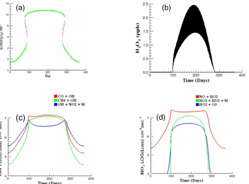
sults (b), the time-dependent variation of noon values of OH loss due to reaction with CO and CH₄and with NO₂throughout the year (c), and the HO₂loss due to reactions with NO and O₃along with the H₂O₂production rate (d). The NO source value in these calculations is the lowest considered and results in a NO_xbackground that ranges from about 40 to 80 ppt. A regional characterization based on this range would be remote

15

tropical forest (National Research Council, 1992). This, and similar NRC characteriza-tions noted later, refers only to NO_x levels and not to other aspects of the chemistry. Smaller NO_x sources would result in an annual low-NO_x cycle characteristic of the re-mote marine troposphere. Both steady-state and time-dependent H₂O₂ mixing ratios vary from a winter low of about 25 ppb to a summer high of about 2 ppb. The annual

20

cycle of H₂O₂ shown in Fig. 2b is qualitatively similar to the observations of Ayers et al. (1996), but with a higher summer maximum as would be expected for higher [NO_x] mixing ratio. Figure 2c indicates that low NO_x conditions prevail throughout the year in this model since nitric acid formation is never competitive with hydrocarbon oxida-tion. A similar comparison of HO₂loss rates (d) shows that the chemistry results in net

25

ozone destruction throughout most of the year. In this model ozone photolysis removes odd oxygen and peroxide formation removes odd hydrogen.

The effect of increasing S_NO from that used in this model is to depress the winter mixing ratio and increase the summer high. The chemistry remains low-NO_x

(15)

through-ACPD

Full Screen / Esc

out the year until, at S_NO≈3.7×105cm−3s−1, a narrow region of bistability first appears that spans a single day, 8 February in late winter and 25 November in fall. Further increases in S_NOincrease the bistable ranges and move their locations towards spring and early fall.

Figure 3 shows the same series of calculations as Fig. 2 with an NO source of

5

2×106cm−3s−1. This S_NO value was chosen because it is in a range characteristic of the northeastern US and is similar to values used by Kleinman (1991) and Jacob et al. (1995). The range of background NO_xmixing ratios in this calculation is 0.5 to 5 ppb, which may be classified as a rural environment (National Research Council, 1992). In this figure and those following the H₂O₂units in the steady-state calculation, part (a),

10

will be shown as Log₁₀ concentration rather than mixing ratio, as in Fig. 2a, to show the full range of summer to winter variation. Mixing ratios will be retained for the time-dependent profile, Fig. 3b, since this will better exhibit the transitions of interest. The H₂O₂ detection limit depends on measurement method, but is of the order of several to several tens of ppt (Lee et al., 2000). Mixing ratios along the abscissa in Fig. 3b and

15

subsequent figures may be regarded as unobservable.

The steady-state profile, Fig. 3a, now exhibits a mushroom shape (Grey and Scott, 1990). In this model the mushroom results from the symmetry of the spring/fall calcula-tion and consists of two conjoined hysteresis curves. The bistable regions extend from days 78 to 91 in the spring (19 March to 1 April and days 275 to 288 in the fall (2–15

20

October). The stable high-NO_x(winter) and low-NO_x (summer) regions are separated by sequences of unstable states shown in red. The instability in the steady-state mode corresponds relatively well to the times at which the dominant pathway for OH reaction, Fig. 3c, switches from nitric acid formation to hydrocarbon oxidation in the spring (day 80, 21 March) and back to nitric acid formation in the fall (day 290, 17 October). The

25

spring increase in time-dependent mixing ratio, Fig. 3b, is most rapid between days 78 and 86 (19–27 March) in reasonable agreement with the switch from high to low-NO_x conditions indicated by the steady-state model (Fig. 3a) and the comparison of OH reaction rates (Fig. 3c). During this time the peroxide mixing ratio increases from

(16)

ACPD

Full Screen / Esc

about 1 ppt to 300 ppt. Thereafter a slower increase to the summer maximum of about 2.5 ppb takes place. In the fall, the most rapid decrease in peroxide mixing ratio occurs between days 280 and 310 (2 October to 6 November) and is roughly the opposite of the spring increase, but over a longer time span. HO₂ loss rates shown in Fig. 3d indicate that the summer low-NO_x regime is ozone producing throughout. It also

indi-5

cates, in contrast with the model in Fig. 2, that significant H₂O₂production occurs only in summer.

As S_NOis increased from the value used in Fig. 3, the bistable regions in the steady-state calculation lengthen and the neck of the mushroom is pinched inward.

The changes resulting from further increase in S_NO are seen in Fig. 4a where the

10

spring and fall bistable regions extend from days 95 to 158 (5 April to 7 June) and 205 to 268 (24 July to 25 September). The NO source used in the model shown in Fig. 4 is S_NO=3.73×106. This value is chosen for display since it is the highest S_NOconsidered for which the time-dependent model shows high to low-NO_x transitions.

It is a consequence of the model design that the steady-state profile is

symmet-15

ric about mid-summer. However, the steady-state calculation suggests that its time-dependent analogue will not be. As days progress through the seasons, a transition from winter to summer conditions will not be forced until 7 June and the corresponding return to winter not forced until 25 September. We thus expect a shift of the time-dependent profile towards the fall side of summer, the shift being greater the more

20

pronounced the pinch in the neck of the mushroom. This is apparent in Fig. 4b along with a much more dramatic asymmetry in the rates of the spring increase and fall de-crease of [H₂O₂]. The high to low-NO_x transition in the time-dependent H₂O₂ profile begins on day 195 (14 July) and is completed in 3 days. The mixing ratio increase in this period is from 0.5 ppt to 1.7 ppb. The much less abrupt fall transition occurs

25

between days 250 and 280 (7 September to 7 October). The mixing ratio decreases from 0.4 ppb to 0.002 ppt during this 30 day interval. The switch between nitric acid formation and hydrocarbon (CO and CH₄) oxidation by OH occurs on days 195 and 248 (Fig. 4c) corresponding to the transitions described for the H₂O₂mixing ratio. The

(17)

ACPD

Full Screen / Esc

chemistry, as expected, is ozone producing throughout the short low-NO_x portion of summer (Fig. 4d). The NO_xrange in this model is about 70 ppb (winter/spring) to 2 ppb (summer), characteristic of rural to urban-suburban regions (National Research Coun-cil, 1992). The correspondence between steady-state and time-dependent models in the time of the spring transition is not as close as that shown in Fig. 3. Although,

ac-5

cording to the steady-state model, a transition should be forced by 7 June it does not occur in the time-dependent case until 14 July.

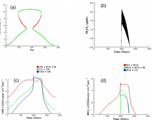
Figure 5 shows the model calculations for S_NO=4.0×106cm−3s−1and a correspond-ing summer to winter [NO_x] of 75 to 130 ppb. This is the next higher source value from that considered in Fig. 4. The mushroom configuration seen in Figs. 3a and 4a has

10

now become a continuous branch of high NO_xstates (Fig. 5a) that persists throughout the year and an isolated branch consisting of low-NO_x summer values and unstable states. An isolated branch of solutions as shown in Fig. 5a is called an “isola” (Grey and Scott, 1990).

For this and higher NO source and [NO_x] background values, the summer low-NO_x

15

states are inaccessible from the time-dependent model. This model remains in a high-NO_xstate throughout the year as indicated by the low H₂O₂mixing ratios (Fig. 5b) and the dominance of nitric acid formation over hydrocarbon oxidation (Fig. 5c). The units in Fig. 5b are parts per quadrillion (ppqd). The HO₂ ozone Production/Loss switch remains in the production position (Figs. 5d and 1), but this is irrelevant since

oxi-20

dant production has been effectively cut off by the switch from low to high-NO_x chem-istry (Fig. 1, OH box). Figure 5d shows the negligible peroxide production rate. As S_NO increases further, the isola shown in Fig. 5a shrinks and finally disappears at S_NO≈1.5×107cm−3s−1.

The NO_xmixing ratios in this model are characteristic of the urban troposphere

(Na-25

tional Research Council, 1992), but the overall model chemistry is not since no signif-icant NMHC are included. In a more comprehensive chemical model, NMHC would result in greater HO_x production and defer an annually dominant high-NO_x regime to higher background NO_x levels. For example, the model study of Honor ´e et al. (2000)

(18)

ACPD

Full Screen / Esc

contains a more realistic urban chemistry. These authors employ a chemistry-transport box model and, for stagnant conditions, find two distinct diurnal equilibria for NO_x emis-sions ∼ a few times 107cm−3s−1 (this estimate is based on their reported maximum NO_xemissions, NO_xemission weight and their maximum mixed layer height of 1.5 km). Their bistable regime occurs at NO_x source values that would result in only high-NO_x

5

solutions in the current model. This effect is also seen in many other models of urban photochemistry in which contour plots of O₃ (or O₃ production) as a function of NO_x and VOC (volatile organic compounds) mixing ratios show the low-NO_x(or NO_x -sensitive or NO_x-limited) to high-NO_x(or VOC-sensitive or VOC-limited) transition mov-ing to higher NO_xvalues as VOC increases. Examples may be found in Sillman (1999)

10

and Tonnesen (1999).

The progression of steady-state solutions shown in Figs. 2a–5a are slices through a three-dimensional (Day, S_NO, [H₂O₂]) surface for selected (Day, [H₂O₂]) planes per-pendicular to the NO source axis. The full set of solutions is shown by the bifurcation surface in Fig. 6. In this figure the Day axis ranges from days 0 through 400 increasing

15

away from the vertex. The NO source axis, labeled Log(S/cm3*s ), ranges from 8 to 4 decreasing away from the vertex and the Log(H₂O₂/cm3) concentrations range through twelve orders of magnitude. The top part of this figure, furthest from the day axis, represents the purely low-NO_x solutions corresponding to situations like that shown in Fig. 2a. Since the annual range of low-NO_x peroxide values is only about 2 ppb,

20

this portion of Fig. 6 has a flat appearance. Slices taken with a plane parallel to the plane defined by the (Day,Log(H₂O₂)) axes generate the profiles in Figs. 2a through 5a. The rightmost such plane generates the purely low-NO_x profile of Fig. 2a. As this plane is moved towards the front of the figure, the pure low-NO_xsolutions give way to mushrooms with increasingly pinched necks, then to a combination of high-NO_x

solu-25

tion branches and low-NO_x isolas and finally to a single branch of high-NO_xsolutions. These last are along the lower part of the figure nearest the day axis.

As stated in the preceding text, to test the robustness of the results some runs have been made with changes in selected parameter values and model reactions.

(19)

Interest-ACPD

Full Screen / Esc

ing variants on the above model are provided by cases in which, as S_NOis increased from low values, a high-NO_x isola, lying under the branch of low-NO_x states, first de-velops in winter. This isola grows and merges with the low-NO_xstates to form a single mushroom branch, similar to Figs. 3a and 4a. The neck of the mushroom then pinches off to leave a continuous branch of high-NO_xstates and a low-NO_xsummer isola as in

5

Fig. 5a. An example of such a system is a model consisting only of reactions (R1)–(R7) supplemented by HNO₃deposition and H₂O₂deposition, photolysis and reaction with OH. The results regarding the correspondence between steady-state bifurcations and time-dependent transitions in the model remain unaltered.

3.2. Annual variation of selected species

10

Table 3 shows the approximate winter to summer change in noon mixing ratio for se-lected species in the time-dependent models shown in Figs. 2b–5b. The corresponding labels in the table are F2–F5. These models are characterized by increasing assumed NO source values and hence by increasing NO_xmixing ratios.

Model F2 is typical of a low-NO_x, ozone destruction environment. Ozone in this case

15

is higher in winter than summer since the enhanced summer photolysis acts to destroy it. This type of annual ozone cycle is seen in the remote marine troposphere at Cape Grim (Ayers et al., 1996). In this environment the seasonal variation of O₃is negatively correlated with H₂O₂and positively correlated with CO.

4. Discussion and summary

20

A series of steady-state and time-dependent models has been run with the objective of determining whether seasonal changes in H₂O₂ mixing ratios are indicative of an underlying instability in the photochemical system.

The annual progression of steady-state values shown in Figs. 2a–5a, begins with an annual cycle that is entirely low-NO_x (Fig. 2a). The time-dependent analogue, Fig. 2b,

(20)

ACPD

Full Screen / Esc

shows a similar variation. This model, with a winter to summer NO_x range of 80 to 40 ppt, is characteristic of the relatively clean remote troposphere (National Research Council, 1992). The annual H₂O₂ mixing ratio is qualitatively similar to the monthly-averaged Cape Grim observations (Ayers et al., 1996), but with somewhat higher sum-mer values.

5

As the assumed NO source is increased the annual progression of steady-states evolves from a purely low-NO_xcycle to one having winter high-NO_x and summer low-NO_x solutions separated by spring and fall transition regions. A region of bistability that contains a run of unstable solutions characterizes the transitions. The branch of solutions shown in Figs. 3a and 4a is known as a mushroom (Grey and Scott, 1990).

10

As S_NOincreases, the neck of the mushroom narrows and finally pinches off to leave a continuous branch of stable high-NO_x states that persists throughout the year and an isolated branch of summer low-NO_x states consisting of stable and unstable solutions (Fig. 5a). As S_NO is increased from the value used in the model shown in Fig. 5, the isola shrinks and ultimately disappears leaving only an annual progression of high-NO_x

15

states. These are shown by the left-most profiles, parallel to the day axis, in Fig. 6. The time-dependent analogues of the steady states, Figs. 2b–5b, do not precisely reflect the transitions in the latter, but there are many qualitative similarities. The most interesting feature of the time-dependent solutions is the asymmetry in spring and fall transitions. This is noticeable in Fig. 3b and obvious in Fig. 4b. The difference in rapidity

20

of spring and fall transitions is a consequence of the different mechanisms involved in H₂O₂production (spring) and loss (fall) mechanisms. In spring, peroxide production is limited by the rapid radical reactions in the chain propagation phase, reactions (R3)– (R5) in Sect. 2.1. In the fall its loss is limited by photolysis and reaction with the OH radical. These loss reactions are included in the model, but are not part of the simplified

25

scheme given by reactions (R1) to (R7).

With reference to Fig. 1 and the simplified reaction set (R1)–(R7), as the NO_x back-ground increases a point is reached at which the O₃ P/L “switch” in the HO₂ box is thrown from ozone loss to production. The autocatalysis indicated by reaction (R8)

(21)

ACPD

Full Screen / Esc

then results in an explosive growth of O₃, OH and HO_2. The rapid increase of H₂O₂ follows suit. In the model shown in Fig. 3b the H₂O₂ production rate resulting from reaction R7 increases from about .1 to .7 ppb/day in the 8-day interval of most rapid H₂O₂growth from 19–27 March. In the model shown in Fig. 4b the corresponding pro-duction rate increases from .007 to 22 ppb/day over the three-day interval from 14–17

5

July. The corresponding fall losses occur between 2 October and 6 November (Fig. 3b) and 7 September to 7 October (Fig. 4b). Loss rates in the former case decrease from .56 to .004 ppb/day and from 1.4 to 3.5×10−6ppb/day in the latter.

5. Conclusions

This paper has explored the relationship between the chemical instability seen in

10

steady-state tropospheric models and corresponding time-dependent behavior. The objective has been to see whether the observed changes in H₂O₂concentrations from summer to winter may, under some circumstances, be interpreted as a manifestation of chemical instability. The rapid growth of [H₂O₂] predicted for spring high to low-NO_xtransitions would be a more definitive indicator of instability than would the slower

15

[H₂O₂] decay in the fall low to high-NO_xtransition. For NO source values greater than 2×106cm−3s−1, the spring transition in the model reported here results in [H₂O₂] in-creases from <10 ppt (i.e. unobservable) to a few hundred ppt in periods of 3 to 7 days. Shorter transition times correspond to higher S_NO, and thus higher background NO_x values. Ideally, observations would be carried out about the spring equinox in a region

20

in which winter [NO_x] is sufficient to govern a high-NO_x regime. A persistent interval, days to weeks, of below detection limit peroxide concentrations followed by a change over an interval of a week or less to a period of detectable and rapidly increasing con-centrations would suggest that bifurcations in the chemistry might be invoked as an explanation. On the other hand, a relatively smooth transition lasting a month would

25

indicate that such a nonlinear effect does not occur.

(22)

ACPD

Full Screen / Esc

concise and readily interpretable. Nature is not so accommodating. Clouds and fogs form and dissipate, rain falls and winds blow. All such events influence the concen-tration of a moderately long-lived and soluble species such as H₂O₂. The result is a degree of variability that is sure to complicate any attempt to relate observations to the consequences of chemical influences. The H₂O₂observations during TOPSE (Snow et

5

al., 2003) illustrate potential problems. The greatest difficulty in carrying out a program of H₂O₂ observations would probably be separating the effects of transport from local photochemistry. Should such a difficulty prove insurmountable it might still be possible to look for evidence of chemical instability in the transitions of a shorter-lived species, such as OH, that would quickly relax to the local chemistry following transport events.

10

Chemical instability is a mathematical characteristic of photochemical models. Due to the magnitude of the changes induced by such instability the question of the exis-tence of atmospheric consequences should be pursued.

References

Atkinson, R., Baulch, D. L., Hampson , R. F. Jr., Kerr, J. A., and Troe, J.: Evaluated kinetic

15

and photochemical data for atmospheric chemistry, J. Phys. Chem. Ref. Data 21, suppl. IV, 1125–1568, 1992.

Ayers, G. P., Penkett, S. A., Gillett, R. W., Bandy, B., Galbally, I. E., Meyer, C. P., Ellsworth, C. M., Bentley, S. T., and Forgan, B. W.: The annual cycle of peroxides and ozone in marine air at Cape Grim, Tasmania, J. Atmos. Chem., 23, 221–252, 1996.

20

Barker, J. R.: A Brief Introduction to Atmospheric Chemistry, in Progress and Problems, in Atmospheric Chemistry, edited by Barker, J. R., World Scientific, Singapore, 1–33, 1995. Bottenheim, J. W. and Shepherd, M. F.: C₂–C₆Hydrocarbon measurements at four rural

loca-tions across Canada, Atmos. Environ., 29, 647–664, 1995.

Crutzen, P. J. and Zimmermann, P. H.: The changing photochemistry of the troposphere, Tellus,

25

43AB, 136–151, 1991.

(23)

ACPD

Full Screen / Esc

Ravishankara, A. R., Kolb, C. E., and Molina, M. J.: Chemical kinetics and photochemical data for use in stratospheric modeling, JPL publication 97-4, 1997.

Dimitroulopoulou, C. and Marsh, A. R. W.: Modelling studies of NO3nighttime chemistry and

its effects on subsequent ozone formation, Atmos. Environ., 31, 3041–3057, 1997.

Field, R. J., Hess, P. G., Kalachev, L. V., and Madronich, S.: Characterization of oscillation and

5

a period-doubling transition to chaos reflecting dynamic instability in a simplified model of tropospheric chemistry, J. Geophys. Res., 102D, 7553–7565, 2001.

Fox, J. L., Wofsy, S. C., McElroy, M. B., and Prather, M. J.: A Stratospheric Chemical Instability, J. Geophys. Res., 87, 11 126–11 132, 1982.

Gnauk, T., Rolle, W., and Spindler, G.: Diurnal variations of atmospheric hydrogen peroxide

10

concentrations in Saxony (Germany), J. Atmos. Chem., 27, 79–103, 1997.

Grey, P. and Scott, S. K.: Chemical Oscillations and Instabilities: Non-linear Chemical Kinetics, Oxford Science Publications, New York, 1990.

Hameed, S., Pinto, J. P., and Stewart, R. W.: Sensitivity of the Predicted CO-OH-CH₄ Pertur-bation to Tropospheric NO_xConcentrations, J. Geophys. Res., 84, 763–768, 1979.

15

Hauglustaine, D. A., Granier, C. Brasseur, G. P., and Megie, G.: The importance of atmospheric chemistry in the calculation of radiative forcing on the climate system, J. Geophys. Res., 99, 1173–1186, 1994.

Hindmarsh, A. C.: Odepack, a systematized collection of ode solvers, in Scientific Computing, edited by Stepleman, R. S. et al., 55–64, North-Holland, Amsterdam, 1983.

20

Holton, J. R. and Lelieveld, J.: Stratosphere-Troposphere Exchange and its role in the budget of tropospheric ozone, in Proceedings of the NATO Advanced Research Workshop, Clouds, Chemistry and Climate, edited by Crutzen, P. and Ramanathan, V., Ringberg, Germany, 173–190, 1994.

Honor ´e, C., Vautard, R., and Beekmann, M.: Photochemical regimes in urban atmospheres:

25

The influence of dispersion, Geophys. Res. Lett., 27, 1895–1898, 2000.

Jacob, D. J., Horowitz, L. W., Munger, J. W., Heikes, B. G., Dickerson, R. R., Artz, R. S., and Keene, W. C.: Seasonal transition from NO_x to hydrocarbon-limited conditions for ozone production over the eastern United States in September, J. Geophys. Res., 100, 9315–9325, 1995.

30

Kalachev, L. V. and Field, R. J.: Reduction of a model describing ozone oscillations in the troposphere, J. Atmos. Chem., 39, 65–93, 2001.

(24)

ACPD

Full Screen / Esc

and High NO_xRegimes, J. Geophys. Res., 96, 20 721–20 733, 1991.

Kleinman, L. I.: Low and High NO_xtropospheric photochemistry, J. Geophys. Res., 99, 16 831– 16 838, 1994.

Konovalov, I. B., Feigin, A. M., and Mukhina, A. Y.: Toward understanding of the nonlinear nature of atmospheric photochemistry: Multiple equilibrium states in the high-latitude lower

5

stratosphere photochemical system, J. Geophys. Res., 104, 3669–3689, 1999.

Lee, M., Heikes, B. G., and O’Sullivan, D. W.: Hydrogen peroxide and organic hydroperoxide in the troposphere: a review, Atmos. Environ., 34, 3475–3494, 2000.

Lelieveld, J., Peters, W., Dentener, F. J., and Krol, M. C.: Stability of tropospheric hydroxyl chemistry, J. Geophys Res., 107, D23, doi:10.1029/2002JD002272, 2002.

10

Levy, H.: Normal atmosphere: Large radical and formaldehyde concentrations predicted, Sci-ence 173, 141–143, 1971.

Madronich, S.: Photodissociation in the atmosphere 1. Actinic flux and the effect of ground reflectance and clouds, J. Geophys. Res., 92, 9740–9752, 1987.

National Research Council: Rethinking the ozone problem in urban and regional air pollution,

15

National Academy Press, Washington, D.C., 1992.

Olivier, J. G. J., Bloos, J. P. J., Berdowski, J. J. M., Visschedijk, A. J. H., and Bouwman, A. F.: A 1990 global emission inventory of anthropogenic sources of carbon monoxide on 1◦×1◦ developed in the framework of EDGAR/GEIA, Chemosphere: Global Change Science, 1, 1–17, 1999.

20

Paulson, S. E.: The Tropospheric Oxidation of Organic Compounds: Recent developments in OH, O₃, and NO₃ Reactions with Isoprene and Other Hydrocarbons, in Progress and Problems in Atmospheric Chemistry, edited by Barker, J. R., World Scientific, Singapore, 111–144, 1995.

Poppe, D., Wallasch, M., and Zimmermann, J.: The dependence of the concentration of OH

25

on its precursors under moderately polluted conditions: a model study, J. Atmos. Chem., 16, 61–78, 1993.

Prather, M. J., McElroy, M. B., Wofsy, S. C., and Logan, J. A.: Stratospheric Chemistry: Multiple Solutions, Geophys. Res. Lett., 6, 163–164, 1979.

Prather, M. J.: Lifetimes and eigenstates in atmospheric chemistry, Geophys. Res. Lett., 21,

30

801–804, 1994.

Press, W. H., Teukolsky, S. A. Vetterling, W. T. and Flannery, B. P.: Numerical Recipes in FORTRAN The Art of Scientific Computing, 2nd Ed., Cambridge University Press, United

(25)

ACPD

Full Screen / Esc

Kingdom, 1992.

Sakugawa, H. and Kaplan, I. R.: H₂O₂and O₃in the atmosphere of Los Angeles and its vicinity: factors controlling their formation and their role as oxidants of SO₂, J. Geophys. Res., 94, 12 957–12 973, 1989.

Sander, S. P., Friedl, R. R., Golden, D. M., Kurylo, M. J., Huie, R. E., Orkin, V. L., Moortgat,

5

G. K., Ravishankara, A. R., Kolb, C. E., Molina, M. J., and Finlayson-Pitts, B. J.: Chemical Kinetics and Photochemical Data for Use in Atmospheric Studies, Evaluation Number 14, JPL Publication 02-25, 2003.

Sillman, S.: The relation between ozone, NO_x, and hydrocarbons in urban and polluted rural environments, Atmos. Environ., 33, 1821–1845, 1999.

10

Snow, J. A., Heikes, B. G., Merrill, J. T., Wimmers, A. J., Moody, J. L., and Cantrell, C. A.: Winter-spring evolution and variability of HO_x reservoir species, hydrogen peroxide and methyl hydroperoxide, in the northern middle to high latitudes, J. Geophys. Res., 108, D4, doi:10.1029/2002JD002172, 2003.

Stewart, R. W., Hameed, S., and Pinto, J. P.: Photochemistry of tropospheric ozone, J.

Geo-15

phys. Res., 82, 3134–3140, 1977.

Stewart, R. W., Hameed, S., and Matloff, G.: A model study of the effects of intermittent loss on odd nitrogen concentrations in the lower troposphere, J. Geophys. Res., 88, 10 697–10 707, 1983.

Stewart, R. W.: Multiple steady states in atmospheric chemistry, J. Geophys. Res., 98, 20 601–

20

20 611, 1993.

Stewart, R. W.: Dynamics of the low to high NO_xtransition in a simplified tropospheric photo-chemical model, J. Geophys. Res., 100, 8929–8943, 1995.

Tie, X., Emmons, L., Horowitz, L., Brasseur, G., Ridley, B., Atlas, E., Stround, C., Hess, P., Klonecki, A., Madronich, S., Talbot, R., and Dibb, J.: Effect of sulfate aerosol on tropospheric

25

NO_x and ozone budgets: Model simulations and TOPSE evidence, J. Geophys. Res., 108, D4, 8364, doi:10.1029/2001JD001508, 2003.

Tinsley, M. R. and Field, R. J.: Dynamic instability in tropospheric photochemistry: An excitabil-ity threshold, Geophys. Res. Lett., 28, 4437–4440, 2001.

Tonnesen, G. S.: Effects of uncertainty in the reaction of the hydroxyl radical with nitrogen

30

dioxide on model-simulated ozone control strategies, Atmos. Environ., 33, 1587–1598, 1999. White, W. H. and Dietz, D.: Does the photochemistry of the troposphere admit more than one

(26)

ACPD

Full Screen / Esc

Yang, P. and Brasseur, G.: Dynamics of the oxygen-hydrogen system in the mesosphere 1. Photochemical equilibria and catastrophe, J. Geophys. Res., 99, 20 955–20 965, 1994.

(27)

ACPD

Full Screen / Esc

Table 1. Variable species included in the present model.

No. Species Flux (cm-2_s-1₎ _{Dep. velocity (cm/s)}

1 O3 7 x 1010 0.4 2 OH 3 HO2 4 H2O2 0.50 5 NO variable 0.016 6 NO2 0.10 7 HNO3 4.0 8 CO 1 x 1011_0.03 9 CH3OOH 0.1 10 CH3O2 11 CH2OOH 12 H2CO 0.25 13 CH3OH 14 NO3 0.1 15 N2O5 4.0 16 HNO2 17 HNO4 4.0 18 C2H4 2 x 109 19 C2H4OHO2 20 C2H4OOH 21 CH2O2 22 C2H6 2 x 109 23 C2H5O2 24 CH3CHO 0.25 25 CH3CO3 26 PAN 1966

(28)

ACPD

Full Screen / Esc

Table 2. Reactions used in the current model. The temperature used for rate evaluation is 278 K. This is the temperature at noon on 1 January in the model. Rate numbers in parentheses correspond to the numbers in Sect. 2.1.

No. Name Rate(cm3_s-1₎

R1 (R1+R2) O3 + hv Æ 2OH 2.03D-07 R2 (R5) NO2 + hv Æ NO + O3 6.42D-03 R3 H2O2 + hv Æ OH + OH 3.45D-06 R4 HNO3 + hv Æ OH + NO2 1.97D-07 R5 PAN + hv Æ CH3CO3 + NO2 2.10D-07 R6 OH + HO2 Æ H2O + O2 1.18D-10 R7 H2O2 + OH Æ HO2 + H2O 1.63D-12 R8 OH + O3 Æ HO2 + O2 5.45D-14 R9 (R4b) HO2 + O3 Æ OH + 2O2 1.82D-15 R10 (R4a) NO + HO2 Æ OH + NO2 8.60D-12 R11 NO + O3 Æ NO2 + O2 1.30D-14 R12 (R3) CO + OH Æ CO2 + HO2 2.44D-13 R13 OH + OH + M Æ H2O2 + M 6.15D-12 R14 (R6) OH + NO2 + M Æ HNO3 + M 1.05D-11 R15 (R7) HO2 + HO2 + M Æ H2O2 + O2 + M 5.33D-12 R16 H2CO + hv Æ 2HO2 + CO 1.66D-05 R17 H2CO + hv Æ CO + H2 2.80D-05 R18 CH3OOH + hv Æ CH3O2 + OH 3.10D-06 R19 CH4 + OH Æ CH3O2 + H2O 4.15D-15 R20 CH3O2 + HO2 Æ CH3OOH + O2 6.74D-12 R21 CH3OOH + OH Æ CH3O2 + H2O 5.46D-12 R22 CH3OOH + OH Æ CH2OOH + H2O 2.30D-12 R23 CH2OOH + M Æ H2CO + OH 1.0DD-12 R24 CH3O2 + CH3O2 Æ 2H2CO + 2HO2 1.95D-13 R25 CH3O2 + CH3O2 Æ H2CO + CH3OH + O2 2.92D-13 R26 CH3OH + OH Æ H2O + CH3O2 8.15D-13 R27 NO + CH3O2 Æ NO2 + H2CO + HO2 8.21D-12 R28 H2CO + OH Æ CO + HO2 1.00D-11 R29 NO3 + hv Æ NO2 + O3 1.56D-01 R30 NO3 + hv Æ NO + O2 2.04D-02 R31 N2O5 + hv Æ NO2 + NO3 1.23D-05 R32 HNO3 + OH Æ NO3 + H2O 1.96D-13 R33 NO2 + O3 Æ NO3 + O2 1.80D-17 R34 NO3 + NO2 Æ NO + NO2 + O2 5.39D-16 R35 NO3 + NO Æ 2NO2 2.76D-11 R36 NO3 + NO3 Æ 2NO2 + O2 1.56D-16 1967

(29)

ACPD

Full Screen / Esc

Table 2. Continued.

No. Name Rate(cm3_s-1₎

R37 OH + NO3 Æ HO2 + NO2 2.30D-11 R38 HO2 + NO3 Æ HNO3 + O2 2.05D-12 R39 HO2 + NO3 Æ OH + NO2 + O2 3.55D-12 R40 NO3 + H2CO Æ HNO3 + HO2 + CO 4.32D-16 R41 N2O5 + H2O Æ HNO3 + HNO3 9.85D-22 R42 NO3 + NO2 + M Æ N2O5 + M 1.35D-12 R43 N2O5 Æ NO3 + NO2 3.97D-03 R44 HNO2 + hv Æ OH + NO 2.50D-03 R45 HNO4 + hv Æ HO2 + NO2 2.03D-06 R46 NO2 + HO2 + M Æ HNO4 + M 1.62D-12 R47 OH + NO + M Æ HNO2 + M 7.90D-12 R48 HNO4 Æ HO2 + NO2 8.21D-03 R49 C2H4 + OH + M Æ C2H4OHO2 8.16D-12 R50 C2H4OHO2 + NO Æ C2H4OOH + NO2 2.00D-12 R51 C2H4OOH + M Æ 2H2CO + HO2 1.96D-02 R52 C2H4 + O3 Æ H2CO + CH2O2 5.85D-19 R53 C2H4 + O3 Æ H2CO + HO2 + OH 5.85D-19 R54 CH2O2 + HO2 Æ H2CO + OH 1.00D-11 R55 C2H6 + OH Æ C2H5O2 + H2O 1.86D-13 R56 C2H5O2 + NO Æ NO2 + HO2 + CH3CHO 9.66D-12 R57 CH3CHO + hv Æ CH3O2 + HO2 + CO 2.21D-06 R58 CH3CHO + hv Æ CH3CO3 + HO2 9.71D-07 R59 CH3CHO + OH Æ CH3CO3 + H2O 1.48D-11 R60 CH3CHO + NO3 Æ CH3CO3 + HNO3 1.77D-15 R61 CH3CO3 + NO2 Æ PAN 9.70D-12 R62 PAN Æ CH3CO3 + NO2 2.05D-05 R63 CH3CO3 + HO2 Æ M 1.51D-11 R64 CH3CO3 + CH3CO3 Æ 2CH3O2 1.75D-11 R65 CH3CO3 + NO Æ NO2 + CH3O2 1.93D-11 1968

(30)

ACPD

Full Screen / Esc

Table 3. Average winter (W) and Summer (S) values in selected species mixing ratios (all in ppb). Models F2 through F5 correspond to the calculations shown in Figs. 2–5.

Model F2 F3 F4 F5 Season W S W S W S W S O3 75 55 70 85 20 100 40 40 NOx .08 .04 5 0.5 70 2 130 75 CO 95 70 90 55 130 55 130 125 1969

(31)

ACPD

Full Screen / Esc

Print Version Interactive Discussion © EGU 2004 O3 OH HC HO2 H2O2 R3 R4b R7 R2 NO2 NO R5:hν R4a HNO3 R6

High NOx Low NOx

R1: hν

Split the O atom from NO2 to form O3 here

Transfer an O atom to NO here Start O3 P/L switch End End

High-NOx, Low NOx switch

Grab an O2 here

Fig. 1. Diagram illustrating the effects of the basic reaction set (R1)–(R7). Boxes bounded by thick lines indicate species having physical sources. The differently colored boxes and arrows indicate Low-NO_xozone loss (blue), low-NO_xozone production (blue and brown) and high-NO_x (red) regimes.

(32)

ACPD

Full Screen / Esc

Fig. 2. Steady-state (a) and time-dependent (b), (c), (d) calculations for the lowest S_NO con-sidered. The NO source here is 4×104cm−3s−1 and results in a summer to winter range of background NO_xof 40 to 80 ppt. Low NO_x conditions prevail throughout the year as shown by the dominance of CO (red) and CH₄(green) oxidation over HNO₃formation (blue) in panel (c). Panel (d) indicates that the net chemistry is ozone destroying throughout the year. The color scheme in parts (c) and (d) is based on the integrated loss by a reaction over an annual cycle, not on the reaction name. In some of the following figures the reactions will be represented by different colors.

(33)

ACPD

Full Screen / Esc

(a) (b)

(c) (d)

Fig. 3. Steady-state (a) and time-dependent (b) and (c) calculations for S_NOof 2×106cm−3s−1. The summer to winter NO_x range in this model is 0.5 to 5 ppb. Part (c) shows that HNO₃ formation (blue) dominates CO (red) and CH₄(green) oxidation in winter, while panel (d) shows the HO2switch (Fig. 1) favors ozone production (red) over loss (blue).

(34)

ACPD

Full Screen / Esc

Fig. 4. Similar to Figs. 2 and 3, but with an assumed S_NOof 3.73×106cm−3s−1. The summer to winter range of NO_xis 2 to 70 ppb. Part(c) shows that HNO₃formation (now in red) dominates CO (green) and CH₄ (blue) oxidation except for a brief period of about 52 days in summer. In panel(d) the dominance of HO₂reaction with NO (red) rather than O₃(blue) facilitates ozone production in the low NO_xregime.

(35)

ACPD

Full Screen / Esc

(a) (b)

(c) (d)

Fig. 5. Similar to Figs. 2–5 but for an assumed S_NO=4.0×106cm−3s−1. The summer to winter NO_x range is 75 to 130 ppb. The OH reaction rates in part(c) indicate high-NO_x dominance throughout the year. In this high-NOxregime H2O2production is negligible(d).

(36)

ACPD

Full Screen / Esc

Fig. 6. H₂O₂ bifurcation surface. Selected slices through this surface parallel to the plane defined by the Day, Log(H₂O₂) axes generate the profiles shown in Figs. 2–5.