Open solar flux estimates from near-Earth measurements of the interplanetary magnetic field: comparison of the first two perihelion passes of the Ulysses spacecraft

HAL Id: hal-00317313

https://hal.archives-ouvertes.fr/hal-00317313

Submitted on 2 Apr 2004

HAL is a multi-disciplinary open access

archive for the deposit and dissemination of

sci-entific research documents, whether they are

pub-lished or not. The documents may come from

teaching and research institutions in France or

abroad, or from public or private research centers.

L’archive ouverte pluridisciplinaire HAL, est

destinée au dépôt et à la diffusion de documents

scientifiques de niveau recherche, publiés ou non,

émanant des établissements d’enseignement et de

recherche français ou étrangers, des laboratoires

publics ou privés.

of the interplanetary magnetic field: comparison of the

first two perihelion passes of the Ulysses spacecraft

M. Lockwood, R. B. Forsyth, A. Balogh, D. J. Mccomas

To cite this version:

M. Lockwood, R. B. Forsyth, A. Balogh, D. J. Mccomas. Open solar flux estimates from near-Earth

measurements of the interplanetary magnetic field: comparison of the first two perihelion passes of the

Ulysses spacecraft. Annales Geophysicae, European Geosciences Union, 2004, 22 (4), pp.1395-1405.

�hal-00317313�

SRef-ID: 1432-0576/ag/2004-22-1395 © European Geosciences Union 2004

Annales

Geophysicae

Open solar flux estimates from near-Earth measurements of the

interplanetary magnetic field: comparison of the first two perihelion

passes of the Ulysses spacecraft

M. Lockwood1,2,3, R. B. Forsyth4, A. Balogh4, and D. J. McComas5

1_{Rutherford Appleton Laboratory, Chilton, Didcot, Oxfordshire, OX11 0QX, UK}

2_{Also at Department of Physics and Astronomy, University of Southampton, Southampton, Hampshire, UK} 3_{Also Visiting Honorary Lecturer, Blackett Laboratory, Imperial College of Science and Technology, London, UK} 4_{Blackett Laboratory, Imperial College of Science and Technology, London, SW7 2BZ, UK}

5_{Space Science and Engineering Division, Southwest Research Institute, San Antonio, TX 78228-0510, Texas, USA}

Received: 21 May 2002 – Revised: 10 July 2003 – Accepted: 11 August 2003 – Published: 2 April 2004

Abstract. Results from all phases of the orbits of the Ulysses

spacecraft have shown that the magnitude of the radial com-ponent of the heliospheric field is approximately independent of heliographic latitude. This result allows the use of near-Earth observations to compute the total open flux of the Sun. For example, using satellite observations of the interplane-tary magnetic field, the average open solar flux was shown to have risen by 29% between 1963 and 1987 and using the aa geomagnetic index it was found to have doubled during the 20th century. It is therefore important to assess fully the ac-curacy of the result and to check that it applies to all phases of the solar cycle. The first perihelion pass of the Ulysses space-craft was close to sunspot minimum, and recent data from the second perihelion pass show that the result also holds at so-lar maximum. The high level of correlation between the open flux derived from the various methods strongly supports the Ulysses discovery that the radial field component is indepen-dent of latitude. We show here that the errors introduced into open solar flux estimates by assuming that the heliospheric field’s radial component is independent of latitude are simi-lar for the two passes and are of order 25% for daily values, falling to 5% for averaging timescales of 27 days or greater. We compare here the results of four methods for estimating the open solar flux with results from the first and second pere-helion passes by Ulysses. We find that the errors are lowest (1–5% for averages over the entire perehelion passes lasting near 320 days), for near-Earth methods, based on either inter-planetary magnetic field observations or the aa geomagnetic activity index. The corresponding errors for the Solanki et al. (2000) model are of the order of 9–15% and for the PFSS method, based on solar magnetograms, are of the order of 13–47%. The model of Solanki et al. is based on the conti-nuity equation of open flux, and uses the sunspot number to quantify the rate of open flux emergence. It predicts that the average open solar flux has been decreasing since 1987, as

Correspondence to: M. Lockwood

(m.lockwood@rl.ac.uk)

is observed in the variation of all the estimates of the open flux. This decline combines with the solar cycle variation to produce an open flux during the second (sunspot maximum) perihelion pass of Ulysses which is only slightly larger than that during the first (sunspot minimum) perihelion pass.

Key words. Interplanetary physics (interplanetary magnetic

fields) – Solar physics, astrophysics and astronomy (mag-netic fields)

1 Introduction

The Ulysses satellite is the first to have sampled the helio-sphere well away from the ecliptic plane. This has allowed a discovery of great importance for solar, heliospheric and solar-terrestrial sciences, namely that the radial component of the heliospheric magnetic field, at a fixed heliocentric dis-tance r, is independent of heliographic latitude 3. To nor-malise the data to a constant heliocentric distance, an r2 de-pendence of radial field is used: this is expected from the increase in flux tube area and is an important part of Parker spiral theory which is very successful in explaining observed heliospheric fields.

The latitudinal uniformity of the radial field Br was first

found to apply as the satellite passed from the ecliptic plane to over the southern solar pole (Smith and Balogh, 1995; Balogh et al., 1995). Subsequently, this result has been con-firmed during the pole-to-pole “fast” latitude scan during the first perihelion pass and during the second ascent of Ulysses to the southern polar region (Lockwood et al. (1999b) and Smith et al. (2001), respectively). Recently, the second peri-helion pass has underlined the generality of the result (Smith et al., 2003; Smith and Balogh, 2003). The first perihelion pass took place during the interval September 1994 until July 1995 when solar activity was low (the average sunspot num-ber during the pass was <R>=23.5). On the other hand, the

second perihelion pass (December 2000 until October 2001) was near sunspot maximum (<R> was 106.5).

Smith and Balogh (1995) noted that the uniformity of the radial field allowed for the computation of the total open solar flux and that it could be explained by excess magnetic pressure at high latitudes close to the Sun. This finding shows that the inner heliosphere is dominated by sheet, and not volume currents. It has been explained further by Suess and Smith (1996) and Suess et al. (1996) in terms of the pressure transverse to the flow in the expanding solar wind at rbetween about 1.5 Rs and 10 Rs, where the plasma beta is

low (the mean solar radius, Rs=6.96×108m): non-radial

so-lar wind flow at r<10 Rsallows for the field to re-distribute,

such that the tangential magnetic pressure is constant, i.e. the radial field is uniform. Because of this result, the radial field seen near Earth Br1can be used to compute the total

flux threading a heliocentric sphere of radius r1=1 AU.

Lockwood (2002) estimated the fraction of the total open solar flux which closes at r between 2.5 Rs and r1 (i.e.

the open flux Fo that does not thread the surface at r=r1)

for solar minimum conditions. Quantitatively, the flux Fo

generates an uncertainty of ±24% in hourly values, falling with an averaging timescale to ±16% in monthly averages and between ±4% in annual values. Thus, the flux threading the surface at r=r1 is a good estimate of that threading

a heliocentric sphere of radius r=2.5 Rs, if the averaging

timescale is sufficiently long. The flux threading r=2.5 Rs

is called the “coronal source flux” or the (unsigned) “open solar flux”, Fs. It is the total flux leaving the solar corona

and entering the heliosphere by threading the hypothetical “coronal source surface”, where the field is purely radial and which is usually taken to be approximately spherical and at r≈2.5 Rs (Wang and Sheeley, 1995; Lockwood et al., 1999;

Lockwood, 2001). If the averaging timescale is large enough for Fo/Fs to be considered negligible, the coronal source

flux estimate can be obtained from:

Fs =4π r12|Br1|/2 + Fo≈4π r12|Br1|/2. (1)

The factor 2 arises because half of the flux through this sur-face is outward (away from the Sun) and half is inward.

Support for the use of Eq. (1), and the approximation in-herent in it, comes from coronal source flux estimates from measurements of the line-of-sight component of the pho-tospheric field (at r=1 Rs). In deriving this line-of-sight

component of the field from magnetograph data, a latitude-dependent “saturation” correction factor must be applied (Wang and Sheeley, 1995). The radial component is then computed by dividing by a cosine factor (so there is no in-formation from over the solar poles). The open flux is then estimated using a method such as the potential field source surface (PFSS) procedure (Schatten et al., 1969), in which the coronal field is assumed to be current-free between the photospheric surface and the coronal source surface, where the field is assumed to be radial. With an improved latitude-dependent saturation correction factor, Wang and Sheeley

(1995) were able to match to the radial field seen at Earth during solar cycles 20 and 21, again using the assumption that Bris independent of latitude in the heliosphere, as found

from the Ulysses observations. Recently, Wang and Sheeley (2002) have shown that this result holds for cycles 22 and 23 as well. Thus, the work of Wang and Sheeley (1995, 2002) gives strong evidence that the Ulysses result on the unifor-mity of the radial heliospheric field is valid throughout cycles 21–23.

The result is important because Eq. (1) allows for the total open flux of the Sun to be computed from near-Earth obser-vations of the Interplanetary Magnetic Field (IMF). Lock-wood et al. (1999) used this to show that the mean open solar flux (averaged over the 11-year solar cycle) had risen by 29% during the interval 1963–1987 for which near-Earth observa-tions of the IMF were available. In addition, these authors developed a procedure to compute the radial component of the near-Earth IMF from the aa geomagnetic index. Appli-cation of Eq. (1) to these data showed that the average open solar flux had increased by a factor of 2.4 during the 20th century.

These studies assumed that the Ulysses result applied at all times, as would be expected from the theory of Suess and Smith (1996) and Suess et al. (1996). In this paper, we study the data from the two perihelion passes of Ulysses in order to analyse the errors introduced by this assumption. We also update the work of Lockwood et al. (1999a, b) to cover data taken after 1995 and thereby place the two perihelion passes in context of the long-term variation of the open solar flux.

2 The Context of the Ulysses perihelion passes

The top panel of Fig. 1 shows the variations of the open solar flux, [Fs]IMF, deduced using Eq. (1) with near-Earth

mea-surements of the radial IMF component, Br1. For

compar-ison, the bottom panel gives the sunspot number, R. The vertical dashed lines mark the intervals of the two Ulysses perihelion passes and the horizontal dashed lines in each panel are the mean values during these intervals.

The first perihelion pass took place between day 280 of 1994 and day 235 of 1995, with the ecliptic plane being crossed on day 73 of 1995. The mean sunspot number for this interval was R=23.5 and the average [Fs]IMF was

4.77×1014Wb. The second perihelion pass took place be-tween day 353 of 2000 and day 301 of 2001, with the eclip-tic plane being crossed on day 144 of 2001. The mean sunspot number for this interval was R=106.5 and the av-erage [Fs]IMFwas 4.85 x 1014Wb.

Thus, the first and second perihelion passes took place un-der very different solar conditions, being near solar minimum and maximum, respectively. However, the open flux derived from near-Earth IMF measurements (and from the Ulysses data themselves, see later) are very similar. In isolation, these data could be interpreted as showing that the open solar flux was almost constant in magnitude. However, the top panel of Fig. 1 shows that, although this is true for solar cycle 20,

1965 1970 1975 1980 1985 1990 1995 2000 2005 0 50 100 150 sunspot number, R Year 3 4 5 6 7 8 [F s]IMF = 2πR1 2_|B r1| [F s ]IMF (10 14 Wb)

Fig. 1. The variation in monthly means of (top) the open solar flux deduced from IMF observations [Fs]IMF=2π r12|Br1|(where

r1=1 AU and Br1is the near-Earth radial component of the IMF) and (bottom) of the sunspot number R. The vertical dashed lines mark the fast latitude scans of the first and second perihelion passes of Ulysses. The horizontal dashed lines in each panel show the mean values during these passes.

there is considerable variation (by a factor of about 2) in the open flux during cycles 21 and 22. Peak open flux occurs roughly two years after peak sunspot number, as found from the PFSS method by Wang et al. (2000b), which has impli-cations for flux tube evolution, as discussed by MacKay et al. (2002) and MacKay and Lockwood (2002).

3 Update of the long-term variation of open solar flux

In this section, we update the results of Lockwood et al. (1999a, b) to cover data taken after 1995. The procedure used is as given by Lockwood et al. (1999a), with the modified im-plementation adopted by Lockwood and Stamper (1999) (i.e. only data from before 1987 were used to derive the procedure for computing Br1from the aa index, leaving data from after

1987 as independent test data). We here refer to the resulting open solar flux estimates as [Fs]aa. Lockwood and Stamper

were able to use data from solar cycle 22 as an independent test of the procedure. The additional data presented here for the rising and maximum phase of cycle 23 thus afford a fur-ther test of the method. In this method, it is important to use 1-year averages to eliminate annual effects, such as the precession of the dipole tilt of the Earth and the obliquity of Earth’s orbit, and seasonal effects, such as the variations in ionospheric conductivity around the magnetometer sites used to generate aa. Thus, Lockwood et al. and Lockwood and Stamper only generated annual means. Here we produce val-ues for one-year intervals, but advance the interval used by one month at a time, so generating a data sequence in which only every 12th data point is fully independent.

1965 1970 1975 1980 1985 1990 1995 2000 2005 3 4 5 6 7 8 F s = 2πR1 2 |B r1| F s from aa Fs (10 14 Wb) Year

Fig. 2. Monthly values of the open solar flux Fs. The

black line shows monthly means deduced from IMF observations

[Fs]IMF=2π r12|Br1|, whereas the red curve shows 1-year values deduced from the aa geomagnetic index [Fs]aa, using the method of Lockwood et al. (1999). The vertical dashed line shows the end of the data interval used by Lockwood et al. in the development of the procedure and the dot-dash line shows the end of the test data presented by these authors. It can be see that the procedure has continued to work well for the additional test data accrued during 1996–2001.

The results for [Fs]aa over 1964–2001 are shown in red

in Fig. 2. For comparison, the black line shows the results from near-Earth IMF data, [Fs]IMF, as presented in Fig. 1.

The vertical dashed line marks the end of the data used in the derivation of the method and the vertical dot-dash line shows the end of the data presented by Lockwood et al. and Lockwood and Stamper. It can be seen that agreement has remained close in the subsequent data.

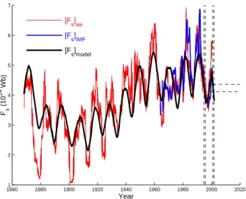
Figure 3 shows the full data sequence of monthly Fs

val-ues from the aa index ([Fs]aain red), extending back to 1868.

The values [Fs]IMF from near-Earth IMF observations are

shown in blue. The black line shows the predictions [Fs]SM

of the model by Solanki et al. (2000). This model is based on a simple continuity equation for open flux (see Eq. (2) be-low), with the emergence rate of new open flux Es, computed

from a semi-empirical function of sunspot number. The loss of open flux is assumed to be linear and Fig. 3 uses the best-fit loss time constant of τ =3.6 years. The model is then integrated forward, from a starting value at the end of the Maunder minimum: the value used is that derived by Lock-wood (2000) from a linear regression between the10Be cos-mogenic isotope abundance in the Dye3 ice sheet core and the [Fs]aa values from the aa index. It can be seen that the

model reproduces the long-term drift and solar cycle varia-tions reasonably well, but cannot reproduce the most rapid variations in the [Fs]aaand [Fs]IMFdata.

The vertical dashed lines show the intervals of the two perihelion passes and the horizontal dashed lines show the open flux values derived from the Ulysses data ([Fs]u, see

Table 1. Estimates of the open solar flux during the first and second perihelion passes of Ulysses.

first second

perihelion fast latitude scan perihelion fast latitude scan open flux, Fs (Fs−[Fs]u)/[Fs]u open flux, Fs (Fs−[Fs]u)/[Fs]u

(1014Wb) (1014Wb)

From Ulysses, (Fs)u 4.54 0 5.05 0

From IMF, [Fs]IMF 4.77 +5% 4.85 −4%

From aa, [Fs]aa 4.31 −5% 5.01 −1%

From PFSS, [Fs]PFSS 3.93 −13% 2.70 −47%

From model, [Fs]SM 4.15 −9% 4.31 −15%

Table 1). It can be seen from Fig. 3 and Table 1 that for both passes the mean open flux seen by Ulysses agrees well (to within 5%) with those derived from the aa index and near-Earth IMF and (to within 15%) with the best-fit model of the open flux variation by Solanki et al. (2000). This model was devised in 1999 to match the open flux variation in the available data, which at that time was for 1868–1996. Thus, the good fit ensures that the model matches well the average open flux seen during the first perihelion pass of Ulysses. Subsequently, the model has matched the evolution of the open flux well and has correctly predicted the open flux seen by Ulysses during its second perihelion pass (see Fig. 3). Thus the model correctly reproduces the fact that the open flux near the peak of cycle 23 is only slightly larger than just before the preceding minimum, as was measured by Ulysses. The Solanki et al. model is not concerned with the dis-tribution of open flux over the solar surface and how this evolves, instead it applies a simple continuity equation to the open flux, assuming a simple linear loss law:

dFS/dt = ES−FS/τ, (2)

where Es is the rate at which new open flux emerges through

the coronal source surface and τ is the loss time constant. Solanki et al. devised a complex function of sunspot number to quantify Es and found a τ of 3.6 years from a best fit to

the data of Lockwood et al.

Figure 4 clarifies the long-term variations by showing 11-year running means. Figure 4a shows the 11-year means of (thin line) the open solar flux <[Fs]aa>11, derived from

the aa index and (thick line) <[Fs]IMF>11 from the

near-Earth IMF observations. Figure 4b shows the 11-year means of the open flux emergence rate <Es>11, deduced from

Eq. (2) using the observed rate of change of Fs and the

best-fit linear loss time constant of τ =3.6 years. Comparison with Fig. 4c shows that the variation of the 11-year mean of the sunspot number <R>11has a somewhat similar form to <Es>11. The plot shows a peak in the average open flux in

1987, after which it has declined. When added to the rise as-sociated with the rising phase of cycle 23, this decline causes the small difference between the solar maximum and solar minimum seen in the comparison of the two Ulysses perihe-lion passes. The downward drift in the open flux after 1987

is caused by a drop in the mean emergence rate associated with a drop in average sunspot numbers.

These variations all assume the Ulysses result, i.e. Eq. (1) applies. We know that use of this equation is, broadly speak-ing, valid because comparisons with the open flux derived from photospheric magnetograms using the PFSS method show that the Ulysses result has applied throughout cycles 20–23 (Wang and Sheeley, 2002). These PFSS data show very similar long-term drifts to those in Fig. 4 (Lockwood, 2003). However, we do not know quantitatively the uncer-tainty incurred in using Eq. (1). In the remainder of this pa-per, we concentrate on quantifying this error using data from the two perihelion passes.

4 Analysis of the first perihelion pass

Figure 5 shows daily means from the first perihelion pass of Ulysses. The top panel shows the radial field, |Bru|, which

varies from negative to positive as Ulysses moves from a large southern polar coronal hole to the corresponding po-lar coronal hole in the Northern Hemisphere, with multiple crossings of current sheet(s) in the streamer belt in-between. Thus, the heliospheric field configuration is very much as expected for sunspot minimum. Figure 5 also gives the he-liocentric coordinates of Ulysses (ru, θu, λu), where ruis the

heliocentric radial co-ordinate of the spacecraft; θuis the

so-lar longitude of the spacecraft (where θu=0 along the

Sun-Earth line) and 3u is the heliographic latitude. The second

panel shows the radial field normalised to r=r1=1 AU using

an r2dependence, |Bru|(ru/r1)2.

Figure 6 compares observations of the heliospheric field |Bru| observed by Ulysses during the first perihelion pass

with those made simultaneously by near-Earth spacecraft |Br1|. In this paper, we use near-Earth interplanetary data

from ACE, which is in a halo orbit around the Lagrange L1 point, and from IMP-8 which is in a 30 RE, near-circular

or-bit around Earth. Thus, both craft are always relatively close to the ecliptic plane and r=r1. Note that data acquisition

from IMP-8 was not continuous at this time and thus, there are gaps in the |Br1|data sequence. The solar wind

18601 1880 1900 1920 1940 1960 1980 2000 2020 2 3 4 5 6 7 [F_s]_aa [F_s]_IMF [F_s]_model Fs (10 14 Wb) Year

Fig. 3. The variation of open solar flux Fs since 1868. The

blue line shows monthly means deduced from IMF observations

[Fs]IMF=2π r12|Br1|, whereas the red curve shows 1-year values

[Fs]aadeduced from the aa geomagnetic index using the method of Lockwood et al. (1999) (see Fig. 2 for a more detailed view of the last 3 cycles). The black curve shows the best fit [Fs]SMusing the open flux continuity model of Solanki et al. (2000). The vertical dashed lines mark the times of the two perihelion passes by Ulysses and the horizontal dashed lines the mean open flux deduced during those passes. Note that the model parameters were obtained from a best fit to data for up to 1986 and thus the values for the two perihe-lion passes are predictions that match the Ulysses observations very well in both cases.

from the radial solar wind speed observed at Ulysses, Vr .

The panels of Fig. 6 show (from top to bottom): (a) the lag L, (b) the radial solar wind speed observed at Ulysses, Vr, (c)

the lagged radial field magnitude, normalised to r=r1=1 AU

using an r2 dependence, |Bru|(ru/r1)2, where |Bru| is the

absolute value of the radial field observed by Ulysses at time tubut plotted here as a function of the time that field passed

through r=r1, i.e. at t1=(tu−L); (d) the radial field

magni-tude observed near the ecliptic plane at r=r1at time t1, |Br1|.

Thin lines show daily means, thick lines are 27-day running means.

The lag L varied between 1 and 3 days, with the largest values at the beginning and end of the pass because then ru

was largest. The variation of ru means that L decreased

towards the centre of the pass but increased again while Ulysses encountered the slow solar wind in the streamer belt. These lags are significant because they are longer than the coherence time of the radial field in the heliosphere. Lock-wood (2002b) has presented the autocorrelation function of the open flux estimated from Eq. (1) (and therefore of the ra-dial field component) and shown that it falls to 0.5 at a lag of 9 h and is only about 0.2 at 1 day and 0.1 at 3 days. Thus it is very important to allow for the lags L, as there is consid-erable variation in the radial field in these intervals.

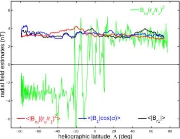
Figure 8 shows the variations of radial field estimates as a function of the heliographic latitude. The green line shows

1880 1900 1920 1940 1960 1980 2000 20 30 40 50 60 70 80 90 <R> 11 Year 4 6 8 10 12 14 <E> 11 (10 13 Wb Yr −1 ) 2 2.5 3 3.5 4 4.5 5 5.5 6 <F s >11 (10 14 Wb)

Fig. 4. Variations of 11-year running means: (top) of the open flux

<[Fs]aa>11 derived from the aa index (thin line) and from near-Earth IMF observations (thick line); (middle panel) of the emer-gence rate <E>11 derived from [Fs]aafrom the aa index with a linear loss rate of open flux with the best-fit time constant of τ =3.6 years; (bottom) of the sunspot number <R>11.

the normalised radial field observed by Ulysses Bru(ru/r1)

2_,

as shown in Fig. 6 and the red line gives 27-day running means time of this absolute values of normalised radial field magnitude, <|Bru|(ru/r1)2>. The black and blue lines give

the 27-day running means of the corresponding radial field magnitude seen near Earth. These near-Earth data are aver-ages over 27-day intervals of time (tu−L), where the Ulysses

observations are made at time tu, and L is the

propaga-tion lag discussed above, and are plotted as the correspond-ing mean of the Ulysses latitude 3u in the 27-day interval

of tu. The black line gives the mean of the observed

ra-dial field magnitude, < |Br1| >. This can be influenced

by transient deflections in the IMF, such as caused by, for example, Coronal Mass Ejections (CMEs), although these effects should largely be cancelled to zero in these 27-day means. The blue line shows an alternative estimate which might be less susceptible to any such effects, made using the magnitude of the B1with the average garden hose angle α, <B1cos(α)>. The value of α used is the average for the

en-tire perihelion pass and is derived from the IMF components observed by IMP-8 and ACE. Although there is some evi-dence that CMEs, Corotating Interaction Regions (CIRs) and current sheet warping, may make B1cos(α) a better estimate

1.4 1.6 1.8 2 2.2 ru (AU) −100 −50 0 50 100 150 200 −50 0 50

days after 1 Jan 1995 Λu (deg) 100 150 200 250 Θu (deg) 0 2 4 6 8 10 12 14 |Bru |(ru /r1 ) 2 (nT) −6 −4 −2 0 2 4 Bru (nT)

Fig. 5. Ulysses data from the first perihelion pass. From top to bot-tom: the radial component of the magnetic field seen by Ulysses

Bruat radial heliocentric distance r=ru; the absolute value of Bru,

normalised to r=r₁=1 AU using an r2dependence, |Bru|(ru/r1)2; the geocentric radial co-ordinate of the spacecraft ru; the solar

lon-gitude of the spacecraft 2u(where 2u=0 along the Sun-Earth line);

and the heliographic latitude of the craft, 3u.

there is little consistent difference on this 27-day averaging timescale and henceforth, the direct that measurement of ra-dial field |Br1|is used. It can be seen that agreement between

the radial field values is good: how good is quantified in the next section.

5 Analysis of errors

In this section, we investigate the deviation of lagged, dis-tance - corrected average radial field seen Ulysses from the radial field seen near Earth:

1Br = {< |Bru(tu)|(ru/r1)2> − < |Br1(tu−L)| >}. (3)

The fractional deviation of the Ulysses radial field from the near-Earth value is then 1Br/|Br1|, the r.m.s. value of

which is εr=<(1Br/|Br1|)2>1/2. Figure 7 is for an

averag-ing timescale T of 27 days: in this section we investigate the use of T between 1 day and 67.5 days (2.5 solar rotations). The dotted line in Fig. 8 shows εr as a function of T . It can

−100 −50 0 50 100 150 200 0 2 4 6 8 10

days after 1 Jan 1995

|Br1 | (nT) 0 2 4 6 8 10 |Bru |(r u /r1 ) 2 (nT) 300 400 500 600 700 800 Vr ( km s − 1 ) 1 1.5 2 2.5 3 lag, L ( days )

Fig. 6. Ulysses and near-Earth IMF data during the first perihelion pass. From top to bottom: the solar wind propagation lag L from (r1, 2u, 3u)to (ru, 2u, 3u); the radial solar wind speed Vr; the

normalised radial field magnitude at r=r1=1 AU, |Bru|(ru/r1)2at time (tu−L), where tuis the observation time at Ulysses; the radial

field magnitude observed near Earth |Br1|. Thin lines show daily means, thick lines are 27-day running means.

be seen that εr is of the order of 50% for T =1 day, but falls

to about 10% for T =27 days, – the averaging interval on which the effects of longitudinal structure and the difference in solar longitude between Earth and Ulysses, 2u(see Fig. 5)

are significant. At greater T , εr converges asymptotically to

7%, the value for averaging over the whole fast latitude scan (which lasts almost twelve 27-day solar rotation periods).

However, this r.m.s. deviation in the radial field εr is not

the same as the error εF in the total open flux estimate FS

incurred by the use of Eq. (1). The total (signed) open flux is half the integral of |B.da| over a whole sphere (where da is a surface area element). For averaging intervals of T this be-comes the sum over N2=(τs/T) solar longitude bins (each

12=2π/N2in extent) and Nλ=(Tp/T) solar latitude bins

(of variable extent 1λ), where τs is the solar rotation period

and Tpis the duration of the pole-to-pole pass.

Fs =(1/2) N2 X j =1 Nλ X i=1 [ru/r1)2|Bru|]ijr1cosλi12r11λi (4)

−80 −60 −40 −20 0 20 40 60 80 −6 −4 −2 0 2 4 6

heliographic latitude, Λ (deg)

radial field estimates (nT)

B ru(ru/r1) 2 <|B r1|> <|B 1|cos(α)> <|B ru|(ru/r1) 2_>

Fig. 7. Ulysses and near-Earth IMF data during the first perihelion pass as a function of the heliographic latitude of Ulysses: (green) the normalised radial field observed by Ulysses |Bru|(ru/r1)2; (red) 27-day means of the normalised radial field magnitude,

<|Bru|(ru/r1)2>; (black) 27-day means of the radial field mag-nitude observed near Earth at time (tuL<|Br1|>; (blue) 27-day means of the radial field magnitude deduced from near Earth mea-surements at time (tuL) from the magnitude of the field B1with the average garden hose angle α, <B1cos(α)>.

Expressing this open flux as a fraction of that deduced from Eq. (1) yields:

Fs/Fs0=(1/4π ) N2 X j =1 Nλ X i=1 [(ru/r1)2|Bru/Br1|]ijcosλi1λi12. (5)

If we average results over any longitudinal structure, be-cause N212=2π , this becomes

Fs/Fs0=(1/2)

Nλ

X

j =1

[(ru/r1)2|Bru/Br1|]ijcos λi1λi. (6)

The fractional error in F_s0, εF , is the error in the ratio

(F_s0/Fs), which is equal to that in its reciprocal. The

uncer-tainty in the sum in Eq. (5) is the square root of the sum of the squares, thus:

εF =(1/2) (_N λ X j =1 εr2cos2λi1λi2 )1/2 . (7)

From Eq. (7) we can compute the effect of the uncertainty εr (given by the dotted line in Fig. 1) in giving the fractional

uncertainty in F_s0, εF. The result, as a function of the

aver-aging timescale T , is the solid line in Fig. 8. Because the near-Earth data is not continuous, it is not possible to com-pute the errors for T less than about 7 days. It can be seen that εF falls to about 5% at T of 27 days and is less than or

equal to this value at all greater T . The solid horizontal line shows the error in F_s0for the whole fast-latitude scan.

0 10 20 30 40 50 60 0 5 10 15 20 25 30 35 40 45 50 % error

averaging interval, T (days)

1994−1995

error in <|B

r1|>

error in <F

s>

Fig. 8. Variations with the averaging timescale, T . (Dashed line) the percentage deviation εr of the normalised radial field magnitude,

<|Bru|(ru/r1)2> at time tu from the value observed near Earth

at time (tu−L), <|Br1|>. (Solid line) the inferred uncertainty εF

in the open solar flux estimate deduced from near-Earth IMF ob-servations [Fs]IMF=2π r12|Br1|. The vertical dashed line marks the mean solar rotation period (in the Earth’s frame) of 27 days. The horizontal dashed line is the value of {<|Bru|(ru/r1)2>−

<|Br1|>}for the full duration of the perihelion pass, the horizontal solid line is the inferred error εFsfor the whole pass.

1.4 1.6 1.8 2 2.2 ru (AU) −50 0 50 100 150 200 250 −50 0 50

days after 1 Jan 2001 Λu (deg) 0 50 100 150 200 Θu (deg) 0 2 4 6 8 10 12 14 |Bru |(ru /r1 ) 2 (nT) −6 −4 −2 0 2 4 Bru (nT)

−500 0 50 100 150 200 250 2 4 6 8 10

days after 1 Jan 2001

|Br1 | (nT) 0 2 4 6 8 10 |B ru |(r u /r1 ) 2 (nT) 300 400 500 600 700 800 Vr ( km s − 1 ) 1 2 3 4 5 lag, L 1u ( days )

Fig. 10. Same as Fig. 6 for the second perihelion pass.

6 Analysis of the second perihelion pass

In this section, we repeat the analysis presented in Sects. 4 and 5 for the second perihelion fast-latitude scan of the Ulysses spacecraft.

Figure 9 shows that the radial field observed by Ulysses is much more structured than during the first pass, in that polar-ity reversals are seen at all latitudes and there are at least 10 clear intervals of both away and toward polarity field. This emphasises the solar maximum nature of the heliospheric field during the second perihelion pass. Note that the so-lar longitude of Ulysses 2u is different from the first pass,

varying between 200◦and 20◦(for the first pass 2u varied

between 270◦and 90◦, see Fig. 5).

Figure 10 shows that the radial solar wind velocity is also more variable than the for the first pass, with several transi-tions between fast to slow solar wind. This introduces more variability into the lag L, superposed on the longer-term vari-ation due to the heliocentric distance ru.

Figure 11 shows the 27-day means of the lagged, range-corrected radial field at Ulysses, as seen by ACE near Earth, as a function of the latitude of Ulysses. As for the first peri-helion pass (see Fig. 7), there is good agreement between the two, and to some extent, the same temporal variations can be seen in the two data sets. Figure 12 shows that the variations of the uncertainties εr and εFwith the averaging timescale T

are very similar indeed to those for the first perihelion pass and that errors are 5% for T ≥ 27 days.

7 Discussion and conclusions

This paper has compared the radial fields observed by Ulysses and by near-Earth spacecraft, with the aim of inves-tigating the use of near-Earth IMF observations to quantify the open solar flux: this test has been applied to the perihe-lion passes of Ulysses for which other factors are minimised. In particular, the ru2 correction factor, allowing for the

ef-fect of the heliocentric distance of Ulysses ru on flux tube

area, varies between about 1.8 and 4.8 during the perihelion passes and so is much closer to unity than for the rest of the Ulysses orbit. In addition, the lower ru(<2.2 AU) near

perihelion means that propagation lags from r=1 AU to the spacecraft are minimised. There is little coherence in the ra-dial field over typical propagation delays L and thus, uncer-tainties in the comparison of simultaneous Ulysses and near-Earth data relating to r=r1would be subject to considerable

errors for larger ru. For ru<2.2 AU, L is less than about 3

days and thus uncertainties in L generally have little effect on averages taken over intervals T of 27 days or longer.

Analysis of the uncertainties introduced by using Eq. (1) shows that they are ≤5% for averaging timescales T ≥27 days. This is true for both the first and second perihelion passes of Ulysses which took place near sunspot minimum and sunspot maximum, respectively. Thus, we can use near-Earth measurements of the radial field and, assuming the Ulysses result that the radial heliospheric field is independent of latitude, derive the total open solar flux to within this un-certainty. The fact that the result applies at sunspot maximum as well as at sunspot minimum, despite the greatly differing natures of the heliospheric field at these times, strongly im-plies that it is a general result, as would be expected from the theoretical explanation by Suess and Smith (1996) and Suess et al. (1996).

The only available test of the application of the Ulysses result on longer timescales comes from the comparisons of the near-Earth radial IMF measurements and the open so-lar fluxes derived from the Potential Field Source Surface (PFSS) method from surface magnetograms (Schatten et al., 1969). Wang and Sheeley (1995, 2002) used such compar-isons to show that the Ulysses result applies over solar cycles 20–23, provided the latitude-dependent line saturation factor is first applied to the photospheric field data. This correction strongly emphasises low-latitude fields, which means that low-order multi-poles dominate the open flux derived. How-ever, there are a number of other assumptions which are used in this method, in addition to the latitude-dependent satura-tion factor. The surface field is assumed to be radial, so that the component normal to the surface can be computed from the observed line-of-sight component (and, even then, no in-formation is available from near the poles). The field is also assumed to be radial at a “coronal source surface” which may only be a hypothetical surface, but which is usually assumed to be spherical, heliocentric and at r=2.5 Rs. The corona

is assumed to be current-free between the photosphere and the coronal source surface (∇×B=0), and Laplace’s equa-tion is solved for Carrington maps of the photospheric field,

−80 −60 −40 −20 0 20 40 60 80 −6 −4 −2 0 2 4 6

heliographic latitude, Λ (deg)

radial field estimates (nT)

B ru(ru/r1) 2 <|B r1|> <|B 1|cos(α)> <|B ru|(ru/r1) 2_>

Fig. 11. Same as Fig. 7 for the second perihelion pass.

assuming that all fields are constant over each Carrington ro-tation interval. Field lines which reach the coronal source surface are defined as open and the flux they constitute quan-tified.

Thus, the conclusion that the Ulysses result can be applied over cycles 20–23, based on a comparison of near-Earth IMF observations and open flux estimates from the PFSS method, is subject to all the above uncertainties introduced by the PFSS method.

Table 1 gives the mean open fluxes for the two perihelion passes derived by a number of methods. The open flux de-rived from the Ulysses data, using Eq. (4), is [Fs]u. The other

values given are all averages over the duration of the perihe-lion passes. The estimates [Fs]IMFand [Fs]aaare derived,

re-spectively, from near-Earth IMF observations and from the aa geomagnetic index (using the procedure of Lockwood et al., 1999a, b) and both make use of Eq. (1). The PFSS procedure, as applied by Wang and Sheeley (2002) yields [Fs]PFSS and

the model of Solanki et al. (1999) gives the values [Fs]SM.

Table 1 also gives the fractional deviation from each of these average open flux estimates from the corresponding value from Ulysses, [Fs]u.

It can be seen from Table 1 that both [Fs]IMF and [Fs]aa

agree with [Fs]uto within the 5% error derived in this paper.

The model predicts values, [Fs]SM, that are slightly low in

both cases, but are still accurate to within 15%. Thus, the model reproduces the fact that the open flux seen during the two Ulysses passes is similar, even though they are at greatly different solar activities.

Table 1 shows that agreement with the PFSS estimates is not so good, [Fs]PFSS being 13% too low for the first pass

and 46% too low for the second pass. As discussed by Wang and Sheeley (2002), photospheric data from the Wilcox So-lar Observatory (WSO) are available up to 1995 but for after that date, data from the Mount Wilson Observatory (MWO)

0 10 20 30 40 50 60 0 5 10 15 20 25 30 35 40 45 50 % error

averaging interval, T (days)

2000−2001

error in <|B

r1|>

error in <F

s>

Fig. 12. Same as Fig. 8 for the second perihelion pass.

were used. The first perihelion pass took place during the in-terval September 1994 until July 1995 and thus, the [Fs]PFSS

value in Table 1 used a mixture of the two data sets. For the second perihelion pass (December 2000 until October 2001), the [Fs]PFSSvalue is based on MWO data alone. Figure 1 of

Wang and Sheeley (2002) shows that [Fs]PFSS was in good

agreement with [Fs]IMFvalue until 1997, but since then it has

been consistently lower. It is this difference that causes the low [Fs]PFSSvalue in Table 2 for the second perihelion pass.

It is not clear if this reflects a feature of the MWO data: how-ever, we note that the same discrepancy [Fs]PFSS<[Fs]IMF

occurred for the WSO data during 1987–1989 in the rising phase of solar cycle 22.

The validity of the Ulysses result, and the low error (<5%) introduced by the use of Eq. (1) allows us to use the near-Earth IMF observations to compute the open flux [Fs]IMF.

The results, shown in Fig. 1, reveal that the open solar flux is not constant, showing a factor of two variations during both cycles 21 and 22. However, thus far, cycle 23, like cycle 20, is showing very little change in open flux.

The longer-term variation in open flux, as derived using the Ulysses result from the aa index, [Fs]aa(Stamper et al.,

1999, Lockwood et al. 1999a, b; Lockwood, 2001, 2002b), agrees well with the predictions of the modelling by Solanki et al. (2000) and Lean et al. (2002). The Solanki et al. model correctly predicts the open flux seen by Ulysses [Fs]u

dur-ing both the perihelion passes (Fig. 3). Thus the model gives us some insight into why the open flux seen in these two passes is so similar (in other words, why cycle 23, like cycle 20 before it, shows only a small variation in the open solar flux). There are a number of contributory factors. First, av-erage sunspot numbers have fallen since 1987 and thus, the flux emergence rate is lower. By Eq. (2), this means that the loss rate has dominated and the average open flux val-ues have fallen. The control of open flux by emergence rate is confirmed by the rise in open flux modelled by Lean et

al. (2002), caused by the rise in sunspot number and emer-gence rate which are the input into their model. In addition, the second Ulysses pass happened to be in a relative min-imum (a “Gnevyshev gap”) in solar activity between two stronger peaks around the maximum of cycle 23: the as-sociated minimum in emergence rate will have made the open flux at the time of the second perehelion pass some-what lower than at other times around this solar maximum. In addition to these effects of reduced emergence rate, cy-cle 22 has also been a somewhat longer solar cycy-cle, allowing more time for the open flux to decay, a relationship predicted by the Solanki et al. (2000) model and noted in observations by Lockwood (2001). Lockwood (2002) has noted that all indicators of open solar flux show a decline since 1987. Su-perposing a solar cycle variation on this longer-term decline in average values has resulted in a peak open flux that is only slightly larger than the value seen during the previous mini-mum. As noted above, Fig. 1 shows that the peak in the open flux was very weak for cycle 20, as it is for cycle 23. This is consistent with the above discussion because cycle 20 was also weaker than the cycle before it, in terms of the sunspot number and thus, the inferred emergence rate (Fig. 4c shows that the 11-year smoothed sunspot number R11 peaked in

1955 and 1987 and Fig. 4b shows that the inferred emergence rate peaked shortly after both R11 maxima). In addition, it

followed an unusually long cycle (number 19).

We conclude that the relative similarity of the open flux values during these two Ulysses passes does not mean that the open flux is constant, rather it is a feature of the general decline in solar activity, average emergence rate and average open solar flux that has been present since 1987. Most so-lar cycles since 1867 are shorter than cycles 19 and 22 (e.g. Lockwood, 2001) and most show higher sunspot numbers and emergence rate (see Fig. 4). From the above, it fol-lows that cycles like 23 and 20, with little open flux variation caused by a downward drift in emergence rate and a long preceding cycle, have been rare in the last 130 years.

Acknowledgements. The authors thank Yi-Ming Wang for

provi-sion of the open flux estimates from the PFSS method. This work was supported by the U.K. Particle Physics and Astronomy Re-search Council. The Editor in Chief thanks N. Ness and another referee for their help in evaluating this paper.

References

Balogh, A., Smith, E. J., Tsurutani, B. T., Southwood, D. J., Forsyth, R. J., and Horbury, T. S.: The heliospheric field over the south polar region of the sun, Science, 268, 1007–1010, 1995. Couzens, D. A. and King, J. H.: Interplanetary medium data book –

supplement 3, national space science data center, Goddard Space Flight Center, Greenbelt, Maryland, USA, 1986.

Hapgood, M. A., Bowe, G., Lockwood, M., Willis, D. M., and Tulunay, Y.: Variability of the interplanetary magnetic field at 1 A.U. over 24 years: 1963–1986, Planet. Space Sci., 39, 411– 423, 1991.

Harvey, K. L. and Zwaan, C.: Properties and emergence of bipolar active regions, Sol. Phys., 148, 85–118, 1993.

Lean, J. L., Wang, Y.-M., and Sheeley Jr., N. R.: The effect of increasing solar activity on the sun’s total and open magnetic flux during multiple cycles: Implications for solar forcing of climate, Geophys. Res. Lett., 29(24), 2224, doi:10.1029/2002GL015880, 2002.

Lockwood, M.: Long-term variations in the magnetic fields of the sun and the heliosphere: their origin, effects and implications, J. Geophys. Res., 106, 16 021–16 038, 2001.

Lockwood, M. and Stamper, R.: Long-term drift of the coronal source magnetic flux and the total solar irradiance, Geophys Res. Lett., 26, 2461–2464, 1999.

Lockwood, M., Stamper, R., and Wild, M. N.: A doubling of the sun’s coronal magnetic field during the last 100 years, Nature, 399, 437–439, 1999a.

Lockwood, M., Stamper, R., Wild, M. N., Balogh, A., and Jones, G.: Our changing sun, Astron. Geophys, 40, 4.10–4.16, 1999b. Lockwood, M.: Relationship between the near-earth interplanetary

field and the coronal source flux: Dependence on timescale, J. Geophys. Res., 107, 1425, doi: 10.1029/2001JA009062, 2002. Lockwood, M.: Twenty-three cycles of changing open

solar magnetic flux, J. Geophys. Res., 108, 1128, doi10.1029/2002JA009431, 2003.

MacKay, D. H. and Lockwood, M.: The evolution of the sun’s open magnetic flux: I. A Single Bipole,. Solar Physics, 207(7), 291– 308, 2002.

MacKay, D. H., Priest, E. R., and Lockwood, M.: The evolution of the sun’s open magnetic flux: II. Full solar cycle simulations, Solar Physics, 209(2), 287–309, 2002.

Schatten, K. H., Wilcox, J. M., and Ness, N. F.: A model of in-terplanetary and coronal magnetic fields, Sol. Phys., 6, 442–455, 1969.

Smith, E. J. and Balogh, A.: Ulysses observations of the radial mag-netic field, Geophys. Res. Lett., 22, 3317–3320, 1995.

Smith, E. J. and Balogh, A.: Open magnetic flux: Variation with latitude and solar cycle, in: Solar Wind Ten: Proceedings of the Tenth International Solar Wind Conference, edited by Velli, M., Bruno, R., and Malara, F., 67–70, 2003.

Smith, E. J., Balogh, A. , Forsyth, R. J., and McComas, D. J.: Ulysses in the south polar cap at solar maximum: Heliospheric Magnetic Geophys. Res. Lett., 28, 4159–4162, 2001.

Smith E. J., Marsden, R. G., Balogh, A., Gl/”ockler, G., Geiss, J., McComas, D. J., McKibben, B., MacDowall, R. J., Lanzerotti, L. J., Krupp, N., Kr¨uger H., and Landgraf, M.: The heliosphere at solar maximum: Ulysses observations, Science, 302, 1165– 1169, 2003.

Solanki , S. K., Sch¨ussler, M., and Fligge, M.: Secular evolution of the sun’s magnetic field since the maunder minimum, Nature, 480, 445–446, 2000.

Solanki , S. K., Sch¨ussler, M. , and Fligge, M.: Secular evolution of the sun’s magnetic flux, Astronomy and Astrophysics, 383, 706–712, 2002.

Stamper, R., Lockwood, M., Wild, M. N., and Clark, T. D. G.: So-lar causes of the long term increase in geomagnetic activity, J. Geophys Res., 104, 28, 325–28, 342, 1999.

Suess, S. T. and Smith, E. J.: Latitudinal dependence of the ra-dial IMF component – coronal imprint, Geophys. Res. Lett., 23, 3267–3270, 1996.

Suess, S. T., Smith, E. J., Phillips, J., Goldstein, B. E ., and Nerney, S.: Latitudinal dependence of the radial IMF component – inter-planetary imprint, Astronomy and Astrophysics, 316, 304–312, 1996.

Ulrich, R. K.: Analysis of magnetic fluxtubes on the solar surface from observations at Mt. Wilson of λ5250 and λ5233, in: Cool Stars, Stellar Systems and the Sun, edited by Giampapa, M. S. and Bookbinder, J. A., Astronom. Soc. of the Pacific, Californian, USA, 265, 1992.

Wang, Y.-M. and Sheeley Jr., N. R.: Solar implications of Ulysses interplanetary field measurements, Astrophys. J., 447, L143– L146, 1995.

Wang, Y.-M. and Sheeley Jr., N. R.: Sunspot activity and the long-term variation of the Sun’s open magnetic flux, J. Geophys. Res., 107, 1425, doi:10.1029/2001JA009062, 2002.

Wang, Y.-M., Sheeley Jr., N. R., and Lean, J.: Understanding the evolution of Sun’s magnetic flux, Geophys. Res. Lett., 27, 621– 624, 2000a.

Wang, Y.-M., Lean, J., and Sheeley Jr., N. R.: The long-term evo-lution of the Sun’s open magnetic flux, Geophys. Res. Lett., 27, 505–508, 2000b.